of different classifiers to sampling density
Eliana Casco Sarmento(1), Elvio Giasson(1), Eliseu Weber(2), Carlos Alberto Flores(3) and Heinrich Hasenack(2)
(1)Universidade Federal do Rio Grande do Sul (UFRGS), Departamento de Solos, Caixa Postal 15100, CEP 91501‑970 Porto Alegre, RS, Brazil.
E‑mail: [email protected], [email protected] (2)UFRGS, Centro de Ecologia, Caixa Postal 15007, CEP 91501‑970 Porto Alegre, RS, Brazil.
E‑mail: [email protected], [email protected] (3)Embrapa Clima Temperado, Caixa Postal 403, CEP 96001‑970 Pelotas, RS, Brazil. E‑mail: [email protected]
Abstract – The objective of this work was to evaluate sampling density on the prediction accuracy of soil orders, with high spatial resolution, in a viticultural zone of Serra Gaúcha, Southern Brazil. A digital elevation model (DEM), a cartographic base, a conventional soil map, and the Idrisi software were used. Seven predictor variables were calculated and read along with soil classes in randomly distributed points, with sampling densities of 0.5, 1,
1.5, 2, and 4 points per hectare. Data were used to train a decision tree (Gini) and three artificial neural networks:
adaptive resonance theory, fuzzy ARTMap; self-organizing map, SOM; and multi-layer perceptron, MLP. Estimated maps were compared with the conventional soil map to calculate omission and commission errors, overall accuracy, and quantity and allocation disagreement. The decision tree was less sensitive to sampling density and had the highest accuracy and consistence. The SOM was the less sensitive and most consistent network. The MLP had a critical minimum and showed high inconsistency, whereas fuzzy ARTMap was more sensitive and less accurate. Results indicate that sampling densities used in conventional soil surveys can serve as a reference to predict soil orders in Serra Gaúcha.
Index terms: appellation of origin, decision tree, digital elevation model, geographic information systems,
neural network, soil mapping.
Predição de ordens de solos com alta resolução espacial: resposta
de diferentes classificadores à densidade de amostragem
Resumo – O objetivo deste trabalho foi avaliar a densidade de amostragem na acurácia de predição de ordens de solos, com alta resolução espacial, em área vitícola da Serra Gaúcha. Para isso, utilizou-se modelo digital de
elevação (MDE) do terreno, base cartográfica, mapa convencional de solos e o programa Idrisi. Sete variáveis
preditoras foram calculadas e lidas junto com as classes de solo, em pontos aleatoriamente distribuídos, nas densidades de 0,5, 1, 1,5, 2 e 4 pontos por hectare. Os dados foram usados para treinar uma árvore de decisão
(Gini) e três redes neurais artificiais: teoria da ressonância adaptativa, fuzzy ARTMap; mapa auto‑organizável,
SOM; e perceptron de múltiplas camadas, MLP. Os mapas estimados foram comparados com o mapa de solos convencional para calcular erros de omissão e de inclusão, exatidão geral, e erros de quantidade e de alocação. A árvore de decisão foi menos sensível à densidade de amostragem e apresentou maior acurácia e consistência. O SOM foi a rede neural com menor sensibilidade e maior consistência. O MLP apresentou mínimo crítico e maior inconsistência, enquanto fuzzy ARTMap apresentou maior sensibilidade e menor acurácia. Os resultados indicam que densidades de amostragem usadas em levantamentos convencionais podem servir de referência para estimar ordens de solos na Serra Gaúcha.
Termos para indexação: denominação de origem, árvore de decisão, modelo digital de elevação, sistemas de informação geográfica, rede neural, mapeamento do solo.
Introduction
Conventional soil surveys have not been able to provide prompt soil information for land-use planning. In the last decades, the lack of information led to the development of modeling techniques to spatially predict soil properties or the occurrence of soil classes in a
reliable way, broadly referred to as digital soil mapping (DSM). According to Lagacherie (2008), DSM can be
defined as the creation and population of spatial soil
Early studies began in the 1970s, but DSM received great impulse in the 1990s, with the spread of technologies such as remote sensing imagery (RS), global positioning system (GPS), geographic information systems (GIS), and advances in computer processing performance. Additionally, the world wide web allowed for the exchange of knowledge between researchers and the creation of online soil information databases, aiming to establish operational DSM systems (McBratney et al., 2003; Sanchez et al., 2009).
In the last two decades, successful researches on the subject have been reported worldwide. These include the application of parametric methods, such as logistic regressions, geostatistical analysis and fuzzy logic, as well as non-parametric approaches, such as machine-learning algorithms (MLA) like decision trees, neural networks, and expert systems (Zhou et al., 2004; Grinand et al., 2008). However, there are no consensus standards or protocols for DSM when compared to conventional soil surveys, which have well-known protocols for almost a century (Hempel et al., 2008).
A critical issue for DSM is the sampling schema, since it is the basis to quantify relationships between the predictor variables and soil properties or soil classes. Zhu (2000), for example, recommends adopting a number of samples equal to 30 times the number of soil classes to be estimated, as the acceptable lower limit. Although there are other studies on sampling density (Zhu, 1997; Shi et al., 2004; Gray et al., 2009), operational recommendations are still scarce, especially
for finer scales. As sampling demands substantial time and costs to do field work and laboratory
analysis, which increase with the used scale, sample size recommendations are needed to evaluate their feasibility and to plan related activities.
Vale dos Vinhedos was the first Brazilian Geografical
Indication for wine, initially established in the category of Indication of Procedence. Currently, the wine sector seeks to raise it to the category of appellation of origin, which requires detailed surveys of the factors that affect vine and wine quality, including soil types and properties. A conventional detailed soil survey was started a few years ago and is still in progress.
Nevertheless, the set of fine‑scale spatial and soil data,
usually not available for most places, provides an excellent basis to evaluate methods for DSM using high spatial resolution data. Moreover, it gives opportunity
to apply DSM techniques to solve real challenges, since two other geographic indications in Serra Gaúcha have already acquired detailed cartographic data and
are also demanding fine‑scale soil maps. It is expected
that knowledge gathered at the Vale dos Vinhedos will help to speed up future detailed soil surveys in Serra Gaúcha.
The objective of this work was to evaluate sampling density on the accuracy prediction of soil orders, with high spatial resolution, using machine-learning algorithms in Serra Gaúcha, Southern Brazil.
Materials and Methods
The experiment was carried out in Vale dos Vinhedos, in the wine production region of Serra Gaúcha, northeast of the state of Rio Grande do Sul, in
Southern Brazil. The climate of the region is classified,
according to Köppen, as Cfb, subtropical with mild summer. The mean temperature of the coldest month is between -3 and 18°C, and the mean temperature of the warmest month is below 22°C, with rainfall evenly distributed throughout the year and total annual rainfall of 1,736 mm (Normal climatológica, 2008). Geology corresponds to the Serra Geral Formation, succession of spills of effusive rocks, mainly basalts and andesites. In general, the relief is complex, showing large variations in elevation, slope, and aspect. Consequently, the distribution of soil types across the landscape shows high spatial variability, with a relative predominance of shallow and stony soils (Flores et al., 1999). The land structure is represented by small farms, based mainly on vine cultivation, with an average area of vineyards per farm of 2.5 hectares.
The study area corresponds to one map sheet of the detailed soil survey (in progress) of Vale dos Vinhedos, and covers 673.5 ha. Geographic coordinates of the bounding box range between 51o34'31.86"W and
51o33'1.86"W, and 29o10'31.78"S and 29o9'1.78"S.
The following materials were used: a 5 m spatial
resolution digital elevation model (DEM) and a stream network, both extracted from an aerophotogrammetric
survey at a scale of 1:10,000, and a detailed soil map
(Sarmento et al., 2008). The soil map was produced through conventional soil survey procedures, including
area contains 155 polygons and 37 individual soil types
belonging to four soil orders: 10 Argissolos (Ultisols), 16
Cambissolos (Inceptisols), 4 Chernossolos (Mollisols), and 7 Neossolos (Entisols). Calculation of predictor variables, spatial analysis, prediction of soil classes, and accuracy assessment were done using the software
Idrisi Taiga GIS (Clark Labs, Worcester, MA, USA). The first step was the selection of prediction variables.
Based on local expert knowledge of soil formation factors and on data availability, variables correlated with variations on moisture regime, erosion and deposition of sediments, organic matter concentration, and depth of the A horizon were considered. Some of the soil formation factors are uniform throughout the study area, including major geology units and climate – particularly high annual rainfall –, whereas others, such as land cover, were not mapped on the spatial resolution used in the present work. However, microclimatic variables and land use are strongly conditioned by
relief. In fact, the strong influence of relief on soil
formation in the evaluated area is well known (Flores et al., 1999), indicating that terrain variables should be good predictors of soil classes (Florinsky et al., 2002). According to Giasson et al. (2011), variables that can
describe these variations in the region are: elevation, slope, aspect, profile curvature, flow accumulation, flow direction, and planar distance from streams. The first six predictors were calculated directly from the
DEM, and the last variable was calculated from the stream network.
Generation of sampling points was done with random
spatial distribution, using five sampling densities,
comprised in the recommended range for detailed soil surveys in Brazil (Manual técnico de pedologia,
2007): 0.5, 1, 1.5, 2, and 4 points per hectare. Since soil classification depends on a number of physical
and chemical characteristics, before sampling, the
conventional soil map was simplified so that the
classes stayed coherent with the selected predictor
variables and could be properly sampled. Soil types
were grouped to the first taxonomic level (order), resulting in a soil map with four classes: Argissolos,
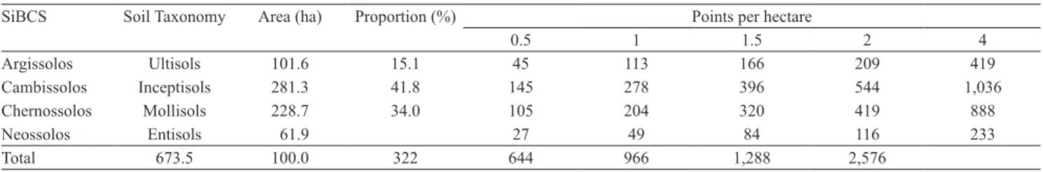
Cambissolos, Chernossolos, and Neossolos. Then, values of predictor variables and soil order, at each sampling point, were collected for all sampling densities. Grouped soil classes and number of sample points per class are shown in Table 1.
Data from sampling points were used to train mLA and to predict the occurrence of soil orders in the whole
study area. Four classification algorithms, based on the concept of mLA, were used: three artificial neural
networks (multi-layer perceptron, MLP; adaptive resonance theory, fuzzy ARTMap; and self-organizing
map, SOM) and a decision tree (Gini). Artificial
neural networks simulate the operation of the structure of neurons and connections of the human brain, whereas decision trees simulate the human process of abstraction through hierarchical categorization (Lippitt et al., 2008). In the training process, 10,000 iterations were used, aiming to optimize the algorithm’s structure and to reach stability on prediction error.
For accuracy assessment, each predicted soil map was compared with the conventional soil map, using all pixels of the study area to calculate error matrices
(Congalton, 1991), and to compute five accuracy indicators: omission errors, expressed as the proportion of a specific class that was estimated as other classes;
commission errors, expressed as the proportion of
different classes included in a specific estimated
class; overall accuracy, expressed as the proportion
of correctly‑classified pixels; quantity disagreement,
which measures the amount of difference between the reference map and the estimated map attributed to the less than perfect match in the proportions of the categories; and allocation disagreement, which measures the amount of difference between the reference map and the estimated map due to the less than optimal match in the spatial allocation of the categories, given
Table 1. Classes of the grouped soil map (order), according to the Brazilian soil classification system (SiBCS) and to Soil Taxonomy, and area, proportion, and number of sample points per class at each sampling density.
SiBCS Soil Taxonomy Area (ha) Proportion (%) Points per hectare
0.5 1 1.5 2 4
Argissolos Ultisols 101.6 15.1 45 113 166 209 419
Cambissolos Inceptisols 281.3 41.8 145 278 396 544 1,036
Chernossolos Mollisols 228.7 34.0 105 204 320 419 888
Neossolos Entisols 61.9 27 49 84 116 233
the proportions of the categories in the reference and estimated map.
Quantity disagreement and allocation disagreement were preferred instead of kappa, which, according to Pontius & Millones (2011), provides redundant information and does not give guidance on how to
improve classification. While kappa measures how
much the agreement is better than random, quantity disagreement and allocation disagreement measure how much the agreement is less than perfect, providing additional information that helps to explain error.
Results and Discussion
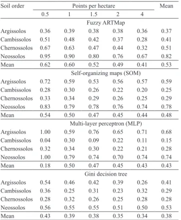
The MLP neural network, with 0.5 point per hectare, simultaneously showed the lowest omission error for Cambissolos and the highest omission error for Neossolos and Argissolos (Table 2). However, it presented minimum commission error for Neossolos and Argissolos (Table 3), since the algorithm could not estimate these classes. In this case, the omission error is
maximized and the commission error is minimized. At the same time, predicted classes that incorrectly receive pixels from unpredicted classes have their omission error reduced and their commission error increased (Congalton, 1991; Pontius & Millones, 2011). The very low omission error observed for Cambissolos indicates that most of the omitted pixels of Neossolos and Argissolos were incorrectly allocated to that class.
Considering only the cases in which all classes could be estimated, the lowest omission errors for Argissolos and Neossolos were found using the Gini decision tree with sampling density of four points per hectare. Lowest errors for Cambissolos and Chernossolos were observed using the MLP neural network, with 1.5 and 4 points per hectare, respectively. The Gini decision tree and MLP neural network also showed the lowest mean omission error per density and overall mean omission error, whereas the neural networks SOM and fuzzy ARTMap had the highest mean omission values for both. Mean omission errors per class varied among the algorithms, with the lowest value
Table 2. Omission errors of estimated soil orders using four
machine learning algorithms and five sampling densities, for
the three neural networks evaluated and for Gini decision tree.
Soil order Points per hectare Mean
0.5 1 1.5 2 4
Fuzzy ARTMap
Argissolos 0.36 0.39 0.38 0.38 0.36 0.37
Cambissolos 0.51 0.48 0.42 0.37 0.28 0.41
Chernossolos 0.67 0.63 0.47 0.44 0.32 0.51
Neossolos 0.95 0.90 0.80 0.76 0.67 0.82
Mean 0.62 0.60 0.52 0.49 0.41 0.53
Self-organizing maps (SOM)
Argissolos 0.72 0.59 0.53 0.56 0.57 0.59
Cambissolos 0.28 0.30 0.26 0.22 0.20 0.25
Chernossolos 0.33 0.34 0.29 0.26 0.25 0.29
Neossolos 0.83 0.79 0.78 0.76 0.74 0.78
Mean 0.54 0.50 0.47 0.45 0.44 0.48
Multi-layer perceptron (MLP)
Argissolos 1.00 0.59 0.76 0.65 0.71 0.68
Cambissolos 0.04 0.30 0.09 0.22 0.11 0.15
Chernossolos 0.32 0.34 0.30 0.22 0.21 0.28
Neossolos 1.00 0.79 0.74 0.70 0.74 0.74
Mean 0.18 0.50 0.47 0.45 0.43 0.43
Gini decision tree
Argissolos 0.54 0.46 0.42 0.39 0.26 0.41
Cambissolos 0.36 0.25 0.31 0.23 0.32 0.29
Chernossolos 0.28 0.32 0.26 0.25 0.28 0.28
Neossolos 0.56 0.55 0.55 0.51 0.50 0.53
Mean 0.43 0.39 0.38 0.35 0.34 0.38
Table 3. Commission errors of estimated soil orders
using four machine learning algorithms and five sampling
densities, for the three neural networks evaluated and for Gini decision tree.
Soil order Points per hectare Mean
0.5 1 1.5 2 4
Fuzzy ARTMap
Argissolos 0.82 0.80 0.76 0.72 0.63 0.75
Cambissolos 0.30 0.29 0.27 0.26 0.23 0.27
Chernossolos 0.30 0.29 0.22 0.23 0.20 0.25
Neossolos 0.73 0.77 0.64 0.59 0.53 0.65
Mean 0.54 0.54 0.47 0.45 0.40 0.48
Self-organizing map (SOM)
Argissolos 0.68 0.68 0.62 0.56 0.54 0.62
Cambissolos 0.37 0.32 0.30 0.30 0.29 0.31
Chernossolos 0.33 0.30 0.28 0.26 0.25 0.28
Neossolos 0.68 0.63 0.55 0.50 0.53 0.58
Mean 0.52 0.48 0.44 0.41 0.40 0.45
Multi-layer perceptron (MLP)
Argissolos 0.00 0.68 0.54 0.57 0.50 0.57
Cambissolos 0.42 0.30 0.35 0.29 0.31 0.33
Chernossolos 0.34 0.22 0.20 0.26 0.19 0.24
Neossolos 0.00 0.51 0.47 0.48 0.33 0.45
Mean 0.38 0.43 0.39 0.40 0.39 0.39
Gini decision tree
Argissolos 0.65 0.56 0.57 0.46 0.57 0.56
Cambissolos 0.28 0.24 0.22 0.22 0.16 0.22
Chernossolos 0.22 0.22 0.23 0.20 0.19 0.21
Neossolos 0.64 0.61 0.60 0.56 0.55 0.59
for Argissolos found by the fuzzy ARTMap neural network; for Cambissolos, by the MLP neural network; for Chernossolos, simultaneously by the MLP neural network and Gini decision tree; and for Neossolos, by the Gini decision tree (Table 2).
Regarding commission errors, except when all classes could not be estimated, the lowest values for Argissolos, Cambissolos, and Chernossolos were found using the Gini decision tree with sampling densities of two, four, and four points per hectare, respectively. For Neossolos, the lowest commission error was obtained using the MLP neural network with four points per hectare. The MLP neural network and Gini decision tree also showed the lowest mean commission errors per density and overall mean commission error, whereas the neural networks SOM and fuzzy ARTMap had the higher mean values for both. Lowest mean commission errors per class for Argissolos, Cambissolos, and Chernossolos were found by the Gini decision tree, and for Neossolos by the MLP neural network (Table 3).
Omission and commission errors tended to decrease as sampling density increased (Tables 2 and 3). The relationship between predictor variables and classes to
be estimated can be better fitted by making decision
rules more consistent and reducing the confusion between classes. As observed by Lippitt et al. (2008), this is particularly important for classes with small extent, which can be subsampled at lower sampling densities.
In almost all cases, Cambissolos and Chernossolos were the classes with the lowest omission and commission errors. This was expected, since these classes were more likely to be correctly mapped as they cover most of the study area, i.e., 41.8 and 34%, respectively. However, this reveals some inadequacy of the random sampling scheme adopted in the present study. According to Pal & Mather (2003), not only the
sample size is important for classification algorithms,
but also the sampling schema. Schmidt et al. (2008) reported that, for small classes, proportional sampling can return better results than a random schema. This may be the case for Neossolos and Argissolos, whose extension corresponds to only 9.1 and 15.1% of the study area, respectively. At lower sampling densities, the number of random samples within classes, with
low occurrence, may not be sufficient to define the
appropriate decision rules (Table 1).
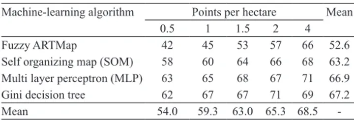
The lowest overall accuracy was found for the neural network fuzzy ARTMap with sampling density of 0.5 point per hectare, while the highest and identical value was obtained for both Gini decision tree with 2 points per hectare and for MLP neural network with 4 points per hectare (Table 4). In fact, the Gini decision tree and MLP neural network performed similarly for all sampling densities, with overall accuracy even above 60% and higher than that for the fuzzy ARTMap and SOM neural networks. However, overall accuracy for the MLP neural network with 0.5 point per hectare is misleading because the algorithm completely omitted two classes. Since the extent of the predicted classes comprises more than 75% of the study area (Table 1), even with the omission of two classes, the percentage of
correctly classified pixels was still high. This indicates
how overall accuracy can lead to misinterpretation of map reliability if it is not analyzed together with other indicators, such as omission and commission errors.
In this sense, quantity disagreement and allocation disagreement provide further information about error, as they decompose the overall disagreement, which
can be defined as 1 minus the overall accuracy, in
two components related to the proportion and to the spatial allocation of the estimated classes, respectively (Pontius & Millones, 2011). In general, the contribution of quantity disagreement (Figure 1 A) for the overall error was smaller than that of the allocation disagreement (Figure 1 B), except for the fuzzy ARTMap neural network. For this algorithm, quantity disagreement was the major component of error and, in most cases, it was clearly above the other algorithms. Furthermore, its steep curve (Figure 1 A) indicates that quantity disagreement is highly sensitive to sampling density.
Among all algorithms, the MLP neural network was the less consistent, showing an unstable,
Table 4. Overall accuracy (%) of estimated maps using four
machine learning algorithms and five sampling densities, for
the three neural networks evaluated and for Gini decision tree.
Machine-learning algorithm Points per hectare Mean
0.5 1 1.5 2 4
Fuzzy ARTMap 42 45 53 57 66 52.6
Self organizing map (SOM) 58 60 64 66 68 63.2
Multi layer perceptron (MLP) 63 65 68 67 71 66.9
Gini decision tree 62 67 67 71 69 67.2
-nonlinear response both in quantity disagreement and in allocation disagreement. As the number of samples increased, an alternation between quantity and allocation was observed. At times, the algorithm did not estimate the correct proportion of classes and, at others, the estimated proportion was correct but many pixels were misallocated. Omission errors (Table 2) and commission errors (Table 3) did not reveal this inconsistence. Overall accuracy (Table 4), instead, suggests a better performance, which shows the importance of considering these two components of error, as proposed by Pontius & Millones (2011),
when evaluating classifiers.
The SOM neural network and Gini decision tree had similar performance, showing the lowest quantity
disagreement among all algorithms. Their flat curves
(Figure 1 A) also indicate a low dependence on the number of samples for this component of error. Allocation disagreement, however, was higher than
that for the fuzzy ARTMap and MLP neural networks, showing a weak response on sampling density (Figure 1 B), with the Gini decision tree presenting lower values. Both the SOM neural network and Gini decision tree were relatively stable in relation to the number of samples and tended to predict classes with the correct proportion, but misallocated some pixels. Visual analysis showed that part of the misallocations occurred close to the boundaries of classes. According to Grimm & Behrens (2010), this is expected because the conventional reference map was drawn by hand,
whereas algorithms used fixed rules to predict classes
on the whole map. As a consequence, some discordance is common near the boundaries, and, in these cases, prediction may be more reliable than the conventional map.
Regarding the magnitude for omission and commission errors and overall accuracy, values were similar to those reported by Coelho & Giasson (2010) for decision trees in predicting soil classes from terrain variables at a coarser spatial resolution. Values found for overall accuracy in the present work were higher than those obtained by Giasson et al. (2011), when predicting soil classes with high spatial resolution from terrain variables using several decision trees. Both studies were developed in similar subtropical
conditions, but used a fixed number of samples. Zhao
et al. (2009) obtained overall accuracy above 80% using neural networks to predict sand, clay, and silt contents with high spatial resolution, whereas the best value found in the present work was 71%, for the MLP neural network and Gini decision tree.
In some aspects, these results partially disagree with Lippitt et al. (2008), who reported better performance for the SOM neural network, when compared to MLP, in classifying remote sensing data. In the present work, MLP showed higher overall accuracy than SOM (Table 4). This may be due to the intrinsic characteristics of the predictor and estimated dataset,
as well as to differences in the configuration of the
neural network structure used. However, SOM was more consistent in terms of quantity disagreement and allocation disagreement (Figure 1) and, therefore, should be preferred (Lippit et al., 2008). This results is in accordance with Srinivasulu & Jain (2006), who recommend that performance evaluation should be done using a wider variety of indicators rather than relying only on a few general statistics, usually employed.
Figure 1. Quantity (A) and allocation disagreement (B) of estimated maps using four machine-learning algorithms and
five sampling densities. ARTMap, fuzzy adaptive resonance
Lippitt et al. (2008) also observed that under optimal sampling, with a high number of samples, different
classifiers usually show low and close error values simultaneously for a specific dataset. In this case,
the number of samples probably is near a limit from which increasing sampling density will not add useful
information and, moreover, can generate overfitting
(Hjort & Marmion, 2008). This may be valid for the Gini decision tree, whose overall accuracy decreased and whose commission errors and quantity disagreement increased at the highest sampling density. The sampling density of four points per hectare matches the upper
limit of the recommended range of field observations
for detailed soils surveys in Brazil (Manual técnico de pedologia, 2007). Therefore, conventional soil survey
sampling schemas may be a helpful guide to drive field
data collection for DSM, at least for detailed scales as used in the present study.
This is relevant when thinking of operational procedures for DSM, since the sampling strategy is a vital issue for the quality of the training data. The more representative samples are introduced
to a classification process, the more accurate and
reliable results will be produced (Kavzoglu, 2009). In the present work, an available soil map was used as reference data, which allowed evaluating the algorithm's performance in response to the number of samples aiming future applications; however, in
practice, most samples must be collected on the field.
The challenge is to obtain a representative sample set large enough so that no relevant information gets lost, but as sparse as possible in order to save labor, time, and costs. In this case, representative means that both size and quality of the sample data are equally important. Therefore, knowledge on the performance,
sensitivity, and reliability of classification algorithms is important to define appropriate sampling (Schmidt
et al., 2008; Kavzoglu, 2009).
In general, the Gini decision tree was less sensitive to sampling density than the three neural networks used, and the fuzzy ARTMap neural network showed the highest sensitivity among all algorithms. For the MLP and SOM neural networks, some indicators were contradictory. Omission and commission errors and overall accuracy indicate that the MLP neural network performed better than SOM, but MLP showed a critical minimum for sampling density below which it could not estimate all classes. However, quantity
disagreement and allocation disagreement indicated that the SOM neural network was the most consistent among all used algorithms, whereas MLP was quite inconsistent. Since the Gini decision tree yields higher accuracies with lower sampling densities, it seems to be the most advantageous choice for predicting occurrence of soil orders, at high spatial resolution, in the study area.
Disregarding differences on algorithm performance, all estimated maps showed more spatial details than the conventional soil map used as a reference, which agrees with previous studies (Zhu, 2000; Hempel et al., 2008). This was expected, since conventional soil maps are restricted to a minimum map delineation size. In Brazil, the minimum mappable area for detailed soil surveys is set to 1.6 ha (Manual técnico de pedologia, 2007). However, in the present
study, the classification algorithms predicted smaller
spatial units, since prediction was done on a pixel with 5 m of spatial resolution. Once a prediction
model is fitted using the selected variables, it is then
uniformly applied to the whole area to be mapped. In conventional surveys, unvisited places must be inferred from soil-landscape relations observed at other locations, which is a less consistent, subjective process. Therefore, in many cases, predicted classes may be more reliable.
Estimated soil classes provide useful information for practical application to viticulture in Serra Gaúcha, Southern Brazil. Given the annual rainfall in the region, soils with good internal drainage, low depth, and low organic matter content are preferred to produce high quality wines. Soil orders allow inferring some soil properties. As vineyards are cultivated in small parcels, decisions need to be made on a compatible spatial resolution basis. It is preferable to have soil orders with good accuracy and consistence than to
have more specific, but less reliable classes. However,
it is necessary to seek other sampling schemes and predictor variables, which may help to improve the
classification of soils in Serra Gaúcha.
Conclusions
2. The Gini decision tree performs better and is less
sensitive to sampling density than the artificial neural
networks, in predicting soil orders at high spatial resolution, in Serra Gaúcha, Southern Brazil.
3. Sampling densities used in conventional soil surveys can serve as a reference to predict soil orders with digital soil mapping at high spatial resolution in Serra Gaúcha.
Acknowledgements
To Conselho Nacional de Desenvolvimento
Científico e Tecnológico and to Financiadora de Estudos e Projetos, for financial support.
References
COELHO, F.F.; GIASSON, E. Comparação de métodos para mapeamento digital de solos com utilização de sistema de informação
geográfica. Ciência Rural, v.40, p.2099-2106, 2010.
CONGALTON, R.G. A review of assessing the accuracy of
classification of remotely sensed data. Remote Sensing of Environment, v.37, p.35-46, 1991.
FLORES, C.A.; FASOLO, P.J.; PÖTTER, R.O. Solos: levantamento semidetalhado. In: FALCADE, I.; MANDELLI, F. (Org.). Vale dos Vinhedos: caracterização geográfica da região. Caxias do Sul:
EDUCS; Bento Gonçalves: Embrapa Uva e Vinho, 1999. p.87‑134. FLORINSKY, I.V.; EILERS, R.G.; MANNING, G.; FULLER, L.G.
Prediction of soil properties by digital terrain modeling.
Environmental Modeling and Software, v.17, p.295-311, 2002.
GIASSON, E.; SARMENTO, E.C.; WEBER, E.; FLORES, C.A.; HASENACK, H. Decision trees analysis for digital soil mapping on subtropical basaltic steeplands. Scientia Agricola, v.68, p.167-174, 2011.
GRAY, J.M.; HUMPHREYS, G.S.; DECKERS, J.A. Relationships
in soil distribution as revealed by a global soil database. Geoderma, v.150, p.309-323, 2009.
GRIMM, R.; BEHRENS, T. Uncertainty analysis of sample
locations within digital soil mapping approaches. Geoderma, v.155, p.154-163, 2010.
GRINAND, C.; ARROUAYS, D.; LAROCHE, B.; MARTIN, M.P. Extrapolating regional soil landscapes from an existing soil map:
sampling intensity, validation procedures, and integration of spatial context. Geoderma, v.143, p.180-190, 2008.
HEMPEL, J.W.; HAMMER, R.D.; MOORE, A.C.; BELL, J.C.; THOMPSON, J.A.; GOLDEN, M.L. Challenges to digital
soil mapping. In: HARTEMINK, A.E.; MCBRATNEY, A.;
MENDONÇA-SANTOS, M. de L. (Ed.). Digital soil mapping with limited data. New York: Springer, 2008. p.81‑90.
HJORT, J.; MARMION, M. Effects of sample size on the accuracy of geomorphological models. Geomorphology, v.102, p.341-350, 2008.
KAVZOGLU, T. Increasing the accuracy of neural network classification using refined training data. Environmental Modelling and Software, v.24, p.850-858, 2009.
LAGACHERIE, P. Digital soil mapping: a state of the art. In.:
HARTEMINK, A.E.; MCBRATNEY, A.; MENDONÇA-SANTOS, M. de L. (Ed.). Digital soil mapping with limited data. New York:
Springer, 2008. p.3-14.
LIPPITT, C.D.; ROGAN, J.; LI, Z.; EASTMAN, J.R.; JONES,
T.G. Mapping selective logging in mixed deciduous forest: a
comparison of machine learning algorithms. Photogrammetric Engineering and Remote Sensing, v.74, p.1201-1211, 2008.
MANUAL técnico de pedologia. 2.ed. Rio de Janeiro: IBGE, 2007.
300p.
MCBRATNEY, A.B.; MENDONÇA-SANTOS, M. de L.; MINASNY, B. On digital soil mapping. Geoderma, v.117, p.3-52, 2003.
NORMAL climatológica: Estação Agroclimática da Embrapa Uva e Vinho, Bento Gonçalves, RS: dados médios do período de 1961 a 1990. Bento Gonçalves: Embrapa Uva e Vinho, 2008. Disponível em: <http://www.cnpuv.embrapa.br/prodserv/meteorologia/ bento‑normais.html>. Acesso em: 05 nov. 2010.
PAL, M.; MATHER, P.M. An assessment of the effectiveness
of decision tree methods for land cover classification. Remote Sensing of Environment, v.86, p.554-565, 2003.
PONTIUS, R.G.; MILLONES, M. Death to Kappa: birth of
quantity disagreement and allocation disagreement for accuracy assessment. International Journal of Remote Sensing, v.32, p.4407-4429, 2011.
SANCHEZ, P.A.; AHAMED, S.; CARRÉ, F.; HARTEMINK, A.E.;
HEMPEL, J.; HUISING, J.; LAGACHERIE, P.; MCBRATNEY,
A.B.; MCKENZIE, N.J.; MENDONÇA-SANTOS, M. de L.; MINASNY, B.; MONTANARELLA, L.; OKOTH, P.; PALM, C.A.;
SACHS, J.D.; SHEPHERD, K.D.; VÅGEN, T.‑G.; VANLAUWE,
B.; WALSH, M.G.; WINOWIECKI, L.A.; ZHANG, G.-L. Digital soil map of the world. Science, v.325, p.680-681, 2009.
SANTOS, H.G. dos; JACOMINE, P.K.T.; ANJOS, L.H.C. dos; OLIVEIRA, V.A. de; OLIVEIRA, J.B. de; COELHO, M.R.;
LUMBRERAS, J.F.; CUNHA, T.J.F. (Ed.). Sistema brasileiro de
classificação de solos. 2.ed. Rio de Janeiro: Embrapa Solos, 2006.
306p.
SARMENTO, E.C.; FLORES, C.A.; WEBER, E.; HASENACK,
H.; POTTER, R.O. Sistema de informação geográfica como apoio
ao levantamento detalhado de solos do Vale dos Vinhedos. Revista Brasileira de Ciência do Solo, v.32, p.2795-2803, 2008.
SCHMIDT, K.; BEHRENS, T.; SCHOLTEN, T. Instance selection
and classification tree analysis for large spatial datasets in digital
soil mapping. Geoderma, v.146, p.138-146, 2008.
SHI, X.; ZHU, A.X.; BURT, J.E.; QI, F.; SIMONSON, D.
A case-based reasoning approach to fuzzy soil mapping. Soil Science Society of America Journal, v.68, p.885-894, 2004.
SRINIVASULU, S.; JAIN, A. A comparative analysis of training methods for artificial neural network rainfall‑runoff models.
ZHAO, Z.; CHOW, T.L.; REES, H.W.; YANG, Q.; XING, Z.;
MENG, F.R. Predict soil texture distributions using an artificial
neural network model. Computers and Electronics in Agriculture, v.6, p.36-48, 2009.
ZHOU, B.; ZHANG, X.‑G.; WANG, R.‑C. Automated soil
resources mapping based on decision tree and Bayesian
predictive modeling. Journal of Zhejiang University Science, v.5, p.782-795, 2004.
ZHU, A.X. A similarity model for representing soil spatial
information. Geoderma, v.77, p.217-242, 1997.
ZHU, A.X. Mapping soil landscape as spatial continua: the neural
network approach. Water Resources Research, v.36, p.663-677, 2000.