www.nonlin-processes-geophys.net/23/269/2016/ doi:10.5194/npg-23-269-2016
© Author(s) 2016. CC Attribution 3.0 License.
Fractal behavior of soil water storage at multiple depths
Wenjun Ji1, Mi Lin1, Asim Biswas1, Bing C. Si2, Henry W. Chau3, and Hamish P. Cresswell4
1Department of Natural Resource Sciences, McGill University, 21111 Lakeshore Road, Ste-Anne-de-Bellevue, Québec, H9X3V9, Canada
2Department of Soil Science, University of Saskatchewan, Saskatoon, Saskatchewan, S7N5A8, Canada
3Department of Soil and Physical Sciences, Lincoln University, P.O. Box 85084, Lincoln, 7647 Christchurch, New Zealand 4CSIRO Land and Water, 2601 Canberra, ACT, Australia
Correspondence to:Asim Biswas ([email protected])
Received: 29 December 2015 – Published in Nonlin. Processes Geophys. Discuss.: 4 February 2016 Revised: 13 June 2016 – Accepted: 14 June 2016 – Published: 15 August 2016
Abstract.Spatiotemporal behavior of soil water is essential to understand the science of hydrodynamics. Data intensive measurement of surface soil water using remote sensing has established that the spatial variability of soil water can be described using the principle of self-similarity (scaling prop-erties) or fractal theory. This information can be used in de-termining land management practices provided the surface scaling properties are kept at deep layers. The current study examined the scaling properties of sub-surface soil water and their relationship to surface soil water, thereby serving as supporting information for plant root and vadose zone mod-els. Soil water storage (SWS) down to 1.4 m depth at seven equal intervals was measured along a transect of 576 m for 5 years in Saskatchewan. The surface SWS showed multi-fractal nature only during the wet period (from snowmelt un-til mid- to late June) indicating the need for multiple scaling indices in transferring soil water variability information over multiple scales. However, with increasing depth, the SWS became monofractal in nature indicating the need for a sin-gle scaling index to upscale/downscale soil water variability information. In contrast, all soil layers during the dry period (from late June to the end of the growing season in early November) were monofractal in nature, probably resulting from the high evapotranspirative demand of the growing veg-etation that surpassed other effects. This strong similarity be-tween the scaling properties at the surface layer and deep layers provides the possibility of inferring about the whole profile soil water dynamics using the scaling properties of the easy-to-measure surface SWS data.
1 Introduction
Knowledge on the spatial distribution of soil water over a range of spatial scales and time has important hydrologic applications including assessment of land–atmosphere in-teractions (Sivapalan, 1992), performance of various engi-neered covers, monitoring soil water balance, and validating various climatic and hydrological models (Rodriguez-Iturbe et al., 1995; Koster et al., 2004). However, high variabil-ity in soil is a major challenge in hydrology (Quinn, 2004) as the distribution of soil water in the landscape is con-trolled by various factors and processes operating at differ-ent intensities over a variety of extdiffer-ents (Entin et al., 2000). The individual and/or combined influence of these physical factors (e.g., topography, soil properties) and environmen-tal processes (e.g., runoff, evapotranspiration, and snowmelt) gives rise to complex and nested effects, which in turn evolve a signature in the spatial organization (Western et al., 1999) or patterns in soil water as a function of spatial scale (Kachanoski and de Jong, 1988; Kim and Barros, 2002; Biswas and Si, 2011a). This complexity makes the manage-ment decision difficult at a scale other than that of measure-ment. Therefore, it is necessary to transfer variability infor-mation from one extent (e.g., pedon) to another (e.g., large catchment), which is called scaling.
270 W. Ji et al.: Fractal behavior of soil water storage at multiple depths
have a typical size or scale, a value around which individual measurements are centered. So the probability of measuring a particular value will vary inversely as a power of that value, which is known as the power-law decay, a typical principle of the scaling process. Now, as the spatial distribution of soil water follows the power-law decay (Hu et al., 1997; Kim and Barros, 2002; Mascaro et al., 2010), the spatial variability can be investigated and characterized quantitatively over a large range of measurement extents using the fractal theory (Mandelbrot, 1982). When the spatial distribution of soil wa-ter is the response of some linear processes, the scaling can be done using a single coefficient over multiple scales and the distribution shows monofractal behavior. However, the spatial distribution of soil water is the nonlinear response of multiple factors and processes acting over a variety of scales and therefore needs multiple scaling indices (multifractals) for quantifying spatial variability (Hu et al., 1997; Kim and Barros, 2002; Mascaro et al., 2010).
The multifractal behavior in the surface soil water as a re-sult of temporal evolution of wetting and drying cycles has been reported from the sub-humid environment of Oklahoma by Kim and Barros (2002). Mascaro et al. (2010) reported the multifractal behavior of soil water, which was ascribed as a signature of the rainfall spatial variability. Though these measurements can provide a quick estimate of soil water over a large area, they are limited to very few centimeters of the soil profile. These studies reported the multifractal behavior of only the surface soil water indicating the superficial scal-ing properties. Surface soil layer is exposed to direct environ-mental forces and is the most dynamic in nature. The scaling properties of surface soil water can be used for land man-agement practices, provided the observed scaling properties remain the same for the deep layers such as vadose zone or the whole soil profile. Understanding the overall hydrologi-cal dynamics in soil profiles requires information on the shydrologi-cal- scal-ing properties and the nature of the spatial variability of soil water over a range of scales at deep layers as well (Biswas et al., 2012c). The information on the similarity in the nature of the spatial variability of soil water between the surface layer and deep layers may also help inferring about the soil pro-file hydrological dynamics. Therefore, the objectives of this study were to examine over time the scaling properties of sub-surface layers and their relationship with surface layers at different initial soil water conditions. We have examined the scaling properties of soil water storage at each layer and their trend with increasing depth from the surface (cumula-tive depth) over a 5-year period from a hummocky landscape from central Canada using the multifractal approach. The re-lationship between the scaling properties of the surface layer and the subsurface layers was also examined using the joint multifractal analysis.
2 Materials and methods
2.1 Study site and data collection
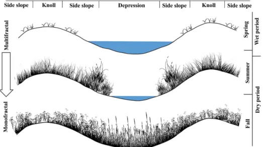
A field experiment was carried out at St. Denis National Wildlife Area (52◦12′N, 106◦50′W;∼549 m mean above sea level), which is located 40 km east of Saskatoon, Saskatchewan, Canada. The landscape of the study area is hummocky with a complex sequence of slopes (10 to 15 %) extending from differently sized rounded depressions to ir-regular complex knolls and knobs, a characteristic landscape of the North American prairie pothole region encompassing approximately 780 000 km2from north-central United States to south-central Canada (National Wetlands Working Group, 1997). Some of these potholes are seasonal in nature meaning to store water in the spring (wet period) and drying out during late summer and in fall season (dry period) (Fig. 1). Variable water distribution within the landscape and in different land-form elements such as side slopes, knolls, and depressions support vegetation differently. For example, the large amount of stored water in depressions provide a luxurious supply of water to growing plants compared to knolls (Fig. 1). A tran-sect of 128 points (576 m long) extending in the north–south direction covering multiple knoll-depression cycles was es-tablished in 2004 at the study site to examine the soil water variation at field scale. The sample points were selected at 4.5 m regular intervals along the transect to catch the system-atic variability of soil water. Soil water measurements were carried out at every 20 cm depth down to 140 cm along the transect over the period of 2007 to 2011, among which the surface soil water (0 to 20 cm) was measured using verti-cally installed time domain reflectometry (TDR) probes and a metallic cable tester (model 1502B, Tektronix, Beaverton, OR), while deeper layers down to 140 cm were measured us-ing a neutron probe (model CPN 501 DR Depthprobe, CPN International Inc., Martinez, CA) (Biswas et al., 2012a). Soil water content data were then multiplied by depth and added together to obtain the overall soil profile water storage so as to examine the fractal behavior of soil water storage (SWS) at different depths over time. A detailed description of the study site, development of the transect, measurement of soil water and the calibration of measurement instruments can be found in earlier publications from this project (e.g., Biswas et al., 2012a).
2.2 Data analysis
Various methods including geostatistics (Grego et al., 2006), spectral analysis (Kachanoski and de Jong, 1988), and wavelet analysis (Biswas and Si, 2011a, b) have been used to examine the scale-dependent spatial patterns of SWS. These methods generally deal with how the second moment of SWS changes with scales or frequencies. When the statistical dis-tribution of SWS is normal, the second moment plus the av-erage provide a complete description of the spatial series.
Figure 1.Conceptual schematics showing the vegetation growth patterns over the landscape at different times of the year. The figure is developed based on field observations and the scale is arbitrary.
However, for other distributions (e.g., left skewed distribu-tion) higher-order moments are necessary for a complete de-scription of the spatial series. For example, let us define the
qth moment of a spatial serieszas zq. In this situation, for a positive value ofq, theqth moment magnifies the effect of larger numbers and diminish the effect of smaller numbers inz. While, on the other hand, for a negative value ofq, the
qth moment magnifies the effect of small numbers and di-minish the effect of large numbers in the spatial seriesz. In this way, using variable moments, we can look at the effect of the magnitude of the data in a series and better characterize its spatial variability.
2.2.1 Statistical self-similarity or scale invariance Soil water is highly variable in space and time. If the variabil-ity in the spatial/temporal distribution remains statistically similar at all studied scales, the SWS is assumed to be self-similar (Evertsz and Mandelbrot, 1992). Self-self-similarity, also called scale invariance, is closely associated with the transfer of information from one scale to another. We used the mul-tifractal analysis to explore self-similarity or inherent differ-ences in scaling properties of SWS in this study.
2.2.2 Multifractal analysis
On the spatial domain of the studied field, multifractal anal-ysis was used to characterize the scaling property of SWS by statistically measuring the mass distribution (Zeleke and Si, 2004). The spatial domain or the data along the tran-sect was successively divided into self-similar segments fol-lowing the rule of the binomial multiplicative cascade (Ev-ertsz and Mandelbrot, 1992). This method required that the two segments divided from a unit interval to be of equal
length. With regards to a unit massM (a normalized prob-ability distribution of a variable or measured in a generalized case) relating to the unit interval, the weight was also parti-tioned into [h×M] and [(1−h)×M], wherehwas a ran-dom variable (0≤h≤1) governed by a probability density function. Sequentially, the new subsets with their associated mass were equally divided into smaller parts. In this way, multifractal analysis was able to describe the scaling prop-erties for the higher-order moments compared to semivari-ogram, which can only measure the scaling properties of the second moment. In a special case, if the scaling properties do not change withq, the spatial series can be identified as monofractal, when one scaling coefficient is enough to char-acterize scaling property of SWS. Generally, the multifractal analysis is good at measuring the highly fluctuated mass (box size) within a scale interval. This also provides physical in-sights at all scales regardless of any ad hoc parameterization or homogeneity assumptions in the analysis (Schertzer and Lovejoy, 1987).
For SWS spatial series, the scale-invariant mass exponent, was termed asτ (q)(Liu and Molz, 1997):
h[1z(x)]qi ∝xτ (q), (1)
where z was the SWS spatial series, x was the lag dis-tance and the symbol∝indicated proportionality. Theτ (q)is widely used in multifractal analysis. If the plot ofτ (q)vs.q
272 W. Ji et al.: Fractal behavior of soil water storage at multiple depths
in mean value of SWS, this model simulated a cascade pro-cess with a scaling function in an empirical moment. It is thus used here to compare and characterize the observed scaling properties with a reference to the monofractal behavior. The goodness-of-fit between theτ (q)curves and the UM model was tested using the chi-square test. The sum of squared residuals (SSRs) between theτ (q)curve and the UM model was also calculated to test the deviation. The τ (q) curves over the range ofq values (in this study−15 to 15 at 0.5 in-tervals) were fitted with a linear regression line (referred to as a single fit). The linear fitting of theτ (q)curves withq <0 andq >0 (referred to as segmented fit) was also completed. The difference between the mean of slopes and segmented fits (for positive and negativeq values) was checked using the Student’sttest.
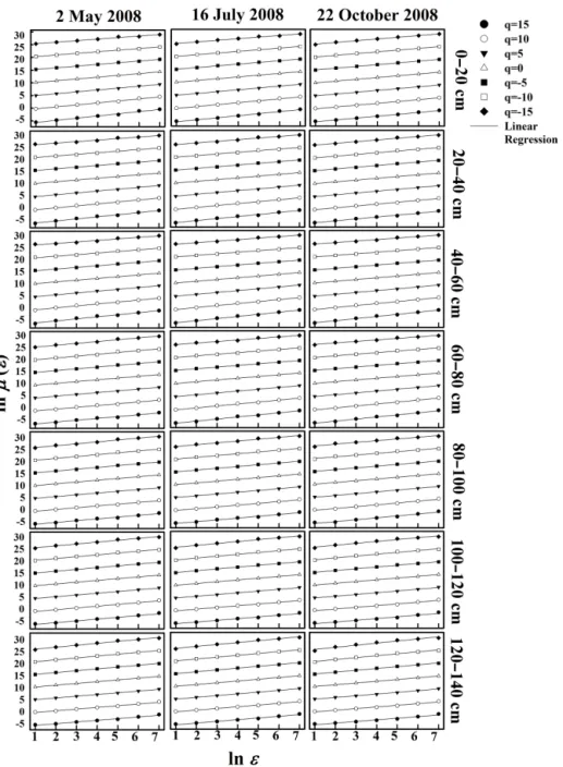
In a similar manner to Eq. (1), the qth-order normalized probability measure of SWS,µ(q,ε)(also known as the par-tition function), is proven to vary with the scale size:
µi(q, ε)=
pi(ε)
q
P
i
pi(ε)
q ∝(ε/L)
τ (q),
(2)
whereεis scale size in theith segment andpi(ε)is the
prob-ability of a measurepi(ε)and measures the concentration of
a variable of interest (e.g., SWS) by dividing the value of the variable in the segment to the whole support length (e.g., to the whole transect of lengthLunits) (Meneveau et al., 1990; Evertsz and Mandelbrot, 1992). The mass exponentτ (q)was related to the probability of mass distribution of SWS.
Moreover, the fractal dimension of the subsets of seg-ments in scale sizeεwas measured by the multifractal
spec-trum f (q). When a coarse Hölder exponent (local scaling
indices) ofαwas at the limit asε→0,f (q)was calculated as follows (Evertsz and Mandelbrot, 1992):
f (q)=lim
ε→0
logε
L
−1X
i
µi(q, ε)logµi(q, ε), (3)
and the local scaling indices,α, were given by
α(q)=lim
ε→0
logε
L
−1X
i
µi(q, ε)logpi(ε). (4)
Noting that f (α) was determined through the Legendre transform of theτ (q)curve:f (α)=qα(q)−τ (q)(Chhabra and Jensen, 1989).
The multifractal spectrum is a powerful tool in portraying the similarity and/or differences between the scaling proper-ties of the measures (e.g., SWS). The width of the spectrum (αmax–αmin) was used to examine the heterogeneity in the local scaling indices. The wider the spectrum, the higher the heterogeneity in the distribution of SWS and vice versa. Sim-ilarly, the height of the spectrum corresponded to the dimen-sion of the scaling indices. The smallf (q)values indicated rare events (extreme values in the distribution), whereas the
largest value was the capacity dimension (D0) obtained at q=0.
In addition to the multifractal spectrum, [f (q)vs.α(q)], for many practical applications, we used models to incorpo-rate a few selected indicators to describe the scaling property and variability of a process. One of the widely used models for multifractal measure was the generalized dimension. The generalized dimension was calculated as follows:
Dq=
1
q−1εlim→0 logP
i
pi(ε)
log(ε) (5)
whenq=1,D1 was referred to as the information dimen-sion (also known as entropy dimendimen-sion), which provided in-formation about the degree of heterogeneity in the measure distribution in analogy to the entropy of an open system in thermodynamics (Voss, 1988). If the value ofD1is close to unity, it indicated the evenness of measures over the sets of cell size, whereas the value approaching 0 indicated a subset of scale in which the irregularities were concentrated. The
D2, known as the correlation dimension, was associated with the correlation function and measured the average distribu-tion density of the SWS (Grassberger and Procaccia, 1983). For a monofractal distribution,D1andD2tend to be equal to D0. A same value ofD0,D1, andD2indicates that the distri-bution exhibits perfect self-similarity and is homogeneous in nature. Contrarily, in multifractal type scaling, theD1andD2 tend to be smaller thanD0, showingD0> D1> D2. Accord-ingly, theD1/D0value can be used to describe the hetero-geneity in the distribution (Montero, 2005). When this value equals to 1, it indicated exact monoscaling of the distribution. 2.2.3 Joint multifractal analysis
While the multifractal analysis characterized the distribution of a SWS spatial series along its geometric support, the joint multifractal analysis was used to characterize the joint dis-tribution of two SWS spatial series along a common geo-metric support. As an extension of the multifractal analy-sis, the length of the data sets was also divided into several segments of size ε. Two variables (Pi(ε) andRi(ε)
repre-senting two spatial series of SWS) were used here to mea-sure the probability of the meamea-sure in theith segment, when
Pi(ε)∞(ε/L)α and Ri(ε)∞(ε/L)β. Among them, α and
βwere the local singularity strength, which respectively rep-resented the mean local exponents ofPi(ε)andRi(ε)in the
corresponding expressions above. The partition function for the joint distribution ofPi(ε) andRi(ε) was calculated as
follows (Chhabra and Jensen, 1989; Meneveau et al., 1990; Zeleke and Si, 2004):
µi(q, t, ε)=
pi(ε)q·ri(ε)t N (ε)
P
j=1
pj(ε)q·rj(ε)t
, (6)
where the normalized µ was the partition function, q and
t were the real numbers for weighting, and the aforemen-tioned local singularity strength (coarse Hölder exponents)
αandβwere the function toqandtas well:
α(q, t )= −[ln(N (ε))]−1
N (ε)
X
i=1
µi(q, t, ε)·ln(pi(ε)), (7)
β(q, t )= −[ln(N (ε))]−1
N (ε)
X
i=1
µi(q, t, ε)·ln(ri(ε))
. (8)
To indicate the dimension of the joint distribution, the multi-fractal spectraf (α,β)were given by
f (α, β)= −[ln(N (ε))]−1
N (ε)
X
i=1
µi(q, t, ε)·ln(µi(q, t, ε))
. (9)
In fact, the joint partition function in Eq. (6) can be simplified to Eq. (2) whenqortis equal to 0. In this case, the joint mul-tifractal spectrum was transformed to the mulmul-tifractal spec-trum with a single measure. When bothqandtwere 0,f (α,
β) reached maximum and indicated box dimension of the geometric support of the measures. Pair value of α andβ
fluctuates with the change of variableq andt. Therefore, it is possible to examine the distribution of high or low values (different intensity levels) of one variable with respect to an-other by varying the values ofqort. As the joint multifrac-tal spectraf (α, β)represent the frequency of the occurrence of certain values ofαandβ, high values off (α,β) repre-sent strong association between the values ofαandβ. The Pearson correlation coefficient was used to quantitatively de-scribe their relations across similar moment orders. In addi-tion, correlation coefficients between the surface layer and subsurface layers were used as well to examine the similar-ity in the scaling properties. Additionally, a contour plot was used to represent the joint distribution of a pair of variables by permuting similar values (highs vs. highs or lows vs. lows) ofqandt. The bottom left part of the contour graph presents the joint distribution of high data values of both variables while the top right part represents the low data values of both variables. Therefore, a diagonal contour with low stretch in-dicates a strong association between the variables in consid-eration (Biswas et al., 2012b).
3 Results
3.1 Spatial pattern of soil water storage at different depths
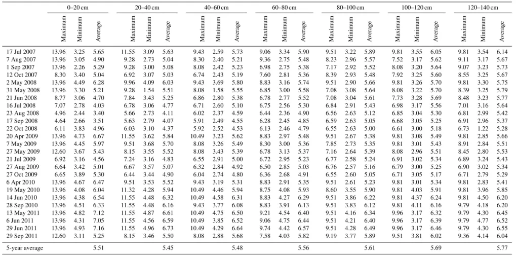
Average SWS for the surface 0–20 cm layer over the 5-year period was 5.51 cm. A slight decrease in SWS was ob-served at the immediate deep layer (20–40 cm) and a grad-ual increase thereafter. The 5-year average SWS was 5.45, 5.48, 5.56, 5.61, 5.69, and 5.77 cm for the 20–40, 40–60,
60–80, 80–100, 100–120, and 120–140 cm layers, respec-tively. Average SWS for a single measurement varied from 3.40 to 7.16 cm. The highest average SWS for the surface layer was observed on 29 June 2011. The study area re-ceived a large amount of spring snowmelt (2010 rere-ceived 642 mm, double the annual average precipitation) and rain-fall during 2011 leading to the high SWS in the surface layer (Weather Canada historical report). The lowest average SWS for the surface layer was observed on 23 August 2008, which was one of the driest summers within the 5-year study period. The highest average SWS (on 29 June 2011) at the surface layer gradually decreased to 6.55 cm at the deepest layer and the lowest average SWS (on 23 August 2008) at the surface layer gradually increased to 5.28 cm at the 120–140 cm layer (Table 1). These top and bottom boundaries formed a wider range (3.76 cm) of the average SWS at the surface layer com-pared to that at the deepest layer (1.27 cm). A big range (2.00 cm) in the standard deviation (maximum=2.43 cm and minimum=0.43 cm) of the measurement at the surface layer (0–20 cm) was also observed compared to that at the deepest layer (120–140 cm; maximum=1.28 and minimum=0.76). This indicated large variations in SWS at the surface layer that gradually decreased at deeper layers. The coefficients of variation (CVs) at the surface layer (0–20 cm) varied from 10 to 43 % and at the deepest layer (120–140 cm) varied from 13 to 23 % (Table S1 in the Supplement).
The maximum SWS at the surface layer also var-ied widely (maximum=13.96 cm and minimum=4.64 cm) compared to the deepest layer (maximum=9.81 cm and minimum=6.71 cm) (Table 1). There was a gradual decrease in the maximum value and increase in the minimum value from the surface to the deepest layer. The maximum SWS at different layers was more localized. For example, there was high SWS at different layers at the locations of 100 to 140 m and 225 to 250 m from the origin of the transect. These loca-tions had very high SWS compared to the field-average be-cause they were situated in the depressions while low SWS was observed on the knolls.
274
W
.
Ji
et
al.:
Fractal
beha
vior
of
soil
water
storage
at
multiple
depths
Table 1.Maximum, minimum, and average soil water storage (cm) at different depths (20 cm increment) over the whole measurement period.
0–20 cm 20–40 cm 40–60 cm 60–80 cm 80–100 cm 100–120 cm 120–140 cm
Maximum Minimum Av
erage
Maximum Minimum Av
erage
Maximum Minimum Av
erage
Maximum Minimum Av
erage
Maximum Minimum Av
erage
Maximum Minimum Av
erage
Maximum Minimum Av
erage
17 Jul 2007 13.96 3.25 5.65 11.55 3.09 5.63 9.43 2.59 5.73 9.06 3.34 5.90 9.51 3.22 5.89 9.81 3.55 6.05 9.81 3.54 6.14 7 Aug 2007 13.96 3.05 4.90 9.28 2.73 5.04 8.30 2.40 5.21 9.36 2.75 5.48 8.23 2.96 5.57 7.52 3.17 5.62 9.11 3.17 5.67 1 Sep 2007 13.96 2.26 5.29 9.28 3.00 5.08 8.08 2.42 5.23 6.98 2.75 5.38 7.17 2.92 5.52 8.08 3.20 5.64 9.07 3.23 5.73 12 Oct 2007 8.30 3.40 5.04 6.92 3.07 5.03 6.74 2.43 5.19 7.60 2.81 5.36 8.39 2.93 5.48 7.92 3.25 5.60 8.55 3.25 5.67 2 May 2008 13.96 4.49 6.28 9.96 4.09 6.03 9.43 3.69 5.80 8.83 3.16 5.74 9.51 2.90 5.66 9.81 3.26 5.70 9.81 3.30 5.75 31 May 2008 13.96 3.30 5.21 9.28 1.54 5.51 8.08 1.58 5.55 6.85 3.00 5.58 7.08 3.08 5.64 8.08 3.22 5.70 8.39 3.25 5.79 21 Jun 2008 8.77 3.06 4.70 7.84 3.43 5.25 6.86 2.80 5.38 6.78 2.77 5.52 7.08 3.04 5.61 7.73 3.28 5.69 8.48 3.23 5.77 16 Jul 2008 7.07 2.78 4.03 6.78 3.06 4.77 6.71 2.60 5.10 6.75 2.56 5.30 6.84 2.91 5.43 6.98 3.17 5.56 7.01 3.16 5.64 23 Aug 2008 4.96 2.44 3.40 5.66 2.73 4.11 6.02 2.37 4.59 6.44 2.36 4.90 6.56 2.63 5.12 6.85 3.04 5.30 6.81 2.99 5.42 17 Sep 2008 4.64 2.66 3.51 5.63 2.79 4.07 5.91 2.49 4.55 6.28 2.45 4.85 6.59 2.63 5.05 6.68 3.05 5.25 6.91 2.96 5.37 22 Oct 2008 6.11 3.83 4.96 6.03 3.10 4.37 5.92 2.52 4.53 6.13 2.46 4.79 6.55 2.63 5.00 6.61 3.00 5.18 6.73 1.22 5.28 20 Apr 2009 13.96 4.73 6.67 11.55 3.62 5.84 10.49 3.23 5.62 8.83 2.97 5.48 9.51 2.67 5.38 9.81 3.08 5.49 9.81 2.85 5.66 7 May 2009 13.96 4.45 5.97 9.51 3.68 5.70 8.08 3.26 5.49 8.30 3.00 5.36 7.85 2.73 5.35 9.81 3.01 5.43 8.91 2.84 5.51 27 May 2009 12.60 3.67 5.43 8.15 3.55 5.52 8.08 3.43 5.39 6.78 3.13 5.37 7.16 2.64 5.39 8.08 2.96 5.51 8.45 2.80 5.53 21 Jul 2009 6.92 3.16 4.56 7.24 3.16 4.83 6.55 2.91 5.00 6.72 2.95 5.23 6.77 2.58 5.24 6.91 3.02 5.34 6.89 3.24 5.43 27 Aug 2009 6.64 3.42 5.01 6.67 3.57 5.07 6.32 2.84 4.92 6.50 2.85 5.03 6.76 2.57 5.16 6.79 3.00 5.25 6.90 3.02 5.34 27 Oct 2009 6.65 3.89 5.30 6.44 3.44 4.90 6.04 2.74 4.80 6.36 2.68 4.91 6.55 2.60 5.05 6.71 3.05 5.17 6.71 2.79 5.29 6 Apr 2010 13.96 4.67 6.47 9.51 3.53 5.52 9.43 3.19 5.31 8.83 2.91 5.35 9.51 2.61 5.23 9.81 3.01 5.34 9.81 2.83 5.41 19 May 2010 13.96 4.08 6.04 11.32 4.28 5.94 10.49 4.46 5.94 8.75 4.08 5.93 8.60 3.55 5.90 9.81 4.03 5.91 9.81 3.96 5.85 14 Jun 2010 13.96 4.38 6.54 11.55 4.48 6.32 10.49 4.58 6.31 8.83 4.27 6.29 9.51 3.86 6.22 9.81 4.37 6.24 9.81 4.50 6.20 28 Sep 2010 13.96 4.51 6.33 11.55 4.48 6.16 9.43 3.77 6.08 8.83 3.91 6.13 9.51 3.83 6.12 9.81 4.11 6.16 9.79 4.18 6.20 13 May 2011 13.96 4.82 7.12 11.55 4.87 6.61 10.49 4.75 6.50 9.21 4.54 6.40 9.51 4.16 6.34 9.96 3.17 6.32 9.79 4.30 6.45 6 Jun 2011 13.96 4.31 7.05 11.55 4.56 6.59 10.49 3.85 6.52 9.06 4.75 6.44 9.51 4.21 6.40 9.96 3.17 6.39 9.79 4.77 6.52 29 Jun 2011 13.96 4.93 7.16 11.55 4.96 6.73 10.49 4.29 6.64 9.74 4.42 6.57 9.51 4.28 6.49 9.96 3.17 6.46 9.79 4.30 6.55 29 Sep 2011 12.60 3.11 5.25 8.15 3.46 5.50 8.08 2.88 5.68 7.58 4.03 5.82 9.19 3.77 5.89 9.51 3.81 6.02 9.36 4.14 6.04
5-year average 5.51 5.45 5.48 5.56 5.61 5.69 5.77
Nonlin.
Pr
ocesses
Geoph
ys.,
23,
269–
284
,
2016
www
.nonlin-pr
ocesses-geoph
Figure 2.Log–log plot between the aggregated variance of the SWS spatial series and the scale. A linear relationship indicated the presence of scale invariance and scaling laws for three selected dates.
The average water storage for soil layers with increasing depth was also calculated by adding the individual layers to-gether. The time-averaged values of SWS were 10.96, 16.44, 22.00, 27.61, 33.30, and 39.07 cm for the 0–40, 0–60, 0–80, 0–100, 0–120, and 0–140 cm, respectively (Table S2). The CV of the 0–20 cm layer was the highest during the wet pe-riod and gradually declined to the smallest during the dry period (Table S3). The variability also gradually decreased with depth.
3.2 Statistical scale invariance
The power-law relationships and the statistical scale invari-ance were evaluated using a log–log plot of the aggregated variance of SWS spatial series at different depths of soil lay-ers and the level of disaggregation (or scales) at different
276 W. Ji et al.: Fractal behavior of soil water storage at multiple depths
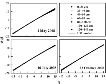
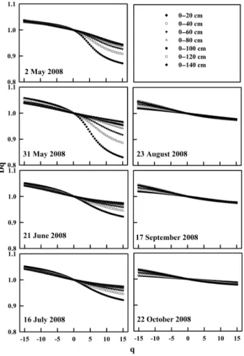
Figure 3.Mass exponents for soil water storage spatial series mea-sured at selected 20 cm soil layer down to 140 cm in 2008 for a range ofq(−15 to 15 at 0.5 increments). The solid line is a linear reference created following the UM model of Schertzer and Love-joy (1987) passing through (q=0).
linear fit (n=7) was between 0.99 and 1.00 (significant at
P =0.001) for any measurement days and depths. A simi-lar trend in scale invariance was also observed for SWS with increasing depth.
3.3 Multifractal analysis
The τ (q) curves for the surface layer displayed deviation from the UM model during the wet period (Fig. 3). A high SSR value was observed between the τ (q) curves and the UM model. Nonlinearity in the τ (q) curve was observed and the slopes of the segmented fit of the τ (q) curves were significantly different from each other. For exam-ple, the SSR values between the τ (q) curve and the UM model were 27.74 and 50.49 for the surface layer (0–20 cm) on 2 and 31 May 2008, respectively. The slopes of the
τ (q)curve for single fit were 0.97 and 0.96, respectively, for the surface layer of 2 and 31 May 2008 (Fig. 3). The slopes of the segmented fit for these measurements were 1.04 (q <0) and 0.87 (q >0) and, 1.06 (q <0) and 0.82 (q >0), respec-tively (Fig. 3; Table S4).
With the maximum deviation at the surface layer, the
τ (q)curves gradually became very similar to the UM model with depth. The SSR value decreased considerably in deep layers. The slopes of theτ (q)curve (single fit) became al-most at unity with no significant difference with the UM model. There was no significant difference between the slopes of the segmented fit. For example, the SSR value was 6.17, 4.98, 8.80, 8.50, 8.86, and 6.16 respectively for the 20–40, 40–60, 60–80, 80–100, 100–120, and 120–140 cm layer of 2 May 2008. The slopes (single fit) for these lay-ers were 0.99, 1.00, 1.01, 1.01, 1.00, and 0.99, respectively
Figure 4.Mass exponents for selected soil water storage spatial series from surface to different soil layers (cumulative storage) at 20 cm increment down to 140 cm in 2008 for a range ofq(−15 to 15 at 0.5 increments). The solid line is a linear reference created following the UM model of Schertzer and Lovejoy (1987) passing through (q=0).
(Fig. 3). The slopes of the segmented fit were also very close to unity with no significant difference between them.
The SSR values gradually decreased and the slopes be-came almost at unity with increasing depth (Fig. 4). For ex-ample, the SSR values were 14.11, 9.31, 7.71, 6.86, 6.71 and 6.30 and the slopes (single fit) were 0.98, 0.99, 0.99, 1.00, 1.00, and 1.00, respectively, for 0–40, 0–60, 0–80, 0–100, 0–120, and 0–140 cm layer (Table S5). The slopes of the segmented fit for theτ (q)curve became almost the same as soil layers went deeper (Fig. 4). The linearity of
the τ (q) curves was gradually strengthened and the SSR
value gradually fell with the depth increase of soil layers at any time. A significant difference was observed between the slopes of theτ (q)curves in segmented fitting at the surface layer of the first three measurements in 2007 (Fig. S1 in the Supplement), two measurements in 2008 (Fig. 4), three mea-surements in 2009, and all meamea-surements in 2010 and 2011 (Fig. S2).
A decreasing trend in the SSR value was also observed over time within a year. During the dry period, the slopes (single fit and segmented fit) became almost at unity with no significant difference (Table S6). For example, the SSR value was 14.12, 8.25, 1.30, 1.46, and 0.52 and the slope was 0.99, 0.99, 1.00, 1.00, and 1.00, respectively, for the surface layer (0–20 cm) of 21 June 2008, 16 July 2008, 23 August 2008, 17 September 2008 and 22 October 2008 (Fig. 3). Similarly, a small SSR value and consistent slope were also observed at the deepest layer (120–140 cm). The SSR values of the 120–140 cm were 2.47, 2.47, 3.31, 3.44, and 4.57, respec-tively, for the measurements on 21 June 2008, 16 July 2008, 23 August 2008, 17 September 2008, and 22 October 2008
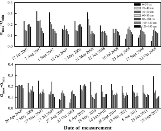
Figure 5.The width of the multifractal spectrum (αmax–αminvalue) for soil water storage at different depths (20 cm increment) for all measurements completed during the study period.
(Table S6). The slope (single fit) for all these measurements was equal to 1.01 (Fig. 3). There was very little difference in the slopes of the segmented fits.
A significant difference in the slopes of the segmented fit was observed for the surface layer (0–20 cm) of three mea-surements in 2007 (17 July, 7 August, and 1 September; Fig. S1), and three measurements in 2009 (21 April, 7 May, and 27 May) (Table S4; Fig. S2). The difference became non-significant with depth and during other measurement times. The trend in deep layers over time was very similar to that of 2008. However, the trend in the SSR values and the slopes with time was different in 2010 and 2011 (Table S6). There was very little difference in the SSR values at different times of the year. For example, the SSR value for the surface layer (0–20 cm) was 20.79, 27.18, 24.63, and 26.66 and the slope (single fit) was 0.97, 0.97, 0.97, and 0.97, respectively, for the measurements on 6 April 2010, 19 May 2010, 14 June 2010, and 28 September 2010 (Fig. 3). The slope of the segmented fit of the surface layer (0–20 cm) was significant for all mea-surements in 2010 and 2011. However, the trend with depth was similar to other years.
The height of the multifractal spectrum at different depths of measurement was very similar over time. The width of the spectrum (αmax–αmin) varied with depth and time (Fig. 5). Generally, a comparatively large value ofαmax–αminwas ob-served at the surface layer during the wet period and the value gradually became smaller with depth. For example,
the value ofαmax–αmin for the surface soil layer (0–20 cm) was 0.23 and 0.31, respectively, for the measurements of 2 and 31 May 2008 (Fig. 5). Meanwhile, the value ofαmax– αminfor the soil layers of 20–140 cm with 20 cm increment was 0.15, 0.14, 0.19, 0.20, 0.20, and 0.18 for 2 May 2008 and 0.25, 0.19, 0.11, 0.14, 0.12, and 0.11 for 31 May 2008, respectively (Fig. 6). In the later part of the year, the width of the spectrum gradually decreased (Table S8). For ex-ample, the αmax–αmin values were 0.19, 0.16, 0.07, 0.08, and 0.05, respectively for the surface layer on 21 June 2008, 16 July 2008, 23 August 2008, 17 September 2008 and 22 October 2008. Similar trend in values ofαmax–αminwas also observed at deep layers (Fig. 6).
278 W. Ji et al.: Fractal behavior of soil water storage at multiple depths
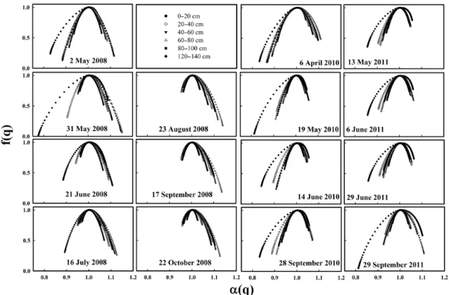
Figure 6.Multifractal spectra of soil water storage spatial series measured at each 20 cm soil layer down to 140 cm in 2008, 2010 and 2011 for a range ofq(−15 to 15 at 0.5 increments).
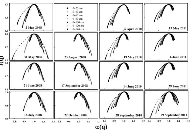
αmax–αmin was also small with the highest in the 0–20 soil layers and gradually decreased with depth (Fig. 7; Table S9). A very similar height of thef (q)curve for all depths and all periods indicated a consistent frequency distribution of the scaling indices (Figs. 6 and 7). Additionally, the posi-tion and the symmetry of the curve revealed the distribuposi-tion of scaling exponents. A symmetricf (q)curve indicated uni-form distribution of the scaling exponents. The left side of the spectrum corresponded to the large SWS that were amplified by the positive values ofq, whereas the right side indicated smaller SWS that were amplified by negativeqvalues. Sym-metry leaning towards the left side during the early spring and in the surface layers in 2008 clearly showed the wider distribution of scaling indices and multifractal nature of the SWS (Fig. 6). While the shifting of the symmetry towards the right side clearly indicated less variable scaling indices and thus reduction of multifractal behavior. During the wet years of 2010 and 2011, the symmetry towards the left side indicated the variability in the scaling indices. This also per-sisted with depth. A similar trend was observed for different years at all depth layers (Fig. 7).
Generally, the D1 andD2 values for different depths of different measurements were very close to 1 (Fig. 8 and Ta-ble S10). In general, theD1value of the surface layers gradu-ally increased with depth. Similarly, at any depth, theD1 val-ues gradually increased from the spring to the fall season through summer (Fig. 8). The highest variation inDvalues
withq was observed in the surface layer and in the spring season and gradually decreased with depth and later part of the growing season. For example, the first three measure-ments in 2007 and 2009 presented high D values at high
q values (Figs. S9 and S10). This high D value gradually decreased in the dry period of the year. For example, the
Dvalue with positiveqwas high in the surface layer of 2 and 31 May 2008 (Fig. 9), whereas it gradually decreased at the later part of the year (e.g., 17 September 2008). The trend with time and depth in 2007 and 2009 was very similar to that of 2008 (Tables S10 and S11). A consistently highDvalue was observed in the surface layer for all 2010 and 2011 mea-surements (Fig. 9). The trend inDvalues with depth in 2010 and 2011 was also similar to other years. A high value ofD1 andD2 were also observed at all depth layers for all mea-surements (Fig. 10; Table S11).
3.4 Joint multifractal analysis
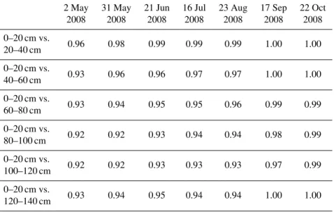
There were strong correlations between the scaling prop-erty of the joint distribution of the surface soil layer and the deep soil layers. The narrow width and the diagonally ori-ented contours between SWS measured on 22 October 2008 at 0–20 and 20–40 cm layers clearly demonstrate strong as-sociation between those two layers (Fig. 11). The correla-tion between the surface 0–20 cm and the deep layers on 2 May 2008 (wet period) was larger than 0.9 (significant at
P=0.001; Table 2). The highest correlation was observed
Figure 7.Multifractal spectra of soil water storage spatial series from surface to different soil layers (cumulative storage) at 20 cm increment down to 140 cm in 2008, 2010, and 2011 for a range ofq(−15 to 15 at 0.5 increments).
Figure 8.The information dimension (D1) for soil water storage at different depths (20 cm increment) over the whole measurement period.
between those layers closest to each other. The correlations gradually increased over time and showed high consistency between different layers on 17 September 2008 (Table 2). A very similar trend was observed in other years.
4 Discussion
280 W. Ji et al.: Fractal behavior of soil water storage at multiple depths
Table 2.Correlation coefficients between joint multifractal indices (αandβ) (n=440) of the surface layer with those from subsurface layers at 20 cm intervals in 2008.
2 May 31 May 21 Jun 16 Jul 23 Aug 17 Sep 22 Oct
2008 2008 2008 2008 2008 2008 2008
0–20 cm vs.
0.96 0.98 0.99 0.99 0.99 1.00 1.00
20–40 cm
0–20 cm vs.
0.93 0.96 0.96 0.97 0.97 1.00 1.00
40–60 cm
0–20 cm vs.
0.93 0.94 0.95 0.95 0.96 0.99 0.99
60–80 cm
0–20 cm vs.
0.92 0.92 0.93 0.94 0.94 0.98 0.99
80–100 cm
0–20 cm vs.
0.92 0.92 0.93 0.93 0.93 0.97 0.99
100–120 cm
0–20 cm vs.
0.93 0.94 0.95 0.94 0.94 1.00 1.00
120–140 cm
Figure 9.Generalized dimension spectra of soil water storage spa-tial series measured at each 20 cm soil layer down to 140 cm in 2008 for a range ofq(−15 to 15 at 0.5 increments).
winter months (Pomeroy et al., 2007). Generally, the de-pressions receive snow from surrounding uplands or knolls as redistributed by strong prairie wind (Pomeroy and Gray, 1995; Fang and Pomeroy, 2009). The snow melts within a short period of time during the early spring and contributes a large amount of water. The frozen ground restricts infil-tration and redistributes excess water within the landscape with greater accumulation in depressions (Fig. 1) (Gray et al., 1985). Apart from the snowmelt, the spring rainfall also contributes to the water inflow in the landscape (Fig. 1). This created a spatial pattern of SWS that was almost a mirror im-age of the spatial distribution of relative elevation (Biswas and Si, 2011a, c; Biswas et al., 2012a).
In the spring, the sources of water loss were the deep drainage and the evaporation. As the loss of water through deep drainage in the study area was as low as 2 to 40 mm per year, occurring mainly through the fractures and preferential flow paths (Hayashi et al., 1998; van der Kamp et al., 2003), the major loss occurred mainly through evaporation from the surface of the bare ground and standing water in depressions. These processes lose a very small amount of water compared to the input of water in spring and early summer leaving the soil wet. Moreover, the surface soil with high organic mat-ter content and low bulk density stored a larger amount of water than the deep layers where the organic matter grad-ually decreased and the bulk density increased. Reflecting the long-term history of vegetation growth in the landscape, the variability of organic matter content (CV=41 %) may be one of the main factors of the high variability in surface layer SWS (Biswas and Si, 2011b).
As the vegetation developed in summer, strong evapotran-spiration resulted in the lowest average SWS. High amounts of water in the depressions allowed grasses to grow faster and transpire more water compared to the knolls (Fig. 1).
Figure 10.Generalized dimension spectra of soil water storage spa-tial series from surface to different soil layers (cumulative storage) at 20 cm increment down to 140 cm in 2008 for a range ofq(−15 to 15 at 0.5 increments).
For example, the aquatic vegetation growth within the de-pressions was as high as 2 m, while the grasses on the knolls grew to a maximum of 1 m tall. The uneven growth of veg-etation and the high evapotranspirative demand in summer narrowed the range of SWS. In the soil where water is more available, evapotranspiration will be stronger while the less evapotranspirative demand will be shown in the relatively dry soil. As a result, the excessive water in the relatively wet soil will be offset by evapotranspiration, reducing the disparities between maximum and minimum values. This variable wa-ter uptake was visible in the growth of vegetation in the lawa-ter part of the growing season as well (Fig. 1). The reduction in the range of SWS was the largest in the surface layer and gradually decreased at deeper layers. This is because the sur-face layer was exposed to various environmental forces. For example, plants can take up more than 70 % of the water they need from the top 50 % of the root zone (Feddes et al., 1978). This dynamic behavior of the surface layer exhausted readily available water and finally reduced the range in water
stor-Figure 11.Multifractal spectra of joint distribution of SWS at 0– 20 and 20–40 cm measured on 22 October 2008. Contour lines show the joint scaling dimensions of the SWS measurement series.
age. This decrease in range also happened in the later part of the growing season.
282 W. Ji et al.: Fractal behavior of soil water storage at multiple depths
nature of the surface layer, and finally exhibited monofractal behavior in general.
The scaling patterns of SWS at different depths and peri-ods were further examined using multifractal spectrum [f (q)
vs.α(q)] (Figs. 6 and 7). The degree of convexity was used to characterize the heterogeneity of scaling exponents or the de-gree of multifractality. Large values ofαmax–αminindicated stronger heterogeneity in the local scaling indices of SWS or cumulative SWS and vice versa. The largest value for the surface layer(s) in the wet period indicated the most multi-fractal behavior of SWS. However, the value decreased with depth and gradually converged in deep layers (Fig. 6). This decline manifested a conformity in the scaling behavior of SWS at deeper layers. Over time, theαmax–αminvalue of the surface soil layer decreased and became very similar to that of deep layers. This indicated a reduction in the degree of multifractality for surface soil layers from the wet period to the dry period. A consistent αmax–αmin value for all depths during the dry period suggested the homogeneity and least multifractal nature of SWS. A similar behavior was observed in the cumulative SWS (Fig. 7).
To sum up, both the unity slope of theτ (q)curves (Figs. 3 and 4) and the degree of convexity of the f (q) spectrum (Figs. 6 and 7) jointly demonstrated that dynamic behavior of surface soil layers in the wet period made SWS highly variable and exhibited a multifractal nature, while less en-vironmental forces and increased buffering capacity of deep layers led to a monofractal nature. As a result, multiple scal-ing exponents were required to characterize the variability of SWS in the surface layer during the wet period, while a fewer number of exponents were necessary for deeper layers during wet period or all layers during dry period.
The height of the spectrum,f (q)revealed the dimension or frequency distribution of the scaling indices (Caniego et al., 2003). A low height off (q)curve indicated rare events or extreme values in the distribution, while a high value rep-resented uniform distribution in all segments. A very simi-lar height of the f (q) curve for all depths and all periods indicated a consistent frequency distribution of the scaling indices.
The two upper soil layers during the wet period tended to exhibit a longer tail of the curve on the left, showing more heterogeneity in the distribution of large values. However, when stepping into the dry period, the spectrum tended to display a longer tail on the right compared to the left side, suggesting more heterogeneity in the distribution of smaller values. A few locations with standing water lead to the spatial differences during the wet period, whereas a few points with very small SWS due to high evapotranspiration by growing vegetation during the dry period results in the heterogenic distribution in smaller values.
The generalized dimension, Dq was subsequently used
to characterize the scaling property and variability in SWS (Figs. 9 and 10). The largest value of f (q), referred to as the capacity dimension (D0) obtained atq=0, was close to
unity for all layers at different times (Fig. 9). The informa-tion dimension (D1) obtained atq=1 was different from the correlation dimension (D2), which is denoted as the average distribution density of the measurement for the surface layers in the wet period (Grassberger and Procaccia, 1983). In this case, the different values ofD0,D1, and D2 indicated the multifractal nature of the distribution of SWS. Similarly, a non-unity value ofD1/D0(Montero, 2005) also indicated the multifractal nature of SWS at the surface layer(s) during the wet period. However, over the growing season, theD1 and D2value approached toD0and indicated a monofractal type behavior. Similar values ofD0,D1, andD2 during the dry period also indicated homogeneous distributions.
Joint multifractal distribution between the surface to var-ious subsurface layers indicated the similarity in the scaling patterns (Table 2). Basically, the hydrological processes of shallower layers were similar to those of the top layer, while deeper layers showed more disparities from the surface. The nearest subsurface (20–40 cm) layer showed generally the highest similarity with the surface (0–20 cm) layer. However, in the wet period, the subsurface layers displayed the small-est similarity to the surface layer, suggsmall-esting a higher dy-namic nature of hydrological processes. In the dry period, a stronger effect of vegetation overwhelmed the effect of small variations of water distribution, thus creating a more uniform distribution of SWS at all soil layers (Table 2).
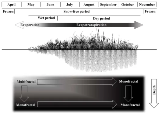
Overall, our result revealed a multifractal behavior of sur-face soil layers during the wet period due to the dynamic nature of hydrological processes. This behavior gradually changed with depth and time (Fig. 12). In the deeper layers during the wet period, the behavior became less multifractal or nearly monofractal. Similarly, in the dry period, the vege-tation development and its high evapotranspirative demand in the semi-arid climate of the study area increasingly buffered the variation of SWS, as a result, all the soil layers showed uniform distribution or monofractal behavior (Fig. 12).
5 Summary and conclusions
The transformation of information on soil water variability from one scale to another requires knowledge on the scal-ing behavior and the quantification of scalscal-ing indices. Sur-face soil water can be easily measured (e.g., remote sensing) and presents multi-scaling behavior (requiring multiple scal-ing indices). However, land-management practices require the understanding of the hydrological dynamics in the root zone and/or the whole soil profile.
In this manuscript, the scaling properties of soil water stor-age at different soil layers measured over a 5-year period were examined using multifractal and joint multifractal anal-ysis. The scaling properties of soil water storage mainly sug-gested a monofractal scaling behavior. However, the surface layer in the wet period or with high soil water storage tended to be multifractal, which gradually became monofractal with
Figure 12.Conceptual schematics showing vegetation development over time, dominant water loss processes and the scaling behavior of soil water storage at different depths. The figure is developed based on field observations and scaling analysis. The scale of the figure is arbitrary.
depth. With the decrease in soil water storage, the scaling be-havior became monofractal during the growing season. In a year with high annual precipitation, the soil stored more wa-ter in the surface layer throughout the growing period and displayed nearly multifractal scaling behavior. This multi-fractal nature indicated that the transformation of informa-tion from one scale to another at the surface layer during the wet period requires multiple scaling indices. On the contrary, the transformation requires a single scaling index during the dry period for the whole soil profile. The scaling properties of the surface layer were highly correlated with those of the deep layers, which indicated a highly similar scaling behav-ior in the soil profile. The study was conducted in an un-dulating landscape from a semi-arid climate and the results were very consistent over the years. Therefore, the observa-tion completed at the field scale in this type of landscape and climate may be generalized in similar landscapes and climatic situations, otherwise may need to be examined thor-oughly. The method used here can be transferred to examine the scaling properties in other experimental situations.
The Supplement related to this article is available online at doi:10.5194/npg-23-269-2016-supplement.
Acknowledgements. The project was funded by the Natural Science and Engineering Research Council of Canada. The help from the graduate student and the summer students of the Department of Soil Science at the University of Saskatchewan in collecting field data is highly appreciated.
Edited by: J. M. Miras Avalos Reviewed by: two anonymous referees
References
Biswas, A. and Si, B. C.: Scales and locations of time stability of soil water storage in a hummocky landscape, J. Hydrol., 408, 100–112, doi:10.1016/j.jhydrol.2011.07.027, 2011a.
Biswas, A. and Si, B. C.: Identifying scale specific controls of soil water storage in a hummocky land-scape using wavelet coherency, Geoderma, 165, 50–59, doi:10.1016/j.geoderma.2011.07.002, 2011b.
Biswas, A. and Si, B. C.: Revealing the Controls of Soil Wa-ter Storage at Different Scales in a Hummocky Landscape, Soil Science Society of America Journal, 75, 1295-1306, doi:10.2136/sssaj2010.0131, 2011c.
Biswas, A. and Si, B. C.: Identifying effects of local and nonlocal factors of soil water storage using cyclical correlation analysis, Hydrol. Process., 26, 3669–3677, doi:10.1002/hyp.8459, 2012. Biswas, A., Chau, H. W., Bedard-Haughn, A. K., and Si, B. C.:
Fac-tors controlling soil water storage in the hummocky landscape of the Prairie Pothole Region of North America, Canadian Journal of Soil Science, 92, 649-663, 10.4141/cjss2011-045, 2012a. Biswas, A., Cresswell, H. P., and Si, B. C.: Application of
Spa-284 W. Ji et al.: Fractal behavior of soil water storage at multiple depths
tial Variation: A Review, in: Fractal Analysis and Chaos in Geo-sciences, edited by: Ouadfeul, S.-A., InTech, Croatia, 109–138, 2012b.
Biswas, A., Zeleke, T. B., and Si, B. C.: Multifractal detrended fluc-tuation analysis in examining scaling properties of the spatial patterns of soil water storage, Nonlin. Processes Geophys., 19, 227–238, doi:10.5194/npg-19-227-2012, 2012c.
Caniego, F. J., Martí, M. A., and San José, F.: Rényi dimensions of soil pore size distribution, Geoderma, 112, 205–216, 2003. Chhabra, A. and Jensen, R. V.: Direct determination of thef (α)
singularity spectrum, Phys. Rev. Lett., 62, 1327–1330, 1989. Entin, J. K., Robock, A., Vinnikov, K. Y., Hollinger, S. E., Liu, S.
X., and Namkhai, A.: Temporal and spatial scales of observed soil moisture variations in the extratropics, J. Geophys. Res.-Atmos., 105, 11865–11877, doi:10.1029/2000jd900051, 2000. Evertsz, C. J. G. and Mandelbrot, B. B.: Self-similarity of harmonic
measure on DLA, Physica A, 185, 77–86, doi:10.1016/0378-4371(92)90440-2, 1992.
Fang, X. and Pomeroy, J. W.: Modelling blowing snow redistri-bution to prairie wetlands, Hydrol. Process., 23, 2557–2569, doi:10.1002/hyp.7348, 2009.
Feddes, R. A., Kowalik, P. J., and Zaradny, H.: Simulation of field water use and crop yield., John Wiley & Sons Inc., New York, 1978.
Grassberger, P. and Procaccia, I.: Characterization of Strange At-tractors, Phys. Rev. Lett., 50, 346–349, 1983.
Gray, D. M., Landine, P. G., and Granger, R. J.: Simulating infiltra-tion into frozen Prairie soils in streamflow models, Can. J. Earth Sci., 22, 464–472, 1985.
Grayson, R. B., Western, A. W., Chiew, F. H. S., and Bloschl, G.: Preferred states in spatial soil moisture patterns: Local and non-local controls, Water Resour. Res., 33, 2897–2908, 1997. Grego, C. R., Vieira, S. R., Antonio, A. M., and Della Rosa, S.
C.: Geostatistical analysis for soil moisture content under the no tillage cropping system, Scientia Agricola, 63, 341–350, 2006. Hayashi, M., van der Kamp, G., and Rudolph, D. L.: Water and
solute transfer between a prairie wetland and adjacent uplands, 2. Chloride cycle, J. Hydrol., 207, 56–67, 1998.
Hu, Z. L., Islam, S., and Cheng, Y. Z.: Statistical characterization of remotely sensed soil moisture images, Remote Sens. Environ., 61, 310–318, 1997.
Kachanoski, R. G. and de Jong, E.: Scale dependence and the tem-poral persistence of spatial patterns of soil water storage, Water Resour. Res., 24, 85–91, doi:10.1029/WR024i001p00085, 1988. Kim, G. and Barros, A. P.: Downscaling of remotely sensed soil moisture with a modified fractal interpolation method using con-traction mapping and ancillary data, Remote Sens. Environ., 83, 400–413, 2002.
Koster, R. D., Dirmeyer, P. A., Guo, Z. C., Bonan, G., Chan, E., Cox, P., Gordon, C. T., Kanae, S., Kowalczyk, E., Lawrence, D., Liu, P., Lu, C. H., Malyshev, S., McAvaney, B., Mitchell, K., Mocko, D., Oki, T., Oleson, K., Pitman, A., Sud, Y. C., Taylor, C. M., Verseghy, D., Vasic, R., Xue, Y. K., Yamada, T., and Team, G.: Regions of strong coupling between soil moisture and precipi-tation, Science, 305, 1138–1140, doi:10.1126/science.1100217, 2004.
Liu, H. H. and Molz, F. J.: Multifractal analyses of hydraulic conductivity distributions, Water Resour. Res., 33, 2483–2488, doi:10.1029/97WR02188, 1997.
Mandelbrot, B. B.: The fractal geometry of nature, W. H. Freeman and Company, San Francisco, 1982.
Mascaro, G., Vivoni, E. R., and Deidda, R.: Downscaling soil mois-ture in the southern Great Plains through a calibrated multifrac-tal model for land surface modeling applications, Water Resour. Res., 46, W08546, doi:10.1029/2009WR008855, 2010. Meneveau, C., Sreenivasan, K. R., Kailasnath, P., and Fan, M. S.:
Joint multifractal measures: Theory and applications to turbu-lence, Phys. Rev. A, 41, 894–913, 1990.
Montero, E. S.: Rényi dimensions analysis of soil particle-size distributions, Ecol. Model., 182, 305–315, doi:10.1016/j.ecolmodel.2004.04.007, 2005.
National Wetlands Working Group: The Canadian wetland classifi-cation system, University of Waterloo, ON, 1997.
Pomeroy, J. W. and Gray, D. M.: Snowcover, accumulation, reloca-tion, and management, in: NHRI Science Report No. 7, Environ-ment Canada, Saskatoon, SK, 144+xiii pp., 1995.
Pomeroy, J. W., de Boer, D., and Martz, L. W.: Hydrology and water resources, in: Saskatchewan: Geographic Perspectives, edited by: Thraves, B., CRRC, Regina, SK, Canada, 2007.
Quinn, P.: Scale appropriate modelling: representing cause-and-effect relationships in nitrate pollution at the catchment scale for the purpose of catchment scale planning, J. Hydrol., 291, 197– 217, doi:10.1016/j.jhydrol.2003.12.040, 2004.
Rodriguez-Iturbe, I., Vogel, G. K., Rigon, R., Entekhabi, D., Castelli, F., and Rinaldo, A.: On the spatial-organization of soil-moisture fields, Geophys. Res. Lett., 22, 2757–2760, doi:10.1029/95gl02779, 1995.
Schertzer, D. and Lovejoy, S.: Physical modeling and anal-ysis of rain and clouds by anisotropic scaling multiplica-tive processes, J. Geophys. Res.-Atmos., 92, 9693–9714, doi:10.1029/JD092iD08p09693, 1987.
Sivapalan, M.: Scaling of hydrologic parameterizations, 1. Simple models for the scaling of hydrologic state variables, examples and a case study, Center for Water Research, University of West-ern Australia, Nedlands, WA, Australia, 1992.
van der Kamp, G., Hayashi, M., and Gallen, D.: Comparing the hydrology of grassed and cultivated catchments in the semi-arid Canadian prairies, Hydrol. Process., 17, 559–575, doi:10.1002/hyp.1157, 2003.
Voss, R.: Fractals in nature: From characterization to simulation, in: The Science of Fractal Images, edited by: Peitgen, H.-O., and Saupe, D., Springer, New York, 21–70, 1988.
Western, A. W., Grayson, R. B., Bloschl, G., Willgoose, G. R., and McMahon, T. A.: Observed spatial organization of soil moisture and its relation to terrain indices, Water Resour. Res., 35, 797– 810, 1999.
Zeleke, T. B. and Si, B. C.: Scaling properties of topographic indices and crop yield: Multifractal and joint multifractal approaches, Agron. J., 96, 1082–1090, 2004.