General procedure to initialize the cyclic soil water balance by the Thornthwaite and Mather method

Note

General procedure to initialize the cyclic soil water balance by

the Thornthwaite and Mather method

Durval Dourado-Neto

1

_{; Quirijn de Jong van Lier}

2

_{; Klaas Metselaar}

3

_{; Klaus Reichardt}

4

_*;

Donald R. Nielsen

5

1

USP/ESALQ - Depto. de Produção Vegetal, C.P. 09 - 13418-900 - Piracicaba, SP - Brasil. 2

USP/ESALQ - Depto. de Ciências Exatas. C.P. 09 - 13418-900 - Piracicaba, SP - Brasil. 3

WUR - Dept. of Environmental Sciences, Postbus 47 - 6700AA - Wageningen - The Netherlands. 4

USP/CENA, Lab. de Física do Solo, C.P. 96 - 13400-970 - Piracicaba, SP - Brasil. 5

UCD - Dept. of Land, Air and Water Resources - 95616 - Davis, CA - USA. *Corresponding author <klaus@cena.usp.br>

ABSTRACT: The original Thornthwaite and Mather method, proposed in 1955 to calculate a climatic monthly cyclic soil water balance, is frequently used as an iterative procedure due to its low input requirements and coherent estimates of water balance components. Using long term data sets to establish a characteristic water balance of a location, the initial soil water storage is generally assumed to be at field capacity at the end of the last month of the wet season, unless the climate is (semi-) arid when the soil water storage is lower than the soil water holding capacity. To close the water balance, several iterations might be necessary, which can be troublesome in many situations. For (semi-) arid climates with one dry season, Mendonça derived in 1958 an equation to quantify the soil water storage monthly at the end of the last month of the wet season, which avoids iteration procedures and closes the balance in one calculation. The cyclic daily water balance application is needed to obtain more accurate water balance output estimates. In this note, an equation to express the water storage for the case of the occurrence of more than one dry season per year is presented as a generalization of Mendonça’s equation, also avoiding iteration procedures.

Key words: actual and reference evapotranspiration, deficit and excess water

Critério geral para iniciar o balanço hídrico pelo método

de Thornthwaite e Mather

RESUMO: O método original de Thornthwaite e Mather, proposto em 1955 para calcular o balanço hídrico semanal, é utilizado com freqüência devido à baixa exigência de dados de entrada e da obtenção de estimativas coerentes dos parâmetros do balanço. Como valor inicial para o início dos cálculos, geralmente assume-se que o armazenamento de água encontra-se na capacidade de campo ao fim do último mês da estação chuvosa. Ele será menor que a capacidade de campo em casos de climas áridos e semi-áridos. Para fechar o balanço, muitos ciclos iterativos podem ser necessários, o que pode ser complicado em muitas situações. Para climas áridos e semi-áridos com apenas uma estação seca, Mendonça desenvolveu em 1958 uma equação para quantificar o armazenamento no último mês da estação chuvosa, que permite fechar o balanço em um ciclo apenas. O balanço hídrico diário torna-se necessário para se obter estimativa de saídas mais precisas. Nessa nota, é apresentada uma rotina para expressar o armazenamento de água para o caso da ocorrência de mais de uma estação seca, uma situação que é bastante relevante quando é feito o balanço em escala diária, em regiões áridas e semi-áridas. Palavras-chave: evapotranspiração real e de referência, deficiência e excedente hídrico

Introduction

Climatologic soil water balance estimation is an important tool for edaphological characterization (Martin et al., 2008). Among the methods to estimate the soil water balance from simple soil and climate data, the method proposed by Thornthwaite and Mather (1955) is one of the most widely used. This procedure allows estimating the actual evapotranspi-ration, soil water deficit and excess. Therefore, it is especially useful for evaluating the effectiveness of agricultural practices (Dunne and Leopold, 1970;

Black, 1996; Silva et al., 2006; Bruno et al., 2007; Sparovek et al., 2007).

have used the original Thornthwaite and Mather’s model (Alley, 1984), while others have shown that this proce-dure can also be applied to smaller time scale (Eaton, 1995; Swanson, 1996), modifying the original model in an effort to improve certain components of the water balance. Steenhuis and Van Der Molen (1986) and Rushton et al. (2006) presented a study of the Thornthwaite’s method at a daily scale.

The uses of a monthly scale in water balance mod-els can, for example, lead to as much as a 25% underes-timate of groundwater recharge (Rushton and Ward, 1979). The recharge estimation tends to decrease if the time scale is lower. If the accounting period is longer than ten days, Howard and Lloyd (1979) also demon-strated that large errors could occur in the water bal-ance.

A modified Thornthwaite and Mather’s model was applied by Swanson (1996) in Wisconsin. The recharge was considerably lower than needed for the successful calibration of a regional groundwater flow model (Krohelski et al., 2000). One of the main explanations for the low estimates was related to the use of a monthly scale in the water balance calculations. Thornthwaite and Mather (1957) gave a brief example of a daily appli-cation, because this is needed for more accurate water balance output estimates. They reported that their pro-cedure could theoretically be used at a daily scale.

In this note, an equation that generalizes the ap-proach of Mendonça (1958) is proposed to determine the initial soil water storage without making use of itera-tions, for locations with more than one dry and wet sea-sons per year, a situation which becomes especially rel-evant in arid and semi-arid climates.

Theoretical background

The monthly cyclic water balance (Thornthwaite and Mather, 1955)

The basic equation to estimate the actual soil water storage (A, mm) is (Thornthwaite and Mather, 1955) (Ap-pendix A):

c C.e

L A

A A

−

= (1)

where L is the accumulated potential water loss (mm), defined as the accumulated sum of the difference be-tween pluvial precipitation (P, mm) and potential evapo-transpiration (ETo, mm) (equation 3) and A_C is the soil water holding capacity (mm):

A_C = (θ_f – θ_w)Z_e (2)

where Z_e is effective root depth (mm), θ_f and θ_w are, re-spectively, the field capacity and the wilting point soil water contents (cm3 _cm–3_).

If (Pi – EToi) < 0 (case I - dry season):

Li = Li–1 – (Pi –EToi) (3)

and

C C.e

A i L

i A

A

−

= (4)

If (P_i – ETo_i) ≥ 0 (case II - wet season):

Ai = Ai–1 + (Pi –EToi); if Ai ≥ AC then Ai = AC (5)

and

⎟⎟ ⎠ ⎞ ⎜⎜ ⎝ ⎛ − =

C C.ln

A A A

L i

i (6)

The actual evapotranspiration (

ETa

_i, mm), for the period i, can be computed as follows:

ΔAi = Ai – Ai–1 (7)

ETa_i = P_i + ΔA_i (8)

where ΔAi is the soil water storage change between the

periods i and i-1.

The soil water deficit (D, mm) and excess (E, mm) can be calculated as follows:

case I (dry season):

Di = EToi – ETai (9)

E_i = 0 (10)

case II (wet season):

D_i = 0 (11)

Ei = Pi – EToi – ΔAi (12)

Procedures to estimate soil water storage at the end of the wet season

Thornthwaite and Mather (1955)

conver-gence of the monthly values of soil water storage is reached leads to an inconvenient calculation routine.

Mendonça (1958)

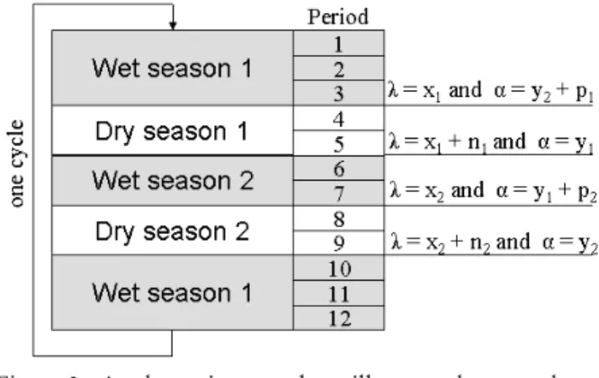
To avoid the need of the iterative computing proce-dure described above for the case of a dry climate, Mendonça (1958) proposed a procedure (Figure 2) to ini-tialize the cyclic monthly soil water balance for those cases in which one wetter season can be identified. Us-ing the expressions:

α = e–λ ₍₁₃₎

with

C

α A

A

= (14)

C

λ A

L

= (15)

A system of two equations and two unknown vari-ables x and y (Figure 2) can be written based on equa-tions (13), (14) and (15):

x

p

y

+

=

e

− (end of wet season) (16) (x n)

y

=

e

− + (end of dry season) (17)

where y is A per unit of A_C (y = α) in last month of the dry season, x is L per unit of AC (x = λ) in the last month

of the wet season, and Ld, Lw, n and p are defined as:

(

)

d i i

L P ETo

b

i a=

= −

∑

− ; if (P_i – EToi) < 0 and b ≥ a (18)

(

)

(

)

12

d i i i i

1

L P ETo P ETo

b

i a= i=

= −

∑

− −

∑

− ; if (P_i – ETo_i) < 0

and if b < a (18a)

(

)

(

)

12 1

w i i i i

1 1

L P ETo P ETo

a

i b i

−

= + =

=

∑

− +

∑

− ; if (P_i – ETo_i) ≥ 0 and

if b ≥ a (19)

(

)

1

w i i

1

L P ETo

a

i b

−

= +

=

∑

− ; if (P_i – ETo_i) ≥ 0 and if b < a: (19a)

d C

L n

A

= (20)

w C

L p

A

= (21)

where a and b are the numbers of order of the first and the last month of the dry season, respectively.

To estimate L in the last month of the wet season of a cyclic monthly soil water balance, Mendonça (1958) proposed:

Cln .

1 -n C

p

L A . A x

- e

⎛ ⎞

= − _{⎜ ⎟}= −

⎝ ⎠ (22)

This equation allows L to be obtained in a straight-forward way whereas it would take several cycles to find L by convergence using the original Thornthwaite and Mather procedure.

The proposed procedure

A general procedure is proposed analogous to the Mendonça procedure, but for cases where more than one dry and wet seasons can be identified, irrespective of the time step within the period considered for analysis. This approach becomes relevant especially when using daily or weekly time scales (calculation steps, input data). The general equation to define L at the last period of the first wet season, in case of two (Figure 3) and three (Figure 4) dry and wet seasons, allowing the computation of soil water storage at the first period of the subsequent dry season are, respectively (Appendix B and C):

( ) ⎥ ⎦ ⎤ ⎢

⎣ ⎡

− + −

= _{− +}−

2 1

2

1 . ln

. 1 2

C n n

n

e e p p A

L (two dry seasons) (23)

and

( )

( ) ⎥

⎦ ⎤ ⎢

⎣ ⎡

−

+ +

−

= −₋ +_{+ +} −

3 2 1

3 3

2

1

. .

ln

. 1 2 3

C n n n

n n

n

e

e p e

p p A L

(three dry seasons) (24)

Figure 1 - A schematic example of the Thornthwaite and Mather’s (1955) procedure to initialize the cyclic monthly soil water balance.

⎟⎟ ⎟ ⎟ ⎟ ⎟

⎠ ⎞

⎜⎜ ⎜ ⎜ ⎜ ⎜

⎝ ⎛

∑ ∑ +

− =

= = −

=

∑

k

i i j

j

n

i i C

e p A

L

1 i

n -k

2 1

e -1

. p

.ln _{(k ≥ 1) (25)}

If k = 1, equation (25) reduces to equation (22) as proposed by Mendonça (1958) for just one dry season (Table 1).

Results and Discussion

The application of the Thornthwaite and Mather (1955) procedure to initialize the climatic cyclic soil wa-ter balance (L = 0 mm) (Tables 2 and 4, with one wet season in March; and Tables 3 and 5, with two wet

sea-Using the Mendonça (1958) procedure (ME) (Table 1), for the case of a single dry period in Petrolina (Table 2 and 4), the accumulated potential water loss (L, mm) at the end of the last month of the wet season is calcu-lated directly using parameters shown in Table 6. Us-ing the proposed procedure (PP) (Table 1, equation 25), the accumulated potential water loss (L2, mm) at the

on-set of the first dry season (February) is calculated di-rectly (Table 7).

The Thornthwaite and Mather (1955) soil water bal-ance method is popular in regions with low data avail-ability. To apply this method in dry climates, an initial

Table 1- Procedures (Thornthwaite and Mather - TM, Mendonça - ME, and the proposed procedure - PP) to estimate initial parameters for a cyclic soil water balance based on the Thornthwaite and Mather (1955) method, defining the accumulated potential water loss L at the last period of the wet season.

e r u d e c o r

P Numberofseasons Equationforaccumulatedpotentialwaterloss Equation# Figure#

M

T k L_{=0 - 1}

E

M 1 22 2

P

P 2 23 3

P

P 3 24 4

P

P k _{25 5}

⎟ ⎠ ⎞ ⎜ ⎝ ⎛ −

= _-n

-e p . A L

1 ln

C

( ) ⎥ ⎦ ⎤ ⎢

⎣ ⎡

− + −

= _{− +}−

2 1

2

1

ln 1 2

C n n

n

e .e p p . A L

( )

( ) ⎥

⎦ ⎤ ⎢

⎣ ⎡

− + +

−

= _{− + +}

− +

−

3 2 1

3 3

2

1

ln 1 2 3

C n n n

n n

n

e

.e p .e

p p . A L

1

C

k k

exp 2 ln

k 1 exp

1

p p . n

i j

i j i

L A .

- - n

i i

⎛ ⎛ ⎞⎞

⎜ + ∑ ⎜− ∑ ⎟⎟

⎜ ₌ ⎜ ₌ ⎟⎟

⎝ ⎠

⎜ ⎟

= −

⎛ ⎞

⎜ ⎟

∑

⎜ ⎟

⎜ _{⎜ ⎟} ⎟

⎜ ⎝ = ⎠ ⎟

⎝ ⎠

Figure 4 - A schematic example to illustrate the procedure of beginning the cyclic soil water balance, for arid and semi-arid areas, with three dry seasons.

Table 2 The Thornthwaite and Mather procedure to initialize the climatic cyclic soil water balance (one wet season -March). Petrolina-PE, Brazil (period: 1975 to 2006).

ET₀: reference evapotranspiration (mm); P: pluvial precipitation (mm); L: accumulated potential water loss (mm); A: soil water storage (mm); Ac = 125 mm (soil water holding capacity).

h t n o

M P-ET0

0 L A

1 n o i t a r e t

I Iteration2 Iteration3 Iteration4

L A L A L A L A

J -70.9 921.3599 0.0787 1320.0009 0.0032 1321.2054 0.0032 1321.2059 0.0032

F -52.9 974.2605 0.0515 1372.9014 0.0021 1374.1059 0.0021 1374.1064 0.0021

M 5.1 0.0000 125.0000 398.6409 5.1510 399.8455 5.1016 399.8460 5.1016 399.8460 5.1016

A -42.4 42.4423 89.0124 441.0832 3.6680 442.2878 3.6328 442.2883 3.6328

M -78.8 121.2242 47.3952 519.8652 1.9531 521.0697 1.9343 521.0702 1.9343

J -97.8 219.0062 21.6773 617.6471 0.8933 618.8516 0.8847 618.8521 0.8847

J -94.8 313.7881 10.1554 712.4290 0.4185 713.6336 0.4145 713.6341 0.4145

A -103.8 417.5700 4.4271 816.2110 0.1824 817.4155 0.1807 817.4160 0.1807

S -118.4 536.0123 1.7164 934.6532 0.0707 935.8578 0.0700 935.8583 0.0700

O -142.3 678.2856 0.5499 1076.9265 0.0227 1078.1310 0.0224 1078.1315 0.0224

N -113.3 791.5588 0.2222 1190.1998 0.0092 1191.4043 0.0091 1191.4048 0.0091

D -58.9 850.4594 0.1387 1249.1003 0.0057 1250.3048 0.0057 1250.3053 0.0057

∆L₃ -398.6409 -1.2045 -0.0005 0.0000

h t n o

M P-ET0

0 L A

1 n o i t a r e t

I Iteration2 Iteration3 Iteration4

L A L A L A L A

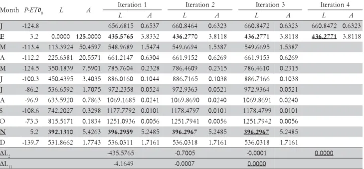
J -124.8 656.6815 0.6537 660.8464 0.6323 660.8472 0.6323 660.8472 0.6323

F _3.2 0.0000 125.0000 435.5765 _3.8332 436.2770 _3.8118 436.2771 _3.8118 436.2771 _3.8118

M -113.4 113.3924 50.4597 548.9689 1.5474 549.6694 1.5387 549.6695 1.5387

A -112.2 225.6381 20.5571 661.2147 0.6304 661.9152 0.6269 661.9153 0.6269

M -124.5 350.1839 7.5901 785.7604 0.2328 786.4609 0.2315 786.4610 0.2315

J -100.3 450.4395 3.4035 886.0160 0.1044 886.7165 0.1038 886.7166 0.1038

J -86.2 536.6592 1.7075 972.2358 0.0524 972.9363 0.0521 972.9364 0.0521

A -96.9 633.5920 0.7863 1069.1685 0.0241 1069.8690 0.0240 1069.8691 0.0240

S -108.6 742.2027 0.3298 1177.7792 0.0101 1178.4797 0.0101 1178.4799 0.0101

O -73.3 815.5171 0.1834 1251.0936 0.0056 1251.7941 0.0056 1251.7942 0.0056

N _5.2 392.1310 _5.4263 396.2959 _5.2485 396.2967 _5.2485 396.2967 _5.2485

D -139.7 531.8662 1.7743 536.0311 1.7161 536.0318 1.7161 536.0318 1.7161

∆L₂ -435.5765 -0.7005 -0.0001 0.0000

∆L₁₁ -4.1649 -0.0007 0.0000

ET₀: reference evapotranspiration (mm); P: pluvial precipitation (mm); L: accumulated potential water loss (mm); A: soil water storage (mm); Ac = 125 mm (soil water holding capacity).

Table 3 - The Thornthwaite and Mather procedure to initialize the climatic cyclic water balance (two wet seasons – February and November). Petrolina-PE, Brazil (year: 1976).

accumulated potential water loss must be estimated which, according to Thornthwaite and Mather (1955) can be done in an iterative procedure. As this iterative method is quite cumbersome, we propose a straightfor-ward calculation procedure to calculate this initial ac-cumulated potential water loss; a similar equation had already been proposed by Mendonça (1958), but unlike his equation, the one we deduced allows to express the

J 27 142.9 72 1321.2059 0.0032 0.0 72.0 70.9 0.0

F 27 142.9 90 1374.1064 0.0021 0.0 90.0 52.9 0.0

M _{27 142.9 148} 399.8460 _{5.1016 5.1 142.9 0.0 0.0}

A 26 124.4 82 442.2883 3.6328 -1.5 8 53. 41.0 0.0

M 25 107.8 29 521.0702 1.9343 -1.7 30.7 77.1 0.0

J 25 107.8 10 618.8521 0.8847 -1.0 11.0 96.7 0.0

J 25 107.8 13 713.6341 0.4145 -0.5 13.5 94.3 0.0

A 25 107.8 4 817.4160 0.1807 -0.2 4.2 103.5 0.0

S 26 124.4 6 935.8583 0.0700 -0.1 6.1 118.3 0.0

O 28 163.3 21 1078.1315 0.0224 0.0 21.0 142.2 0.0

N 28 163.3 50 1191.4048 0.0091 0.0 50.0 113.3 0.0

D 27 142.9 84 1250.3053 0.0057 0.0 84.0 58.9 0.0

l a t o

T 26.3 1,578.2 609.0 609.0 969.2 0.0

T: air temperature (o_{C); ET}

0: reference evapotranspiration (mm); P: pluvial precipitation (mm); L: accumulated potential water loss

(mm); A: soil water storage (mm); ΔA: soil water storage change (mm); ET_a: actual evapotranspiration (mm); D: water deficit (mm); E: water excess (mm); A_c = 125 mm (soil water holding capacity).

*http://www.theweathernetwork.com/index.php?product=statistics&pagecontent=C03198.

h t n o

M T ETo P L A _∆A ET

a D E

J 27 143.5 19 660.8472 0.6323 -1.1 19.8 123.7 0.0

F 25 107.4 111 436.2771 3.8118 3.2 107.4 0.0 0.0

M 26 126.2 13 549.6695 1.5387 -2.3 15.1 111.1 0.0

A 26 124.5 12 661.9153 0.6269 -0.9 13.2 111.3 0.0

M 26 124.5 0 786.4610 0.2315 -0.4 0.4 124.2 0.0

J 25 103.1 3 886.7166 0.1038 -0.1 2.9 100.1 0.0

J 23 88.1 2 972.9364 0.0521 -0.1 2.0 86.2 0.0

A 24 97.4 1 1069.8691 0.0240 0.0 0.5 96.9 0.0

S 26 118.1 10 1178.4799 0.0101 0.0 9.5 108.6 0.0

O 26 122.9 50 1251.7942 0.0056 0.0 49.6 73.3 0.0

N _{27 134.7 140} 396.2967 _{5.2485 5.2 134.7 0.0 0.0}

D 27 145.3 6 536.0318 1.7161 -3.5 9.1 136.2 0.0

l a t o

T 25.5 1,435.8 364.2 364.2 1,071.6 0.0

T: air temperature (o_{C); ET}

0: reference evapotranspiration (mm); P: pluvial precipitation (mm); L: accumulated potential water loss

(mm); A: soil water storage (mm); ΔA: soil water storage change (mm); ET_a: actual evapotranspiration (mm); D: water deficit (mm); E: water excess (mm); A_c = 125 mm (soil water holding capacity).

*http://www.theweathernetwork.com/index.php?product=statistics&pagecontent=C03198.

Table 5 - Climatic cyclic water balance (two dry seasons) using the Thornthwaite and Mather method. Petrolina-PE, Brazil (year: 1976).

Ld(mm) Lw(mm) n p x L3(mm)

5 0 6 2 . 4 7

9 5.0995 7.7941 0.0408 3.1988 399.8460 n: accumulated potential water loss during the dry season (L_d, mm) per unit of soil water holding capacity (Ac, mm) (equation 20). p: accumulated potential water loss during the wet season (L_w, mm) per unit of soil water holding capacity (Ac, mm) (equation 21). x: accumulated potential water loss at the last period of the wet season (L₃, mm) per unit of soil water holding capacity (A_c = 125 mm) (equation 22).

References

Alley, W.M. 1984. On the treatment of evapotranspiration, soil moisture accounting, and aquifer recharge in monthly water balance models. Water Resources Research20: 1137-1149. Black, P.E. 1996. Watershed Hydrology. 2ed. CRC Press, Boca

Raton, FL, USA. 408p.

Bruno, I.P.; Silva, A.L.; Reichardt, K.; Dourado-Neto, D.; Bacchi, O.O.S.; Volpe, C.A. 2007. Comparison between climatological and field water balances for a coffee crop. Scientia Agricola 64: 215-220.

Dunne, T.; Leopold, L.B. 1970. Water in Environmental Planning. W.H. Freeman, San Francisco, CA, USA. 818p.

Eaton, T.T. 1995. Estimating groundwater recharge using a modified soil-water budget method. In: Proceedings of AWRA. Wisconsin Nineteenth Annual Conference AWRA, Middleburg, VA, USA, p.18.

Howard, K.W.F; Lloyd, J.W. 1979. The sensitivity of parameters in the Penman evaporation equations and direct recharge balance. Journal of Hydrology 41: 329-344.

Krohelski, J.T.; Bradbury, K.R.; Hunt, R.J.; Swanson, S.K. 2000. Numerical simulation of groundwater flow in Dane County, Wisconsin. Wisconsin Geological and Natural History Survey, Madison, WI, USA, p.31. (Bulletin 98).

Martin, T.N.; Dourado-Neto, D.; Storck, L.; Burael, P.; Santos, E.A. 2008. Regiões homogêneas e tamanho de amostra para atributos do clima no estado de São Paulo, Brasil. Ciência Rural 38: 690-697.

Mendonça, P.V.E. 1958. Sobre o novo método de balance hídrico de Thornthwaite e Mather. In: Congresso Luso-Espanhol Para El Progresso De Las Ciencias 24, [sn], Madrid, Spain. p.415-425. Rushton, K.R.; Eilers, V.H.M.; Carter, R.C. 2006. Improved soil moisture balance methodology for recharge estimation. Journal of Hydrology 318: 379-399.

Rushton, K.R.; Ward, C. 1979. The estimation of groundwater recharge. Journal of Hydrology 41: 345-361.

Silva, A.L.; Roveratti, R.; Reichardt, K.; Bacchi, O.O.S.; Timm, L.C.; Bruno, I.P.; Oliveira, J.C.M.; Dourado-Neto, D. 2006. Variability of Water Balance Components in a Coffee Crop Grown in Brazil. Scientia Agricola 63: 105-114.

Sparovek, G.; Jong Van Lier, Q.; Dourado-Neto, D. 2007. Computer assisted Köppen climate classification for Brazil. International Journal of Climatology 27: 257-266.

Steenhuis, T.; Van der Molen, W. 1986. The Thornthwaite-Mather procedure as a simple engineering method to predict recharge. Journal of Hydrology 84: 221-229.

Swanson, S.K. 1996. A comparison of two methods used to estimate groundwater recharge in Dane County, Wisconsin. M.Sc. Dissertation. University of Wisconsin, Madison, WI, USA.

Thornthwaite, C.W.; Mather, J.R. 1957. Instructions and tables for computing potential evapotranspiration and the water balance. Publication in Climatology 10: 185-311.

n₁ and n₂: accumulated potential water loss during the first and second dry seasons (Ld₁and Ld₂, mm) per unit of soil water holding capacity (Ac, mm) (equation 20). p1 and p2: accumulated potential water loss during the first and second wet seasons (Lw1and Lw2, mm) per unit of soil water holding capacity (Ac, mm) (equation 21). x₁ and x₂: accumulated potential water loss at the last period of the first and second wet seasons (L₂ and L₁₁, mm) per unit of soil water holding capacity (A_c = 125 mm) (equation 23).

d

L ₁(mm) Lw₁(mm) n₁ p₁ x₁ L₂(mm)

1 7 1 5 . 5 1

8 3.1795 6.5241 0.0254 3.4902 436.2771

d

L ₂(mm) Lw₂(mm) n₂ p₂ x₂ L₁₁(mm)

5 0 5 5 . 4 6

2 5.2429 2.1164 0.0419 3.1704 396.2967

Table 7 - Values of the auxiliary parameters (Ld₁, Ld₂, Lw₁, Lw₂, n₁, n₂, p₁, p₂, x₁ and x₂), the accumulated potential water losses in February and November (L₂and L₁₁, mm), for two wet seasons (k=2), using the proposed procedure (Table 5). Petrolina-PE, Brazil (year: 1976).

Figure 5 - A schematic example to illustrate the procedure of beginning the cyclic soil water balance, for arid and semi-arid areas, with k dry seasons.

The derivation of the basic equation of estimating the soil water storage

The Thornthwaite and Mather (1955) method is based on the following assumption (Figure 6):

C A A K. dt dB₌ [A1] where L K ETo T

= = [A2]

A = A_C – B [A3]

where L and B stand for the accumulated potential wa-ter loss (mm).

Substituting [A2] and [A3] in [A1] and rewriting in convenient form:

∫

∫

= T

C L C dt T.A L dB -B A ₀ 0 1 [A4]

The integral solution becomes:

( )

T C L C t T.A L -B A -0 0 1 ln = ⎥ ⎥ ⎦ ⎤ ⎢ ⎢ ⎣ ⎡ ⎟⎟ ⎠ ⎞ ⎜⎜ ⎝ ⎛ [A5] Then C A L Ce A A −

= [A6]

Appendix B

The proposed procedure for two dry and wet seasons

Applying equation (13) for the two dry and wet sea-sons case:

y₂ + p₁ = e–x1 _[B1]

y₁ = e–(x₁₊ n₁₎

[B2]

y₁ + p₂ = e–x₂

[B3]

y₂ = e–(x2+ n2) _[B4]

Combining the equations (B1) and (B2) and (B3) and (B4):

p₁ = e–x₁

– e–(x₂₊ n₂₎

[B5]

p₂ = e–x₂

– e–(x₁₊ n₁₎

[B6]

Rewriting the equations (B5) and (B6) in convenient forms:

e–x₁

– e–n₂

. e–x₂

= p₁ [B7]

–e–n₁

. e–x₁

+ e–x₂

= p₂ [B8]

Then, by Kramer's rule:

2 2

.

1 1 2

2 1 1 n n e p p p e p D − − + = −

= [B10]

1 1 . 1 1 2 2 1 2 n

n p p e

p e

p

D ₋ = + −

−

= [B11]

(1 2)

2 1 1 . 2 1 1 n n n x e e p p Dp D

e _{− +}

− −

− + =

= [B12]

(1 2)

1 2 1 . 1 2 2 n n n x e e p p Dp D

e _{− +}

− −

− + =

= [B13]

( ) ⎥ ⎦ ⎤ ⎢ ⎣ ⎡ − + − = _{− +}− 2 1 2 1 . ln 1 2

1 n n

n

e e p p

x (cf. eq. 22) [B14]

( )⎥ ⎦ ⎤ ⎢ ⎣ ⎡ − + − = _{− +}− 2 1 1 1 .

ln 2 1

2 n n

n

e e p p

x [B15]

Appendix C

The proposed procedure for three dry and wet seasons

Applying equation (13) for the three dry and wet sea-sons case:

y₃ + p₁ = e–x₁

[C1]

y₁ = e–(x₁₊ n₁₎

[C2]

y₁ + p₂ = e–x₂

[C3]

y₂ = e–(x₂₊ n₂₎

[C4]

y₂ + p₃= e–x₃

[C5]

y₃ = e–(x₃₊ n₃₎

[C6]

Combining the equations [C1] and [C2], [C3] and [C4] and [C5] and [C6]:

p₁ = e–x₁

– e–(x₃₊ n₃₎

[C7]

p₂ = e–x₂

– e–(x₁₊ n₁₎

[C8]

p₃ = e–x3_{– e}–(x2+ n2) _[C9] Rewriting the equations [C7], [C8] and [C9] in con-venient forms:

e–x₁

– e–n₃

. e–x₃

= p₁ [C10]

–e–n₁

. e–x₁

+ e–x₂

= p₂ [C11]

–e–n₂

. e–x₂

+ e–x₃

= p₃ [C12]

Then, by Kramer's rule:

(1 2 3)

2 1 3 1 1 0 0 1 0 1 n n n n n n e e e e

Dp − + +

− − − − = − − −

(2 3) 3 2 3 . . 1 0 1 0 3 2 1 3 2 1 1 n n n n n e p e p p e p p e p

D − + −

− − + + = − −

= [C14]

(1 3) 1

1 3 . . 1 0 0 1 1 3 2 3 2 1 2 n n n n n e p e p p p p e e p

D − − + −

− + + = − − = [C15]

(1 2) 2

2

1 _{. .}

0 1 0 1 2 1 3 3 2 1 3 n n n n n e p e p p p e p e p

D − + −

− − _{= + +} − − = [C16] ( ) (1 2 3)

3 3 2 1 1 . . 3 2 1 1 n n n n n n x e e p e p p Dp D

e _{− + +}

− + − − − + + =

= [C17]

( ) (1 2 3)

3 1 1 2 1 .

. 2 3

1 2 n n n n n n x e e p p e p Dp D

e _{− + +}

+ − − − − + + =

= [C18]

( ) (1 2 3)

2 2 1 3 1 .

. 2 3

1 3 n n n n n n x e p e p e p Dp D

e _{− + +}

− + − − − + + = = [C19] and ( ) ( ) ⎥ ⎦ ⎤ ⎢ ⎣ ⎡ − + + − = −₋ +_{+ +} − 3 2 1 3 3 2 1 . .

ln 1 2 3

1 n n n

n n n e e p e p p

x (cf. eq. 23) [C20]

( ) ( ) ⎥ ⎦ ⎤ ⎢ ⎣ ⎡ − + + − = − _{− + +} − + 3 2 1 3 1 1 1 . .

ln 1 2 3

2 n n n

n n n e e p p e p x [C21] ( ) ( ) ⎟⎟_⎠⎞ ⎜⎜ ⎝ ⎛ − + + − = − + _{− + +}− 3 2 1 2 2 1 1 . .

ln 1 2 3

3 n n n