Econ. Apl. vol.9 número3

C

OSTS

AND

BENEFITS

OF

ELIMINATING

CHILD

LABOUR

IN

B

RAZIL

*

Ana Lúcia Kassouf§ Peter Dorman¤ Alexandre Nunes de Almeida†

RESUMO

O objetivo deste estudo é calcular os custos e benefícios econômicos decorrentes da eliminação do trabalho infantil no Brasil. Na análise foram considerados os seguintes custos: custo de prover escolas públicas do ensino fundamental com um nível adequado de qualidade; custo de oportunidade de eliminar o trabalho infantil, isto é, o valor do trabalho da criança; e o custo de eliminar trabalhos perigosos e que possam causar danos psicológicos e/ou à saúde das crianças e jovens. Do lado do benefício, calculamos os ganhos econômicos resultantes de uma população mais educada e mais saudável, já que a eliminação do trabalho perigoso e o aumento do nível de escolaridade resultam em benefícios à saúde. Os custos somaram 7 bi-lhões de dólares e o valor obtido para os benefícios foi de 35 bibi-lhões de dólares PPP, mostrando que os be-nefícios superam os custos.

Palavras-chave:trabalho infantil, análise de custo e benefício, educação.

ABSTRACT

The objective of this research is to calculate the economic costs and benefits of the elimination of child la-bor in Brazil. The framework focuses on three sources of cost: the cost of providing education to all chil-dren in lieu of work, the cost of program interventions to alter attitudes and practices, and the opportunity cost of eliminating this work, i.e. the value of children’s labor. On the benefit side, it calculates economic gains from a more educated population and the economic advantages resulting from a healthier popula-tion, since both more widespread education and the elimination of hazardous or unsuitable work have prospective health benefits. The costs obtained are close to seven billion dollars PPP and the benefits is more than thirty five billion dollars PPP. It is clear from the results that benefits outweigh the costs.

Key words: child labor, cost and benefit analysis, education.

JEL classification: J0.

* The authors would like to thank the relevant comments of the anonymous referee and clarify that although not all the com-ments were incorporated in the data analysis, since we were restricted to the use of a specific methodology, we, as much as pos-sible, raised the possibilities of improving the calculations in each specific item as suggested by the referee.

§ Associate Professor at Esalq/ USP and researcher at Cepea. ¤ Professor of Economics at Evergreen State College.

1 I

Basu and Tzannatos (2003) point out that researches on child labor have reappeared lately due to the importance of human capital accumulation to decrease poverty and increase develop-ment that is discussed in the developdevelop-ment literature and the view that child labor is an impedidevelop-ment to education and therefore to economic progress.

Although some authors have made some efforts to model theoretically the allocation of chil-dren’s time between work, school and leisure (Rosenzweig, 1981; Basu and Van, 1998; Emerson and Souza, 2003 etc.) the majority of articles focus on the empirical determinants of child labor (Grootaert and Patrinos, 1998; Kassouf, 2002; Nielsen and Dubey, 2002 etc.), the impact of child labor on his/her academic performance or on his/her school frequency (Psacharopoulos, 1997;

Gunnarsson et al., 2004; Glewwe, 2004 etc.), or the impact of legislation on the reduction of child

labor (Moehling, 1999).

Even with the growing recent academic interest on child labor and the great number of papers discussing the topic, there was not a study computing the economic costs and benefits of the elimi-nation of child labor.

This present study is a component of an ILO-IPEC (International Labour Organization – International Programme on the Elimination of Child Labour) project that attempts to calculate the economic costs and benefits of the elimination of child labour in Brazil. The methodology fol-lowed here was developed by ILO and used for another 7 countries – Senegal, Kenya, Tanzania, Ukraine, Pakistan, Nepal and Philippines – in the world. This methodology is unique to all coun-tries and, therefore, restricted to the data availability of each country. In this sense, we are aware that different and possible better approaches could have been taken place to obtain estimates of the costs and benefits of eliminating child labour in Brazil, but we were unable to change approaches since we were restricted to the methodology developed. However, the great merit of this study is to be a pioneer work quantifying economic aspects of the costs and benefits of child labour eradica-tion. It will therefore serve as a reference to later improvements in the estimates.

Cost-benefit analysis (CBA) is, in principle, a complete decision tool. It requires the identifi-cation and monetization of all consequences resulting from a given course of action; if their sum is positive – the benefits outweigh the costs – the action is undertaken. If the sum is negative, the ac-tion is rejected. Although practiac-tioners of CBA recognize that decisions may need to be taken on non-economic grounds, nevertheless the comprehensiveness of the approach implicitly calls into question the notion of “missing” dimensions and has led to a degree of tension in the policy com-munity. In some decision contexts a CBAs mission to be comprehensive is not problematic, but in the realm of child labour it is. First, the relevant question is not whether to take action to eliminate child labour, since this decision was already taken by the adoption of Conventions 138 and 182. The question is, now that we have accepted this commitment, what are the economic consequenc-es? Second, consensus among CBA practitioners does not extend to the techniques for monetizing intangible and qualitative aspects of public policy, such as social and health outcomes. Indeed, there is doubt that even ideal methods could fully capture these dimensions, as their costs and

ben-efits are not reducible to individual preferences.1

It is an assumption of this study that many important benefits of the elimination of child la-bour, such as the enhanced opportunity for personal development and social inclusion, are resistant to economic quantification. As a result, no attempt will be made to accomplish this. For example, the strictly economic benefits from more widespread education – greater income for the individual,

more rapid economic growth for the society – will be estimated, but the cultural and social benefits will not. Thus, in a technical sense, this is not a CBA but a study of net economic costs (or bene-fits). It is not designed to tell us what decision to make, but to advise us of the economic costs and benefits of that decision.

This study poses three major questions:

• How do the aggregate economic benefits from the elimination of child labour compare to the aggregate economic costs?

• How are these costs and benefits distributed among the primary stakeholders in the effort against child labour, especially households of child workers relative to the national economy as a whole?

• How do the costs compare to the resources now deployed against child labour or available for use in the future?

Since costs are borne up front and benefits accrue over time, the elimination of child labour can be thought of as an investment, and this study is designed to provide an approximation of its rate of return. Should the costs outweigh the benefits, this would not mean that child labour should not be addressed, but that, taking into account all the economic aspects, there is a net cost to be borne. There are other benefits to the elimination of child labour that cannot be captured in economic terms, such as greater opportunities for personal development and social inclusion. No effort will be made to monetize such values. Nevertheless, the economic dimension is important for what it says about both the attractiveness and feasibility of removing children from unsuitable work. In particular, it will be useful to know how the costs of eliminating child labour compare to the resources of governments that can potentially be mobilized. By detailing the costs and benefits to local populations, national economies, and the global system, these and other relevant questions can begin to receive answers.

Modelling the elimination of child labour would appear to require an analysis of its causes. The economic and social determinants of child labour are still an unsettled topic of debate,

partic-ularly the relationship between “development” (itself a contested concept) and child labour.2 No

doubt, improvements in the level of GDP per capita, general reduction in poverty and the suppres-sion of unproductive informal-sector work all have contributions to make. Nevertheless, it is be-yond the scope of this study to address these issues. In light of these constraints, the study will abstract from future economic development at the national and global levels. No claims will be made regarding measures other than the elimination of child labour (and the expansion of educa-tion) that might achieve more rapid development, and no assumptions will be made concerning the impact that further development may or may not have. Instead, we envision the elimination of child labour as resulting from an expansion of targeted programmes:

• the provision of public education up to the level of lower secondary school at an acceptable level of quality;

• the funding of income transfer programmes targeted at education that effectively eliminate the economic barriers to school attendance on the part of low-income children;

• the proliferation of interventions to overcome (i) social and cultural barriers to school attendance and (ii) engagement in the worst forms of child labour; and

• the creation of sufficient monitoring and enforcement capacity to contravene residual demand-side pressure.

2 S

– N

H

S

(PNAD 1999)

The main source of information used in this study is a National Household Survey (PNAD –

“Pesquisa Nacional por Amostra de Domicílios”) undertaken by the Brazilian Geographical and Sta-tistical Institute (IBGE) in 1999. This survey includes more than 330 thousand individuals from the Northeast, Southeast, South, Central and the urban part of the North of Brazil. It has informa-tion on the participainforma-tion of children in the labour force from the age of five, in addiinforma-tion to data on household characteristics, individuals’ education, sex, race, age, wages, hours of work, non-earn-ings income etc..

Another source of information is the school census. Private and public schools at county, state

and federal level provide information once a year. Since 1995 the school principal answers a ques-tionnaire containing the following information: school identification, school infrastructure, general information about classroom and personnel, pre-school education, literacy courses, primary school, secondary school, youths and adults’ education, and technical education.

Information on expenditures and government programs were obtained through the Ministry of Education, Treasury Bureau, and the Ministry of Retirement and Social Assistance.

3 G

While the project is ambitious, the time frame is condensed, so the framework seeks a middle ground between completeness and simplicity. It focuses on three sources of cost – the cost of pro-viding a quality education to all children in lieu of work, the cost of programme interventions to alter attitudes and practices, and the opportunity cost of eliminating this work, i.e. the value of chil-dren’s labour. On the benefit side, it calculates economic gains from a more educated population and the economic advantages resulting from a healthier population, since both more widespread education and the elimination of hazardous or unsuitable work have prospective health benefits. Calculations are based, whenever possible, on direct measurements from sources such as national or local surveys and censuses. Where numbers have to be constructed or imputed, simpler methods are generally preferred to more complex ones.

trans-fers. Essentially, then, each wave consolidates the annual changes taking place according to the projections established in the model.

The formulas used to obtain the present values for each wave considered are:

where

The real discount rates used (r)were 2%, 4%, 5% and 6%, and the population growth rate (g)

is obtained from IBGE.

Finally, it should be added that, among the simplifying procedures adopted in this study, is that of modelling the elimination of child labour through the replication of proven interventions, abstracting from potential changes in the environment due to economic development or other background events. In light of this, the study should be regarded as a conditional baseline

predic-tion: if there were no other economic changes in the countries under study, if sufficient resources

were expended to eliminate child labour, and if these resources were utilized with maximal

effec-tiveness, as calibrated by past examples of best practice, then the following costs and benefits would be expected to ensue.

The use of micro-data allows detailed information and more precise estimates of the required computations. A problem emerges, however, for the rural area of the Northern region, where there are no data collected in PNAD due to access difficulties, except for the Tocantins State. Trying to solve the problem, values were estimated assuming that the percentage of working children, poor children, and children in hazardous work in the rural Northeastern region was the same as in the rural Northern region, since they are both poor regions. The population in the rural Northern re-gion, according to 2000 census is 26% of the rural Northestern region and so the values were im-puted from the rural NE to the rural N area. Following this approach, we observe estimates for the rural northern region, but not for the states of the rural northern region.

The analyses were performed separately by each state of Brazil and region in the rural and

ur-ban areas.3

C

Since the study abstracts from the macro forces associated with the prevalence of child labour (such as those incorporated in the notion of “development”), it focuses on a set of micro factors: the ability of individual households to absorb the cost of withdrawing children from work and/or send-ing them to school, the cost of providsend-ing access to schoolsend-ing of sufficiently high quality to merit full-time attendance, the cost of promotion and awareness-raising to overcome cultural and social barriers to ending child labour, and the cost of directly intervening in the worst forms of this la-bour, through monitoring and enforcement activities. In addition, we also consider the extra cost resulting from efforts to remove and rehabilitate children already engaged in these worst forms. In

3 Tables can be obtained upon request to the authors.

) 1 /( ) 1 ( 1 wave , of lue

Present va 5

a a

x

x = − −

) 1 /( ) 1 ( 2 wave , of lue

Present va x = xa5 −a5 −a

) 1 /( ) 1 ( 3 wave , of lue

Present va x = xa10 −a5 −a

) 1 /( ) 1 ( 4 wave , of lue

Present va x = xa15 −a5 −a

this section, the precise methods used to measure these costs will be discussed in the context of pre-vious research in these fields.

4 C

–

For children, the most compelling potential alternative to full time work is education. Mil-lions of children are engaged in full time work because a satisfactory alternative is not available to them: either there are no schools at all within a convenient distance, or the schools are of such low quality that parents cannot see the advantage of enrolling their children. Even if children do attend such sub-standard schools, they may not receive the benefits that ought to be available to them as a result of foregoing child labour. For these reasons, quality as well as quantity (and location) are central to education supply.

The first step is to ascertain the physical accessibility of primary (children from 7 to 10 years old) and lower secondary (children from 11 to 14 years old) education. Accessibility is a function of mobility, of course. In an area in which people travel mostly on foot the accessibility radius of a school is smaller than in one in which people can travel by other forms of transport. In addition, a degree of capacity sufficient to serve a portion of the relevant age cohort is not the same as that needed to serve all such children, including those not currently attending.

Second, how many children have access to some form of age-appropriate school, but lack

ac-cess to quality education? This is a difficult and controversial question to answer. There is no

uni-versally agreed-upon set of criteria for quality; different analysts have different approaches. Quality may not mean the same thing in one country as another, since the challenges set before the school system may differ. Moreover, any dividing line between “adequate” and “inadequate” quality is necessarily arbitrary, and observers may disagree about where it should be drawn. Despite these qualifications, we propose the following criteria:

• Pupil-to-teacher ratio: this should not exceed 40 for any school. (Thus a national average of 40 would presumably include many schools that fail to meet this standard.)

• Books and other materials: non-salary recurrent costs must not be less than 15% of overall recur-rent expenditure.

These measures have the advantage of not only identifying such quality gaps as may exist, but also providing a method for calculating the cost of closing them. Thus the formula for quality up-grade is:

Quality upgrade cost = salary cost to achieve minimum pupil-to-teacher ratio + non-salary costs.

These costs will be expressed on a unit basis, that is, per student in the relevant target population and separately for primary and lower secondary schools. In all such calculations, the projected growth rate of the target population over time will be taken into account, and discounting will be applied.

There remains the question, what is the unit cost of providing education of sufficient quality where none existed before? The most direct way to calculate this is to take the existing unit costs, recurrent and capital, of supplying education and add to it the upgrade costs outlined in the previ-ous paragraph.

teach-ers was limited, and efforts to expand this pool would require greater spending on recruitment and salaries. A similar effect would arise if marginal (socially excluded or disadvantaged) populations – the last groups to be brought into the school system – are more costly to educate.

The total cost of education on the supply side will then be obtained by adding the mentioned costs as:

Total additional costs = additional costs of achieving attendance rate 100% + additional costs of achieving pupil-teacher ratio of 40 + additional non-wage expenditure up to 15% of recur-rent expenditure + additional capital expenditure

4.1 Calculating the additional cost of achieving attendance rate 100%.

There are 1,208,542 children out of school from 7 to 10 years old and 743,204 from 11 to 14 years old, adding to a total of 1,951,746. Children in pre-school or day-care were considered to be out of school

This quantitative information is important, but does not offer an appropriate understanding of the problem dimension. To attend to such issue, we calculated the attendance rate, which is the proportion of children 7-10 and 11-14 years old in school. The states of the north and northeast of Brazil have the smallest rates, since those are the poorest regions of the country. Attendance rate for the 7-10 years old children is 86.9% in rural areas and 92.3% in urban areas, and for the 11-14 years old is 91.7% in rural and 95.8% in urban areas.

The proportion of children in school starts low with 78.5% of the 7 years old studying, in-creases up to 11 years old and then dein-creases. Although a relatively large percentage of children is in school, a large amount is not in the correct grade for his or her age. Observing Table 4.1.1, it is clear that a large percentage of 11 (27%), 12 (33%), 13 (40%) and 14 (45%) years old kids are be-hind their expected grade (in bold). That explains why attendance rate is larger for lower second-ary then primsecond-ary education. In reality, a lot of 11-14 years old kids are in school but still in primsecond-ary school, not in lower secondary.

Table 4.1.1 – Percentage of children, at each specific age, in different grade levels. Numbers in bold are for kids behind their expected grade for each age*

*It was assumed that a 1st _{grade is the correct one for children up to eight years old, to account for differences in the date of}

birth around the year. Likewise, 2nd _{grade is correct for 9 years old and so forth.}

7 anos 8 anos 9 anos 10 anos 11 anos 12 anos 13 anos 14 anos

1st _{grade 81.3 30.8 13.7 6.3 4.1 2.8 1.8 1.3}

2nd _{grade 17.4 57.2 30.4 14.1 9.0 6.1 3.4 2.0}

3rd _{grade 1.3 11.3 47.1 26.9 14.0 9.4 6.9 4.5}

4th grade 0.7 8.1 44.6 26.0 14.5 9.4 7.0

5th _{grade 0.8 7.3 40.0 26.8 18.8 13.7}

6th _{grade 0.8 6.2 34.2 23.6 16.4}

7th _{grade 0.6 5.7 31.4 21.8}

8th _{grade 0.6 4.4 29.7}

old years 14 -11 or 10 -7 children of

number total

school in old years 14 -11 or 10 -7 children of

number rate

To calculate the costs of providing education to accommodate all children out of school by 2020 it is necessary to have the unit costs of one year of education or the expenditure on education per capita. The source of these data is the National Treasure Bureau from the Finance Ministry and the Ministry of Education. Values, in 1999-dollar PPP (R$1.00 = $0.8 PPP in 1999), vary con-siderably by state. The largest expenditures are in Roraima and São Paulo states, while the smallest are in the states of the northeastern region (Pernambuco, Alagoas, Piauí etc.). Those expenditures come from a Government National Fund to improve primary and secondary schools (FUNDEF), a State Quota of Educational Salary (QUESE), and a National Fund for Educational Develop-ment (FNDE). Each state allocates 15% of basically four taxes (trade, export, state fund, county fund) to FUNDEF, and when a minimum amount per student is not reached ($215 PPP in 1999), federal government provides a complement. Usually, just a part of the money coming from FUN-DEF is used to pay teachers. By law a minimum of 60% of this fund has to be used to teacher’s sal-aries. The FNDE and QUESE, on the other hand, cannot be used to pay teachers. They provide additional sum of money to education as a way to improve its quality. The money from FNDE is used to purchase and distribute equipments, textbooks and school meals. The money from QUESE is used to construct buildings, to make repairs, to buy consumption materials etc. Those values, however, may still not represent the total expenditure with schools, since there are other non-federal programs to complement schools’ expenditures. To obtain the total expenditure per student per year, the total expenditure in the FUNDEF, FNDE and QUESE was divided by the number of enrolments, given by school census. For Brazil, the current expenditure per student per

year is $441.06 PPP.4

The 1,208,542 children out of school from 7 to 10 years old were divided in waves as: 1/3 of the children in 2005, 2/3 in 2010 and 3/3 in 2015. Likewise, 743,204 children from 11 to 14 years old were divided in waves as: 1/3 of the children in 2010, 2/3 in 2015 and 3/3 in 2020. Those num-bers were then multiplied by the school government expenditure per student per year to obtain the additional cost of achieving attendance rate 100%, discounting at different interest rates. The for-mula used is:

additional cost of achieving attendance rate 100% = number of children out of school ×

expen-diture/pupil

For the 7-10 and 11-14 years old, respectively, at a 5% interest rate, the additional cost for the 7-10 years old children is $716,911,323.10 and for the 11-14 years old is $358,313,836.14. Therefore, the total additional cost of achieving attendance rate 100% is $1,075,225,159.24.

Graph 4.1.1 shows per capital total cost to reach attendance rate 100% in each region and in Brazil, adding the waves, both children age groups and urban/rural areas. The rural cost for the northern region was estimated, as described before. The cost for Brazil is $551 PPP per child out of school. The southeastern region presented the largest cost, followed by the south. North and cen-tral of Brazil showed similar rates, and the smallest cost was observed in the northeast.

Graph 4.1.1 – Per capita total cost to reach attendance rate 100% in each region and in Brazil, adding the waves, both children age groups and urban/rural areas

4.2 Calculating the additional cost of achieving pupil-teacher ratio of 40

A measure of school quality is number of pupil per teacher. It is established that schools should have a maximum of 40 and 30 pupils per teacher in the primary and secondary school lev-els, respectively.

Hiring teachers is a way to decrease the pupil-teacher ratio. If that action is necessary, the costs related to the payment of teacher’s salaries would have to be computed. However, data show

that the pupil-teacher ratio is always below the required level, except for the 5th to 8th grade in the

urban areas, but even in this case it does not surpass 40 pupils per classroom. Therefore, the calcu-lations to obtain the additional cost of achieving pupil-teacher ratio of 40 are not necessary.

4.3 Calculating the additional non-wage expenditure up to 15% of recurrent expenditure

There is no specific data available to obtain the percentage spent on books and other materials (non-wage inputs) necessary to calculate school quality cost. To obtain a proxy for non-wage ex-penditures, the amount spent on the FNDE and QUESE school programs was divided by the sum of the expenditures in the three major educational government programs (FUNDEF, FNDE and QUESE). The amount of money coming from programs other than FUNDEF, i.e., not used to pay teachers, with respect to the total amount of education’s programs, is very close to 15% in Bra-zil, specifically 14.6%. Data show that the percentage is below 15% for the majority of states and, therefore, the cost to increase it up to 15% has to be computed. To this end, a total number of stu-dents is required.

There are 20 states, out of 26, with a current non-wage expenditure of less than 15% of overall recurrent expenditure in Brazil. The computations were done only for those 20 states, bringing their percentage up to 15% level. The formula used is:

Additional non-wage expenditure= recurrent expenditure per pupil×

number of students

Dividing the students in waves (2005/2010/2015 for the 7-10 and 2010/2015/2020 for the 11-14 years old children) and calculating the present value at a 5% interest rate, the additional cost for the

493,7

368,3

726,0

562,5

491,0

550,9

0 100 200 300 400 500 600 700 800

North Northeast Southeast South Central Brazil region

p

e

r

ca

p

it

a

co

st

(

$

P

P

P

)

× ⎟ ⎠ ⎞ ⎜

⎝

⎛ ₋

1 85%

on wages spent

7-10 children is $120,465,295.54 and for the 11-14 is $62,113,730.47. Therefore, the total additional cost of reaching 15% of overall recurrent expenditure is $182,579,026.21.

Graph 4.3.1 shows per capital total non-wage cost in each region and in Brazil, adding the waves, both children age groups and urban/rural areas. The per capita cost in Brazil is $8.7 PPP, similar to the south. The north has the largest cost, followed by central region. The southeast and northeast have the smallest per capita cost. So, the northern region is the one requiring more in-vestment to improve school quality.

Graph 4.3.1 – Per capita total additional non-wage expenditure up to 15% of recurrent expendi-ture in each region and in Brazil, adding the waves, both children age groups and ur-ban/rural areas

4.4 Calculating the additional capital expenditure

Gross enrolment ratio (GER) below 100% is used to indicate lack of school buildings. This measure is obtained by dividing the total number of students in primary and lower secondary school, independent of age, by the total number of children at the correct primary and lower sec-ondary school age, i.e.,

The GER provides an indication of the capacity of each level of the educational system, but a high ratio does not necessarily indicate a successful educational system as this ratio includes overa-ge and underaovera-ge enrolments. It can be assumed that when GER is above 100 there are enough school establishments for achieving the goal of universal coverage. The percentages, in Brazil, did not exceeded 100% only for the 11 to 14 years old children living in rural areas, with the exception of São Paulo and Federal District.

The additional capital expenditure cost was obtained only for the states where GER was be-low 100%. The formula used is:

Additional capital expenditure = number of additional new building × capital unit cost

or 24,94 2,90 5,50 8,55 14,41 8,69 -5 10 15 20 25 30

North Northeast Southeast South Central Brazil

region per c api ta c o s

t ($ P

where

number of pupils not covered by capital expenditure = total number of children 11-14 years old − enrolments in 5th to 8th grade

and

The information on the amount government did spend specifically on school buildings is not available. The total amount spent on the QUESE program was used as an approximation, since the money coming from this fund allows the construction of school buildings, the establishments’ maintenance, and the purchase of consumption materials, besides others.

Dividing the 11-14 years old students living in rural areas in waves (2010/2015/2020) and cal-culating the present value at a 5% interest rate, the additional cost is $19,282,786.18.

4.5 Total additional costs of education on the supply side

To obtain the total additional costs of achieving universal education in 1st to 8th grade, the

fol-lowing formula is used:

Total additional costs = additional costs of achieving attendance rate 100 + additional non-wage expenditure up to 15% of recurrent expenditure + additional capital expenditure

The total cost for the supply side, at 5%, for the primary school is $837,376,618.65 and for the lower secondary school is $439,710,352.78. Therefore, the total cost for the supply side of education is $1,277,086,971.43.

Graph 4.5.1 shows the costs of education on the supply side, i.e., the additional expenditure of achieving attendance rate 100%, reflecting the costs to include every child from 7 to 14 years old in school by 2020; the additional non-wage cost, necessary for improving school quality such that ev-ery establishment would be spent at least 15% of its non-wage expenditure in books and other in-formative material; and additional capital cost to build new school establishments, if necessary, to include every child that was out of school.

Reaching attendance rate 100% requires the largest amount of money among the costs of edu-cation on the supply side, with more than one billion dollar PPP. According to the methodology, to improve school’s quality it is necessary almost two hundred million dollars PPP and to build new school establishments near twenty million dollars PPP.

Additional capital expenditure =

# of pupils not covered by capital expenditure

×

total government expenditure

average number of students per school number of establish-ments in urban and rural areas

average number of

students per school =

number of students enrolled in 1st to 8th grade in rural areas

Graph 4.5.1 – Total costs of education on the supply side

5 O

Underlying the approach taken to education in this study is the assumption that there are oth-ers overriding factors that determine whether parents will choose to transfer their children from work to full time school attendance. First, education of sufficient quality must be readily available to them. This has been addressed in the previous section on the supply side of education. Second, they must be able to overcome the purely economic barriers to having their children engaged in study. This includes the direct cost of schooling, such as books and uniforms, but also, and espe-cially, the opportunity cost – the value of the work children might have to give up if they increase their school participation.

The opportunity cost of eliminating child labour is the value of this labour itself: to the chil-dren, to their households and to the larger community. Here is where controversies surrounding policy are joined. Those who would move more rapidly to oppose child labour see this cost as rela-tively manageable and dwarfed by the benefits of taking action. Those who would go slower be-lieve these costs to be quite large; they stress that well-intended actions by child labour activists may actually hurt those they are trying to help. For some with a rational choice perspective, there is an initial presumption that the opportunity costs must be substantial, since parents (from this viewpoint) are often seen to choose to put their children to work. If parents are economically ratio-nal, and if they care about the future well-being of their children, they must be calculating that the

benefits of child work exceed the benefits of reduced opportunities for education.5 Such debates

cannot be answered theoretically; they can only be illuminated by empirical evidence – which it is a purpose of this study to collect.

5.1 Calculating the opportunity cost of child labour

Children were considered working if they had a job in the period between 26 September 1998 and 25 September 1999 before the interview, i.e., if they had any job in a one year period before the survey, or if they produced food for self consumption, or worked in construction for their own use, or if they worked but they were not working because of vacation or health problems.

5 Of course, parents might wish to borrow in order to finance their children’s education but be credit-constrained, as considered above.

1.075,23

182,58

19,28

-200 400 600 800 1.000 1.200

Additional cost of attendance rate 100

Additional non-wage expenditure

Additional capital expenditure

cost of education - supply side

milli

ons of dollar

s

There are 2,299,586 children from 5 to 14 years old working in rural areas and 1,349,252 in urban areas of Brazil, adding to a total of 3,648,838.

To obtain the opportunity cost of children’s work, it is assumed that the wage children receive

is equal to their economic contribution, i.e., wage and productivity are the same.6 For children

working and receiving payment, it is a simple task to find their opportunity cost. However, if child labour is unpaid, it becomes more complicate to assign a value to its labour. Estimates can be ob-tained by using the value of the good produced and the share of time and wage children spend pro-ducing that good with respect to an adult. However, due to lack of data on the share of time attributed to child and adult per product or service, and on the amount of goods produced, child’s opportunity costs were calculated in the following way:

i. Separately for boys and girls, and using micro-data from PNAD 1999, if children were paid a sal-ary, the monthly salary was the value of their work.

ii. Total monthly salary was obtained adding the earnings from all jobs declared by the child, including any form of payment in-kind.

iii. Separately, for all female and male children, it was calculated the average monthly earnings for occupations related to domestic work, i.e., baby sitter, cleaner, cooker, cloth washer etc .

iv. If a child declared to be doing domestic work and was not studying, it was attributed a “domestic

servant” salary available to some employed children, obtained in item (iii). The reason for

con-sidering children not studying relates to the fact that, in this case, the probability that they would

be doing a full time household work is higher.7

It is essential to assign a monetary value to the household activities, because if children with-draw from their activities, either heads will have to accept a lower level of self-provision or they will have to hire people to do the tasks.

v. Salaries for boys and girls from 7 to 14 years old were then put together to find the average

opportunity cost per state/region and urban/rural areas.8

On average, children in urban area of Rio de Janeiro and São Paulo state, for example, will re-ceive 68% and 54% more ($83.49 and $73.70 per month) than relatively poor areas such as rural Alagoas or Tocantins ($49.76 and $47.82), respectively. This fact shows the importance of having income transfer programs differentiated by locality. A given amount of money, in areas where the opportunity cost is low, may allow a child to go to school and to stay there, but may not have an ef-fect on places where the opportunity cost is high.

Dividing the working children in waves (2005/2010/2015/2020 for the 7-14 years old children) and calculating the present value at a 5% interest rate, the additional cost is $3,625,659,597.87.

Graph 5.1.1 shows per capita opportunity cost of child labour for each region and in Brazil, adding the waves, and urban/rural areas. The per capita cost in Brazil is $994 PPP. The regions show similar rates of per capita cost, with southeast being the largest and northeast of Brazil the smallest among regions.

6 “In reality their wage may be more or less than this. It may be more because children are being taken on as a favor to their parents; it may be less because children are more intensively exploited as a result of their relative vulnerability and tendency to submit to authority. Unfor-tunately, we generally have no information on either possibility, and the best we can do is to assume that productivity and the wage are equal.” Extract from ILO, methodological framework for the global study on the costs and benefits of the elimination of child labour, 2002.

7 Information on number of hours spent in household activities is not available.

Graph 5.1.1 – Per capita total opportunity cost of child labour in each region and in Brazil, adding the waves, and urban/rural areas

6 C

Increasingly, analysts of child labour are coming to the view that some form of monetary transfers to low-income parents may be necessary to defray the explicit and implicit costs of

educa-tion.9A particularly innovative and successful set of programmes can be found in Brazil’s Bolsa

Es-cola. The study envisions that some version of Bolsa Escola will be adopted on a global basis. Local governments will target eligible households, calculate specific amounts to be transferred to each household, disburse the money and monitor the attendance of children. To do all this, an adminis-trative apparatus will need to be established.

For households whose income is below an appropriate poverty benchmark, we are assuming that an income transfer programme tied to school attendance will be required. The cost of this pro-gramme has two parts, its transfer and administrative components. The transfers depend on the ex-tent and depth of poverty and the productivity of child labour. To calculate the transfer costs we determine the appropriate level of income below which households will be classified as “poor” as well as the number of households qualifying as poor, and their average poverty gap (the additional income which would be required to bring them up to the poverty line). After that we determine the total number of children of school age (distinguishing primary from lower secondary) who are from poor households, and calculate the average number of such children for households in which there is at least one such child.

A hypothetical income transfer that replaces 80% of the opportunity cost of children’s work is then established, providing that this amount, multiplied by the average number of children per household, does not raise average household income (from all sources) above the poverty line. The

9 Such programmes are consistent with the view that a major barrier to the elimination of child labour is the inability of parents to borrow against the future economic benefits of have their children educated. For a recent analysis along these lines, see Ranjan (2001).

984

917

1.114

993 1.022 994

-200,00 400,00 600,00 800,00 1.000,00 1.200,00

North Northeast Southeast South Central Brazil region

pe

r c

a

p

ita

o

ppor

tunit

y

c

o

s

t (

$

P

P

P

gross transfer effected by the programme is obtained multiplying the estimated unit transfer by the number of children.

It is also necessary to calculate the value of existing income transfers delivered to poor

house-holds with school-age children that are not education-related. (These may be associated with

gen-eral transfer programmes that do not take account of the numbers and ages of children). The gross transfer minus these existing transfers yields the net transfer, which is the value of interest to the study.10

6.1 Calculating the additional cost of education – demand side

Households with per capita income equal or below half minimum salary per month (68.00 “reais” or 54.40 dollars PPP) were classified as poor. This poverty line is the same as the one used by the “bolsa escola” program. Households’ income includes salaries, earnings in-kind, rents, re-tirements, pensions, interests from savings etc. from all members of the household, except from household’s employees, employees’ relatives, renters and children below the age of 14. There are more than five million and a half households with 7 to 14 years old children below poverty line in Brazil, from which, 5,735,277 are poor children from 7 to 10 years old and 5,955,606 from 11 to 14 years old.

The additional average income that would be required to bring the households up to the

pov-erty line (gap) was multiplied by the number of household’s members, since we were using a per

capita value for the poverty line, which does not reflect the total necessary income to bring the whole household to poverty line level. The range goes from an average of $90.9 PPP (urban Rio de Janeiro) to $179.3 PPP (rural Piauí) per household.

To obtain the costs of income transfer programmes, first it was verified that 80% of the oppor-tunity cost of children’s work multiplied by the average number of children per household did not raise average household income above the poverty line. Then, 80% of the opportunity cost of chil-dren’s work was multiplied by the total number of children 7-10 and 11-14 years old from house-holds at or below poverty line (0.5 minimum salary per capita per month).

It is assumed that by 2020 all 7-14 years old poor children, respectively, will be benefited. Ad-ministrative cost involved for implementing the above transfer program is set at 5% of net transfers, which is real resource cost in economic sense. At 5% interest rate total administrative cost is $472,876,386.80.

Graph 6.1.1 shows per capita value of the demand side of education for each region and in Brazil, adding the waves, both children age groups and urban/rural areas. The rural cost for the Northern region is an estimate, as described before. The per capita value in Brazil is $809 PPP. The regions show similar rates of per capita cost, with southeast being the largest and northeast of Bra-zil the smallest among regions. The costs are set to be 5% of the total demand side of education.

Graph 6.1.1 – Per capita additional cost of education – demand side in each region of Brazil, adding the waves, both children age groups, and urban/rural areas

7 I

(

-

)

The elimination of child labour, particularly in its worst forms, can only be a complex under-taking, involving changes in many dimensions of society. In practice, however, institutions pursu-ing this goal – the ILO, national governments, non-governmental organizations etc. – have to take background conditions as given and work within their constraints. The result has been a flow of programmes designed to combat specific instances of child labour through direct intervention. Such interventions can be supply-side, such as campaigns to dissuade children from working in particularly hazardous occupations, or demand-side, such as investment in increased surveillance and enforcement capacity to deter those who would exploit child labour. In either case, they at-tempt to achieve their objectives even though many of the underlying conditions that give rise to child labour persist.

This is also the approach taken in this study, since more far-reaching transformations are be-yond its scope and, in any event, too little is known about the systemic forces that generate child la-bour overall and in its worst forms. Thus, the study envisions a replication of successful existing interventions up to the level needed to eliminate child labour to a certain degree or altogether (50% elimination is targeted in Wave 1, complete elimination in Wave 2). In order to generate the costs of these programmes, there are three things we need to know: the number of children targeted, the appropriate mix of programmes, and their unit costs. We will take each in turn.

The number of children targeted: It is assumed that, over time, all children in the worst forms of child labour will be prevented from future work of this sort by programme interventions. In addition, children whose work interferes with schooling – either prohibiting it altogether or

in-terfering with its success – may be targeted for intervention if there are reasons to believe that

in-come transfers, combined with the availability of quality schools, will not be enough to get the job done. Nevertheless, it may prove unnecessary to encompass the entire target group through inter-ventions, since there may be spill over effects (setting examples, bandwagon effects, a minimum number of children engaged required for the continuation of a particular form of child labour) that permit child labour to be curtailed even without 100% coverage.

7 9 8 , 1 2

7 3 8 , 7 3

9 1 2 , 0 6

8 1 6 , 0 7 8 2 9 , 0 3 8 0 8 , 9 7

-1 0 0 , 0 0 2 0 0 , 0 0 3 0 0 , 0 0 4 0 0 , 0 0 5 0 0 , 0 0 6 0 0 , 0 0 7 0 0 , 0 0 8 0 0 , 0 0 9 0 0 , 0 0 1 . 0 0 0 , 0 0

N o rth N o rth e a s t S o u th e a s t S o u th C e n tra l B ra zi l

r e g io n

pe

r c

a

pi

ta

de

m

a

nd c

os

t (

$

P

P

P

The appropriate mix of programmes: While some efforts to eliminate child labour date from the early years of the nineteenth century, the last decade has seen an enormous expansion of new programmes in this field. In a spirit of learning from experience, groups combating child labour have experimented with a wide variety of methods, some more successful, others less. The current study builds on this experience in the following way: (1) It assumes that the most effective mix of interventions is likely to be country-specific. There is no universal recipe at hand; rather, whenever possible, we follow the lead of those who have worked on the ground to develop these programmes. In other words, the actual country mix is the starting point for determining the putative effective country mix. (2) It assumes we can learn through trial and error to the extent of not repeating pro-grammes that had weak results. (3) It assumes that, drawing on successful experience and having access to an adequate supply of human talent, we can replicate past interventions at whatever scale is necessary. This last assumption permits direct extrapolation.

The unit cost of interventions: As in the case of schooling, calculating the unit cost of pro-gramme interventions is difficult; unfortunately there is no pre-existing literature from which we can construct benchmarks that can be used at the country level. In each instance, numerator and denominator data must be calculated directly from country experience.

The numerator is the total cost of intervention, summed over the entire mix. Care must be taken to distinguish start-up from recurrent costs, since only the latter will enter into the costs to-tals for the out years of existing programmes. In principle, these costs should include expenditures made by (or financed by) all actors, including all units and levels of government, all nongovern-mental organizations and all external donors. Only those expenditures tied to the portions of pro-grammes relevant to the elimination of child labour should be counted.

The denominator is the number of children prevented from engaging in the form of labour in question. By its nature, this is a difficult number to pin down. In some instances a head count might be possible; for instance, if a particular worst form of child labour were completely eliminat-ed in a locality, where the number of children engageliminat-ed in that activity was known prior to or as a result of the intervention. In many cases, however, this degree of certainty is not available. This may be because the precise effect on the target population is not known, as in campaigns of aware-ness-raising, whose effect on behaviour may be difficult to gage. Or it may be because the interven-tion, in whole or part, is only indirectly targeted at particular children. An example of this would be the training of child labour inspectors. Directly, the intervention engages people seeking to become labour inspectors; the ultimate impact on children can only be inferred.

An oasis of relative precision would likely be intervention data pertaining to the withdrawal and rehabilitation of children already engaged in worst forms of child labour. Here exact head-counts are likely to be the rule, and indirect effects can usually be disregarded. In this instance, un-like those interventions aimed at prevention, it is assumed that 100% of the target population must be reached directly by programmes.

There are two relevant social programs in Brazil responsible for the reduction in the number of working children and the rise in children’s school attendance. The programs are “bolsa escola” and child labour’s eradication program (“PETI”).

7.1 Calculating the costs to eliminate the worst forms of child labour

There are 2,740,502 individuals below the age of 18 engaged in hazardous activities in Brazil. To obtain this number it was selected from the PNAD 1999 survey:

ii. All individuals younger than 18 years old that were not counted above, engaged in hazardous

activities, as suggested by ILO (“Guidelines for classifying forms of child labour”).11

To obtain the cost to eliminate the worst forms of child labour, we multiplied the total num-ber of individuals below 18 engaged in hazardous activities, which is 2,740,502, by the yearly ex-penditure per child with the PETI program, i.e., $441.52 PPP.

As indicated in the methodological framework, if we eliminate the total number of children engaged in the worst forms of child labour (100%) using two waves (2005/2010 - 50% in each) and obtain the present value using 5% interest rate, the resulting additional cost for Brazil is $1,258,674,590.02 for the period 2001-2010.

Graph 7.1.1 shows per capita total cost to eliminate the worst forms of child labour for each region and in Brazil, adding the waves and urban/rural areas. The rural cost for the Northern re-gion is an estimate, since data from PNAD are not available. The per capita cost in Brazil is $459.3 PPP. The North has the largest cost, and the smallest is in the northeast and south.

Graph 7.1.1 – Per capita cost of eliminating the worst forms of child labour in each region and in Brazil, adding the waves, and urban/rural areas

The high per capita cost observed in the Northern region is a consequence of the population growth rate for the 5-17 age range used in the computation of the present value. This rate in the North of Brazil, given by IBGE, is the largest one in the country.

B

As discussed at the beginning of this essay, many of the most significant benefits from ending child labour are not economic and therefore lie outside the scope of this study. They may well be sufficient to motivate policy on their own. Nevertheless, it is useful to put to the test the notion that ending child labour is an investment in society’s most valuable resource. Traditionally, econo-mists have viewed these benefits as arising entirely from more widespread and effective education, but in this study we have added a second component that takes into account the health benefits as well. In considering either channel, we have to address both the magnitude of the benefits in their own terms (education, health) and the conversion of these outcomes to economic measurements.

11 It was included as hazardous work: construction, street vendors, different industries, mines, agriculture (sisal, cotton, coffee, sugar-cane, tobacco, deforestation, animals) among others.

1.049,47

368,09

464,91

398,78

639,27

459,29

0,00 200,00 400,00 600,00 800,00 1.000,00 1.200,00

North Northeast Southeast South Central Brazil

regions

per

c

apita c

o

s

t (

$

PP

P

8 E

There are two general ways economists have calculated these benefits, through earnings

equations and macroeconomic growth accounting.12

The earnings approach, which will be adopted in this study, attempts to measure the present value of increased lifetime income attributable to greater educational attainment. What we would

like to know, according to this method, is, if an average individual acquires Y rather than X years of

schooling (where Y>X), how much more is she likely to make over the course of her working life,

discounted back to the present? We could then compare this amount to the cost of acquiring Y−X

additional years (including of course the opportunity cost) to determine whether education as an investment enjoys a positive rate of return. To conduct such an analysis, we would need detailed information on a large number of individuals with different levels of education, including all the other factors that might affect their income, based on the assumption that past relationships will continue into the future. Economists have more often employed the “Mincerian” approach, which

treats years of education as essentially interchangeable.13

In the Mincerian model, the percentage increase in individual i’s wage attributable to an

addi-tional year of education is obtained.

8.1 Calculating the benefits of education

For calculating the direct monetary benefits of increased education we used the total number of children out of school (1,951,746) multiplied by the number of years each child would need to complete eight years of education times the Mincerian coefficient times unskilled adult’s wage. The present value of the total benefit is then obtained assuming that each person would receive earnings during 40 years of his or her life. The following formula is applied:

Current value = number of children out of school × educational gap per child × mincerian

co-efficient × unskilled adult’s wage × present value of the future earnings stream (40 years)

The adult’s wage was obtained averaging the salaries for all individuals from 20 to 60 years old with 1 year of education, which is the average number of years of education for children out of school.

The Mincerian coefficient was obtained using ordinary least square as well as the Heckman procedure to estimate the earnings equation. The results were similar with the coefficient for years

of education in the earnings equations (Mincerian coefficient) varying from 0.11 to 0.13 depending

on the method employed. The sample included 123,211 individuals (male and female) from 20 to

60 years old.14 The formula used to obtain the benefit of education is then,

12 For three recent summaries, each with its own strengths, see Krueger and Lindahl (forthcoming), Psacharopoulos (1999) and Topel (1999).

13 The name comes from Jakob Mincer, an economist who pioneered this technique; see Mincer (1974). 14 The equations were run separately for men and women, but the results were very similar.

See Murray and Lopez (1996).

⎟⎟ ⎠ ⎞ ⎜⎜ ⎝ ⎛ + + + × × × × ×

= _{1 2 40}

) 05 . 1 ( 1 ... ) 05 . 1 ( 1 ) 05 . 1 ( 1 12 month per 54 . 110 $ 11 . 0 1,951,746 lue

Dividing children out of school in waves (2005/2010/2015/2020 for the 7-14 years old chil-dren) and calculating the present value at a 5% interest rate, the benefits of providing education to children out of school is $35,337,082,978.93.

Graph 8.1.1 shows the per capita education benefits of eliminating child labour in each region and in Brazil. The central and southeast of Brazil had the largest benefit, followed by the south, north and northeast. Per capita benefit for Brazil was $2,702 PPP.

Graph 8.1.1 – Per capita education benefits of eliminating child labour in each region and in Brazil

9 H

While it is evident that eliminating child labour would bring significant benefits to health, and therefore to economic performance, it is difficult to provide a precise measure. What health outcomes can be attributed to ending child labour? How can these health outcomes be translated into economic outcomes? In this section we will propose one solution which, if not exact, can ap-proximate the results we would get if we had access to a much greater fund of information.

In the first step, the health benefits are estimated, whether from the expansion of education or from eliminating the most hazardous forms of child labour. In the second step, these heteroge-neous outcomes (fewer accidents, reduced incidence of particular diseases etc.) are converted into Disability-Adjusted Life-Years (DALY’s). In the final step, the DALY’s are converted into monetary units based on studies linking particular health and economic outcomes.

Step 1: Identifying the health benefits. A major premise of this study is that children will be pro-gressively removed from full-time work, as well as from part-time work that interferes with educa-tion, and the result will be a corresponding increase in their educational attainment. This in turn should result in improved health outcomes on average, as indicated by previous studies.

A second channel for health benefits is the elimination of the worst forms of child labour. Most of these are directly hazardous to the children who engage in them. At the country level, an effort should be made to estimate these risks, summing over the number of children in each hazard category and over the categories themselves. (Of course, the risks in question are

incre-3.2 68,6 0

1.86 5,3 1

3.36 6,10

3.2 08,6 7

3.53 7,3 2

2.70 1,66

-50 0,0 0 1.00 0,0 0 1.50 0,0 0 2.00 0,0 0 2.50 0,0 0 3.00 0,0 0 3.50 0,0 0 4.00 0,0 0

N o rth N orthe as t So uthe as t So uth C en tra l Brazil

R egio n

be

nef

it

per

c

apit

a

(

$

P

P

P

mental – the increase in risk due to exposure to the hazard beyond the baseline risk for the unex-posed population).

Step 2: Conversion to DALY’s. The World Health Organization uses this methodology to study

the economic burden of excess morbidity and mortality.The objective is to index the degree of

im-pairment suffered by individuals of working age; this imim-pairment is the result of loss of function, length of disability and onset of condition (or date of premature death).

Step 3: Conversion to monetary units. Although development economists have examined the rela-tionship between health and economic growth for many decades, the past several years have seen an intensified interest in this topic. The impact of specific diseases, such as the HIV/AIDS

epide-mic (Bonnel, 2000) and malaria (Gallup and Sachs, 2000; McCarthy et al., 1999) has been linked

econometrically to significant macroeconomic consequences. In the process, a new consensus has emerged that improved health status is not only a consequence of development, but also one of its most salient causes. (Hammoudi and Sachs, 1999; Bloom and Canning, 2000).

Unfortunately, there have been no studies examining the economic impact of the specific health outcomes associated with eliminating child labour. The best approximation available to this study is the conversion of these outcomes to DALY’s and then the conversion of DALY’s into mon-etary equivalents. The final step in this process can utilize the existing studies, reference in the pre-vious paragraph, as a composite benchmark.

9.1 Calculating health benefits

Estimating the number of DALY’s attributable to inappropriate child labour was complicated by the general lack of information on the health consequences of child labour. Drawing on the work of Fassa (2003), we applied DALY methodology to the health impairments reported for work-ing children in the United States. The frequency of each major type of injury by one-digit industry was converted into a unit expected DALY, on the basis of the number of children (full time equiva-lent) employed in that industry and the DALY conversion by specific impairment. Therefore, the number of workers per major industry division in Brazil was multiplied by the DALY per 100 workers per year as in Table 9.1.

Table 9.1.1 – DALY due to work-related fatal and non-fatal injuries in Brazil by major industry division

* includes only those working in the plantations of sisal, cotton, coffee, sugar-cane, and tobacco, with animals and defores-tation.

10 C

The cost obtained for the supply side of education is one billion three hundred million 1999 dollar PPP, which incorporates the additional cost of achieving attendance rate 100% (1 billion dol-lar), the additional cost to improve school quality (180 million dollars), and the additional cost to build new school establishments (19 million dollars). For the demand side of education, i.e., an in-come transfer cost to allow poor children to study, the cost value is just 5% of the inin-come transfer, which is the administrative part (473 million dollars). The opportunity cost of child labour is the highest cost obtained, being close to 4 billion dollars, and for the elimination of the worst form of child labour is one billion three hundred million 1999 dollar PPP. The values are shown in Table 10.1 and displayed in Graph 10.1.

Major industry divi-sion and age group

Number of workers

(1)

Average number of hours per

week (2)

Full-time equivalent

40/(2) (3)

Full-time equiva-lent workers

(1)÷(3)

(4)

DALY per 100 FTE workers per year

(5)

Total DALYs per year

(4)×(5)

5 to 14 years

Agriculture* 391194 21.3 1.88 208081.91 1.611912 3354.10

Mining 7099 24.8 1.61 4409.32 5.501301 242.57

Construction 48733 30.7 1.30 37486.92 1.387943 520.30

Manufacturing 130405 28 1.43 91192.31 1.654344 1,508.63

Services 423576 27.7 1.44 294150 1.353238 3,980.55

Retail 321389 23.4 1.71 187946.78 3.417806 6,423.66

Total 1322396 26 1.54 858698.70 1.771268 15209.86

15 to 17 years

Agriculture* _{352938 30.7 1.30 271490.77 1.541026 4183.74}

Mining 10604 38.4 1.04 10196.15 5.393134 549.89

Construction 176088 40.6 0.98 179681.63 1.365394 2,453.36

Manufacturing 423448 39.1 1.02 415145.1 1.626353 6,751.72

Services 1092087 37.3 1.07 1020642.1 1.330548 13,580.13

Retail 568862 34.5 1.16 490398.3 3.356847 16,461.92

Table 10.1.1 – Costs and benefits of eliminating child labour in Brazil (values in 1,000 dollar PPP)

Graph 10.1.1 – Total additional cost of achieving attendance rate 100%, additional cost to impro-ve school quality (non-wage expenditure), additional cost to build new school esta-blishments (capital expenditure), income transfer cost to allow poor children to study (demand side of education) and cost to eliminate worst forms of child labour

2001 to 2005 2006 to 2010 2011 to 2015 2016 to 2020 Total

Costs:

attendance rate 100% 162,106 343,796 421,488 147,836 1,075,226

non-wage 26,708 57,388 72,417 26,067 182,579

capital - 8,043 6,302 4,938 19,283

Opportunity cost 558,445 909,152 1,090,498 1,067,565 3,625,660

Demand of education 72,835 118,576 142,228 139,237 472,876

Intervention 518,517 740,157 - - 1,258,674

Total costs 6,634,297

Benefits:

Education 5,442,822 8,160,943 10,628,412 10,404,906 35,337,083

Health 67,986 97,047 - - 165,034

Total Benefits 35,502,117

Income transfer 1,456,703 2,371,520 2,844,561 2,784,743 9,457,527

1.075,23

182,58

19,28

472,88

3.625,66

1.258,67

-500 1.000 1.500 2.000 2.500 3.000 3.500 4.000 4.500 5.000

Additional cost of achieving attendance rate

100

Additional non-wage expenditure

Additional capital expenditure

demand oportunity cost worst forms

$

b

iilio

n

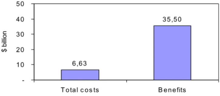
The total costs, adding the supply side of education, opportunity cost, demand and worst forms, is more than six billion dollars PPP. The value obtained for the benefits of education is 35.5 billion dollars PPP (see Graph 10.2).

Graph 10.2.1 – Total cost and total benefit of eliminating child labour

As can be seen in Graph 10.2, the global benefits of the elimination of child labour and the re-direction of these children to education greatly exceed the costs. This result is so strong that it is unlikely that any plausible adjustment to the methodology would reverse it. The principle benefit is, not surprisingly, the economic boost that a country would experience if all children were educat-ed through lower secondary school. The health benefit is far smaller, although this amount is al-most certainly underestimated.

Some sensitivity analysis is shown in table 10.2 considering the elimination of 50% and 75% of the worst forms of child labour instead of 100%, using the Mincerian coefficient in the computa-tion of educacomputa-tion benefits equal to 0.12, 0.13 and 0.14, varying the interest rate to 2%, 4% and 6%, and changing the percentage of GNP per capita to 10% and 20% to convert DALY’s into monetary units. Although some changes are observed, benefits continue being much larger than the costs.

Table 10.2.1 – Sensitivity analysis changing to 50% and 75% the elimination of the worst forms of child labour, using different Mincerian coefficients when calculating education be-nefits, changing the interest rate used to obtain the present values, and changing the percentage of GNP per capita to convert DALY’s into monetary units

Changes Total cost

(in $1000 PPP)

Total benefit (in $1000 PPP)

Worst forms 75% (5%) 6,344,959 35,354,733

Worst forms 50% (5%) 6,021,847 35,354,733

Mincerian coefficient 0.12 (5%) 6,634,297 38,567,195

Mincerian coefficient 0.13 (5%) 6,634,297 41,779,657

Mincerian coefficient 0.14 (5%) 6,634,297 44,992,119

2% 8,788,939 48,635,155

4% 7,260,226 39,175,322

6% 6,083,336 32,022,273

10% GNP per capita (health benefits) 6,634,297 35,381,209

20% GNP per capita (health benefits) 6,634,297 35,425,336

6 ,63

3 5 ,5 0

-10 20 30 40 50

T o ta l c o s ts B e n e fits

$ bi

R

Anderson, Elizabeth. Value in ethics and economics. Cambridge (MA): Harvard Un. Press, 1993.

Basu, Kaushik. Child labor: cause, consequence, and cure, with remarks on international labor stan-dards. Journal of Economic Literature, v. 37, n. 3, p. 1083-1119, 1999.

Basu, Kaushik; Van, P. H. The economics of child labor. The American Economic Review, v. 88, n. 3, p. 412-427, 1998.

Bennell, Paul. Using and abusing rates of return: a critique of the World Bank’s 1995 education sector review. International Journal of Educational Development, v. 16, n. 3, p. 235-48, 1996.

Bloom, D. E.; Canning, D. The health and wealth of nations. Science, 287, 18 February, 2000. Bonnel, R. What makes and economy HIV-resistant? ACT Africa: World Bank, 2000.

Cockburn, John. Income contributions of children in rural Ethiopia. 2001. Unpublished.

Dorman, Peter. Markets and mortality: economics, dangerous work and the value of human life. Cam-bridge: Cambridge University Press, 1996.

Emerson, P.; Souza, A. P. Is there a child labor trap? Intergenerational persistence of child labor in Bra-zil. Economic Development and Cultural Change, v. 51, n. 2, p. 375-398, 2003.

Gallup, John L.; Jeffrey D. Sachs. The economic burden of Malaria. CID Working Paper 52. Cambridge, MA: Center for International Development, Harvard University, 2000.

Glewwe, P. An investigation of the determinants of school progress and academic achievement in Viet-nam. In: Glewwe, Paul; Agrawal, Nisha; Dollar, David (eds.), Economic growth, poverty, and hou-sehold welfare in Vietnam. Washington, DC: World Bank, 2004, p. 467-501.

Grootaert, C.; Patrinos, A. The policy analysis of child labor: a comparative study. Washington, DC: World Bank, 1998, p. 245.

Gunnarsson, V.; Orazem, P. F.; Sanchez, M. A. Child labor and school achievement in Latin América. Wa-shington, DC: World Bank, 2004 (mimeo).

Hammoudi, A. J.; Sachs, J. Economic consequences of health status: a review of the evidence. CID Working Paper N. 30. Harvard University: Center for International Development, 1999.

Heywood, John S. How widespread are sheepskin returns to education in the U.S.? Economics of Edu-cation Review, v. 13, n. 3, p. 227-34, 1994.

Hungerford, Thomas; Solon, Gary. Sheepskin effects in the returns to education. Review of Economics and Statistics, v. 69, n. 1, p. 175-77, 1987.

Jaeger, David A.; Page, Marianne E. Degrees matter: new evidence on sheepskin effects in the returns to education. Review of Economics and Statistics, v. 77, n. 4, p. 733-39, 1996.

Kassouf, A. L. Aspectos sócio-econômicos do trabalho infantil. Min. da Justiça e UNESCO, 2002.

Knight, J. B. Job competition, occupational production functions, and filtering Down. Oxford Economic Papers, 31, p. 187-204, 1979.

Krueger, Alan B.; Lindahl, Mikael. Education for growth: why and for whom? Forthcoming in The Journal of Economic Literature.

Maitra, Pushkar; Ray, Ranjan. The joint estimation of child participation in schooling and employment: comparative evidence from three continents. 2000. Unpublished manuscript.

McCarthy, F. D.; Holger, W.; Yi Wu. The growth costs of malaria. 1999. Unpublished.

Mincer, J. Schooling, experience and earnings. NY: National Bureau of Economic Research, 1974.