ISSN 0104-6632 Printed in Brazil
www.abeq.org.br/bjche
Vol. 29, No. 04, pp. 807 - 820, October - December, 2012
Brazilian Journal
of Chemical
Engineering
OPTIMIZATION AND CONTROL OF A
CONTINUOUS POLYMERIZATION REACTOR
L. A. Alvarez
*and D. Odloak
Department of Chemical Engineering, Polytechnic School, University of São Paulo, Av. Prof. Luciano Gualberto, Trav. 3, 380, CEP: 05508-900, São Paulo - SP, Brazil.
Phone: + (55) (11) 30912237, Fax: + (55) (11) 38132380. E-mail: [email protected]; [email protected]
(Submitted: May 27, 2011 ; Revised: December 9, 2011 ; Accepted: December 30, 2011)
Abstract - This work studies the optimization and control of a styrene polymerization reactor. The proposed strategy deals with the case where, because of market conditions and equipment deterioration, the optimal operating point of the continuous reactor is modified significantly along the operation time and the control system has to search for this optimum point, besides keeping the reactor system stable at any possible point. The approach considered here consists of three layers: the Real Time Optimization (RTO), the Model Predictive Control (MPC) and a Target Calculation (TC) that coordinates the communication between the two other layers and guarantees the stability of the whole structure. The proposed algorithm is simulated with the phenomenological model of a styrene polymerization reactor, which has been widely used as a benchmark for process control. The complete optimization structure for the styrene process including disturbances rejection is developed. The simulation results show the robustness of the proposed strategy and the capability to deal with disturbances while the economic objective is optimized.
Keywords: Polymerization reactor optimization; Model predictive control; Robust operation; Styrene reactor.
INTRODUCTION
The increasing necessity to optimize the operation of chemical reactors is related to the more competitive global market of chemical commodities and specialities. The more competitive a specific market, the more sophisticated the optimization and control strategies of the related industrial plant should be. In the industrial environment, the processes usually operate in a hierarchical structure, where the real time optimization (RTO) and the model predictive control (MPC) are executed in separated stages. The RTO routine determines the operating values of the outputs and inputs that produce the maximum economic profit or the lowest operating costs. In the context of the hierarchical structure, the objective of the MPC controller is to follow the economic targets in the presence of disturbances through the direct manipulation of the process inputs.
uncertainty in the styrene reactor dynamic model. The MPC stage is based on an infinite horizon controller that includes a terminal state constraint (Odloak, 2004), which is extended to uncertain systems. Here, the zone control strategy is also considered (Gonzalez and Odloak, 2009), which consists of mantaining the process outputs inside allowed bounds instead of controlling the process at set-points. The optimization and control structure of the styrene polymerization reactor is tested for the case where the product viscosity and reactor temperature have to be regulated.
The optimization of polymerization processes has been the focus of several works (Kadam et al., 2007; Silva and Oliveira, 2002; Abel and Marquardt, 2003; Asteasuain and Brandolin, 2008). Some of them are dedicated to calculate optimal profiles to achieve the final desired properties in a minimum time. In other works, for example Kadam et al. (2007), the time for polymer grade transition is minimized in order to avoid a considerable amount of off-specification product. In this work, the continuous operation of a styrene polymerization reactor is optimized in a multilayer structure that includes: the RTO layer where an economic objective is considered subject to a rigorous nonlinear model of the polymerization reactor, a control layer where an MPC controller that is robust to a class of model uncertainty, and a target calculation stage that coordinates the communication between the two other layers such that the stability of the control structure is preserved.
In the next section, the styrene polymerization reactor is described; the phenomenological model is presented as well as the linear dynamic models that were obtained. Then, the robust algorithm that integrates the RTO and the MPC controller is presented. Then, the complete real time optimization of the styrene reactor is developed, showing the capability of the proposed strategy to optimize the polymerization process. Finally, in the last section the paper is concluded.
THE STYRENE POLYMERIZATION REACTOR
In this section, we present the main aspects of the reactor system that is studied here and that motivated the development of the control structure that allows the robust operation of the reactor.
Process Description
The polymerization reactor is usually the heart of the polymer production process and its operation may
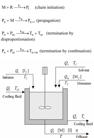
be difficult as it involves exothermic reactions, unknown reaction kinetics and high viscosity. Most styrene polymers are produced through batch or continuous polymerization processes. The present work considers the free-radical bulk and solution styrene polymerization in a jacketed CSTR. As shown in Fig. 1, the CSTR has three feed streams: the pure styrene monomer, the 2,2’-azoisobutyronitrile (AIBN) initiator dissolved in benzene, and the pure benzene solvent. The exit stream contains polymer, un-reacted monomer, initiator, and solvent. The kinetic mechanism used for this homopolymerization process is very general and can be described by the following steps (Jaisinghani and Ray, 1977):
i d
f ,k
I⎯⎯⎯→2R (initiator decomposition)
i
k 1
M+ ⎯⎯→R P (chain initiation)
p
k
n n 1
P +M⎯⎯→P+ (propagation)
td
k
n m n m
P +P ⎯⎯⎯→T +T (termination by disproportionation)
tc
k
n m n m
P +P ⎯⎯→T+ (termination by combination)
Figure 1: Process diagram for the styrene
polymeriza-tion reactor
The two initiation reactions involve the decomposition of initiator I to produce radicals R, which react with the monomer molecules M to initiate new live (radical) polymer chains P1. During
Optimization and Control of a Continuous Polymerization Reactor 809 Pn ( n≥1). The growth of the chains terminates when
the propagating radicals lose their activity through any termination reaction, resulting in dead-polymer chains, Tn (n≥1).
Hidalgo and Brosilow (1990) and Maner et al. (1996) developed a phenomenological model for the styrene reactor. The following considerations lead to the phenomenological model given by Equations (1) to (10):
The lifetime of the polymer radical species is extremely short compared to other system time constants. Then the quasi-steady-state approximation (QSSA) is considered for R and Pn;
The monomer consumption is mainly due to propagation (Biensenberg and Sebastian, 1983), this leads to the Long Chain Assumption (LCA);
Following Hidalgo and Brosilow (1990), the chain transfer reactions to monomer and to solvent are not considered;
Monomer thermal initiation does not occur because this reaction is only significant at temperatures greater than 373K (Biensenberg and Sebastian, 1983). The reactor temperature considered in this work is below this limit;
The overall chain termination rate constant, k , is t composed of both combination, k , and disproportiona-tc tion, k , contributions (Schmidt and Ray, 1981) or td
t tc td
k =k +k . For styrene in solution, experimental results showed that the chain termination occurs solely by combination (Timm and Rachow, 1974). Then, termination by disproportionation is not considered, i.e.
t tc
k =k ;
According to the model presented in Maner et al. (1996), the rate of propagation is much faster than the rate of termination;
The heats of initiation and termination are negligible compared to the heat of polymerization (Hidalgo and Brosilow, 1990).
The styrene reactor model is defined as follows:
i f t
d d[I] (Q [I ] Q [I])
k [I]
dt V
−
= − (1)
m f t
p d[M] (Q [M ] Q [M])
k [M][P]
dt V
−
= − (2)
t f r
p p
c p
dT Q (T T) ( H )
k [M][P]
dt V C
hA
(T T ) C V − −Δ = + ρ − − ρ (3)
c c cf c
c
c c pc c
dT Q (T T ) hA
(T T )
dt V C V
−
= + −
ρ (4)
where,
0,5 i d
t 2f k [I] [P]
k
⎡ ⎤
= ⎢ ⎥
⎣ ⎦ (5)
j
j j
E k A exp ,
T
−
⎛ ⎞
= ⎜ ⎟
⎝ ⎠ j= d, p, t (6)
t i s m
Q =Q +Q +Q (7)
The definition of the parameters and variables involved in the equations above can be found in Tables 1 and 2, respectively. The moment equations for the dead polymer are written as follows:
2
0 t 0
t
dD Q D
0,5k [P]
dt = − V (8)
1 t 1
m p
dD Q D
M k [M][P]
dt = − V (9)
2
p 2
2
M p M 2
t k
dD Q
5M k [M][P] 3M [M] D
dt = + k −V (10)
D0, D1 and D2 represent the zero, the first and the
second order moment of the dead polymer, respectively.
The weight-average molecular weight is obtained as: 2 w m 1 D M M D
= (11)
There are some vendors of instruments to measure efficiently molecular weights by gel permeation chromatography or size-exclusion chromatography, as reported by Richards and Congalidis (2006). However, for online control, it is more common to measure the viscosity as a substitute for the average molecular weights. In this work, it is assumed that an online viscosimeter provides reliable measurements of the intrinsic viscosity η. The following correlation is used to simulate the measurement of the viscosity (Gazi et al., 1996):
0.71 w 0.0012(M )
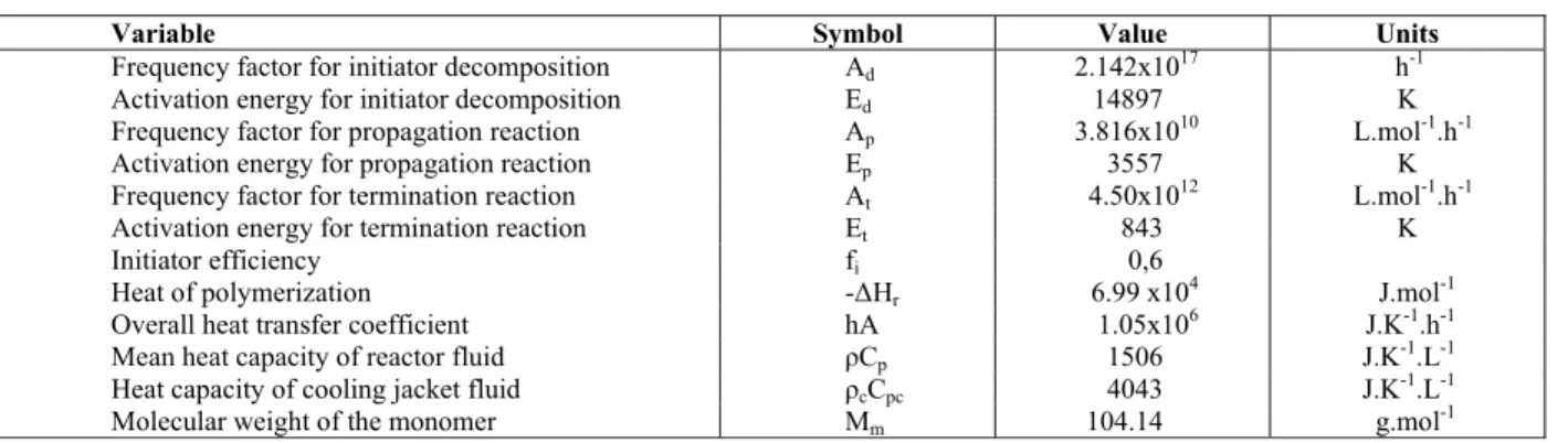
Table 1: Process parameters for the polymerization reactor
Variable Symbol Value Units
Frequency factor for initiator decomposition Ad 2.142x10¹⁷ h-1
Activation energy for initiator decomposition Ed 14897 K
Frequency factor for propagation reaction Ap 3.816x10¹⁰ L.mol-1.h-1
Activation energy for propagation reaction Ep 3557 K
Frequency factor for termination reaction At 4.50x10¹² L.mol-1.h-1
Activation energy for termination reaction Et 843 K
Initiator efficiency fi 0,6
Heat of polymerization -ΔHr 6.99 x10⁴ J.mol-1
Overall heat transfer coefficient hA 1.05x10⁶ J.K-1.h-1 Mean heat capacity of reactor fluid ρCp 1506 J.K-1.L-1
Heat capacity of cooling jacket fluid ρcCpc 4043 J.K-1.L-1
Molecular weight of the monomer Mm 104.14 g.mol-1
Table 2: Steady-state operational condition for the polymerization reactor
Variable Symbol Value Units
Flow rate of initiator Qi 108 L.h-1
Flow rate of solvent Qs 459 L.h-1
Flow rate of monomer Qm 378 L.h-1
Flow rate of cooling jacket fluid Qc 471.6 L.h-1
Reactor volume V 3000 L
Volume of cooling jacket fluid Vc 3312.4 L
Concentration of initiator in feed [If] 0.5888 mol.L-1
Concentration of monomer in feed [Mf] 8.6981 mol.L-1
Temperature of reactor feed Tf 330 K
Inlet temperature of cooling jacket fluid Tcf 295 K
Concentration of initiator in the reactor [I] 6.6832x10⁻² mol.L.-1 Concentration of monomer in the reactor [M] 3.3245 mol.L.-1
Temperature of the reactor T 323.56 K
Temperature of cooling jacket fluid Tc 305.17 K
Molar concentration of dead polymer chains D0 2.7547x10⁻⁴ mol.L-1
Mass concentration of dead polymer chains D1 16.110 g.L-1
The polydispersity index (PD) is a property of the molecular weight distribution of the dead polymer, defined as:
2 0
m 2
1 D D PD M
D
= (13)
The phenomenological model of this styrene reactor was first published in 1990 and, since then, it has been widely used as a benchmark for process control studies (Maner et al., 1996; Gazi et al., 1996; Kendi and Doyle, 1998; Prasad et al., 2002; Asteasuain et al., 2006; Sotomayor et al., 2007). Prasad et al. (2002) implemented a nonlinear MPC strategy for the control of the properties of the polymer. For optimal grade transition, Asteasuain et al (2006) developed a multi-objective optimization that focuses simultaneously on the process design and control parameters. In this work, the aim is to optimize on-line the production rate using a hierarchical structure. The real time optimization is
developed in the upper stage and an intermediary routine recalculates the optimizing targets which are sent to the MPC controller. These stages are tied together and one needs to guarantee the stability of the complete control structure.
Control System and Prediction Models
The purpose of the control system of the styrene reactor is mainly to follow targets for outputs and inputs while mantaining the controlled outputs inside allowed zones. Here, the weight average molecular weight Mw and the reactor temperature T are defined as the controlled outputs. As on-line measurements of Mw are rarely available, the polymer intrinsic viscosity η is used instead. For controlling y1=η and y2=T, the controller
manipulates the initiator flowrate (u1= Qi) and the
liquid flow rate of the cooling jacket (u2= Qc)
Optimization and Control of a Continuous Polymerization Reactor 811 flowrates Qs and Qm are related to Qi by ratio control.
So as to improve the performance of the controller, the ratio between the initiator flow rate Qi and
monomer flow rate Qm is maintained fixed, then:
m
m i
i Q
Q Q
Q
= , (14)
where Qm and Qi are the nominal values of Qm and
Qi, respectively. On the other hand, the solvent
volume fraction should be maintained at 0.6 to avoid
the gel effect (Hidalgo and Brosilow, 1990), then a control law for the solvent flow rate is implemented as:
s m i
Q =1.5Q −Q (15)
The control structure considered for the styrene reactor requires linear models. These models were obtained empirically by step response tests. The nominal model, denoted as MN, used for prediction is the following transfer function model in the Laplace domain is:
66.69 5.9425
(1 5.3474s)(1 2.5274s) (1 7.6525s)(1 3.091s)(1 2.7063s)
G(s)
144.7925 47.5589
(1 6.7599s)(1 1.5797s) (1 7.6173s)(1 2.3968s)
−
⎡ ⎤
⎢ + + + + + ⎥
⎢ ⎥
=
−
⎢ ⎥
⎢ + + + + ⎥
⎣ ⎦
This model relates process inputs and outputs; it was obtained at the nominal operating point presented in the Table 2.
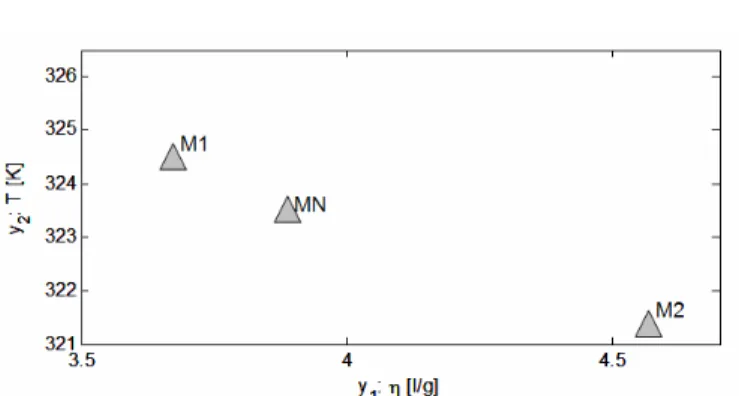
As the aim of this work is to develop an MPC controller that is capable of controlling styrene polymerization reactor at different operating points defined by the RTO stage, two additional models, each one corresponding to a different operating point around the nominal steady-state, were obtained. By modif ying the values of the inputs u1 and u2, from the nominal values u and 1 u , new steady-2 states were obtained and the new linear dynamic models that represent the system around these steady states (Fig. 2) were included in the control problem formulation. The first additional model, denoted by M1, obtained at the steady-state defined by u1=1.1u and u1 2=0.95u , is the following: 2
M1:
61.505 6.9783
(1 5.9946s)(1 2.3723s) (1 8.4587s)(1 2.9801s)(1 2.9801s)
G(s)
166.6494 59.0134
(1 7.542s)(1 1.501s) (1 8.4433s)(1 2.5133s)
−
⎡ ⎤
⎢ + + + + + ⎥
⎢ ⎥
=
−
⎢ ⎥
⎢ + + + + ⎥
⎣ ⎦
Analogously, for the steady-state defined through u1=0.75u and u1 2=1.15u , it 2 was obtained model M2 that is represented as follows:
M2:
90.853 4.2497
(1 6.6137s)(1 3.4171s)(1 3.3297s) (1 6.1175s)(1 3.2567s)(1 2.2792s)
G(s)
116.4704 29.3225
(1 5.6145s)(1 1.5327s) (1 6.1047s)(1 2.152s)
−
⎡ ⎤
⎢ + + + + + + ⎥
⎢ ⎥
=
−
⎢ ⎥
⎢ + + + + ⎥
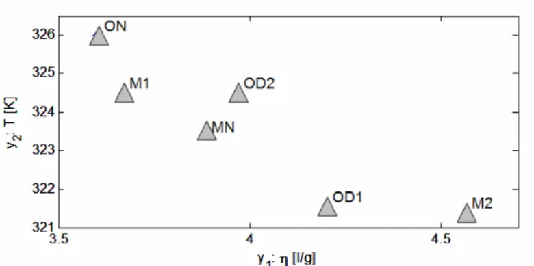
Figure 2: Steady-states values of T and η where the linear models MN, M1 and M2 were obtained.
It is clear that the models defined above do not have the same gain or the same time constants as the nominal model. Then the effect on the output prediction is significant. So, there is motivation to consider a control structure where stability and performance is preserved despite the operation at quite different steady-states.
ROBUST CONTROL STRATEGY
The rigorous steady-state version of the model defined through Equations (1) to (13) is used to represent the true reactor at steady-state in the optimization problem that defines the RTO stage of the structure represented in Fig. 3. The MPC stage is based on a robust linear MPC that is presented next.
System Representation
Although the available dynamic models of the styrene reactor are in the transfer function form, the MPC considered here is based on a state space model as is usual in modern MPC packages. To describe this model, let us consider a system with nu inputs and ny outputs, and assume that the poles that relate the input ui to the output yj are non-repeated. A state
space model that is suitable to the implementation of an offset free MPC can be represented in the following form (Odloak, 2004):
s s 0
ny
d d d
I 0
x (k 1) x (k) D
u(k) 0 F
x (k 1) x (k) D
⎡ + ⎤ ⎡ ⎤⎡ ⎤ ⎡ ⎤
= + Δ
⎢ ⎥ ⎢ ⎥⎢ ⎥ ⎢ ⎥
+
⎢ ⎥ ⎣ ⎦⎢ ⎥ ⎢ ⎥
⎣ ⎦ ⎣ ⎦ ⎣ ⎦ (16)
s
ny d
x (k) y(k) I
x (k)
⎡ ⎤
⎡ ⎤
=⎣ Ψ ⎢⎦ ⎥
⎢ ⎥
⎣ ⎦
where
T s
1 ny
x = ⎣⎡x " x ⎤⎦ , xs∈\ny,
T d
ny 1 ny 2 ny nd
x = ⎣⎡x + x + " x + ⎦⎤ , xd∈^nd,
.
nd nd
F∈^ , u(k)Δ =u(k)−u(k 1)− , Ψ ∈\ny nd×
The input in the model defined in Eq. (16) is u(k)
Δ , which means that the output integrates the input. In this model, the state vector is split in two parts: xs that corresponds to the integrating poles produced by the incremental form of the model, and xd that corresponds to the system modes. The state component xs corresponds to y( |k)∞ that is the predicted output at steady-state. For stable systems, it is easy to show that when the system approaches the steady-state, component xd tends to zero. F is a diagonal matrix with components corresponding to the poles of the system. The system has nd stable poles.
In the model defined in Eq. (16), model uncertainty is related to the uncertainty in matrices F, D0 and Dd, as discussed in Alvarez and Odloak (2010). Then, suppose one defines the set of possible plants as Ω = θ θ
{
1, 2,...θL}
, where each θi corresponds to a particular plant θ =i(
F , D , Di 0i di)
,i=1, 2,...L. The true model of the process system is unknown, but one can assume that it can be represented as θ =r
(
F , D , Dr 0r dr)
, where(
)
L(
)
0 d 0 d
r r i i i
i 1
D , D D , D ,
=
=
∑
λL
i i
i 1
1, 0
=
λ = λ ≥
∑
andr j 1,2...L
Optimization and Control of a Continuous Polymerization Reactor 813 0
r
D and D lies in a convex polytope defined by L dr vertices (Kothare et al., 1996), while F belongs to a r finite set of possible dynamics (Badgwell, 1997). In this way, uncertainty in the gain matrices D , D is defined 0r dr as polytopic (Kothare et al., 1996) while the uncertainty in F is assumed to be of the multi-plant type (Badgwell, 1997). Assume also that there is a most likely plant that also lies in Ω and is denoted by θn.
Badgwell (1997) developed a robust linear quadratic regulator for stable systems with the multi- plant uncertainty. Later, Odloak (2004) extended the method of Badgwell to the output tracking of stable systems considering the same kind of model uncertainty. These strategies include a constraint to each of the models lying in Ω that prevents the increase of the true plant cost function at sucessive time steps. Gonzalez and Odloak (2009) proposed a stable MPC controller where the outputs are controlled by zones instead of at fixed set-points. In the method followed here, the approach of Odloak (2004) and the zone control strategy are applied to the multiple stage structure represented in Fig. 3, as described in the following section.
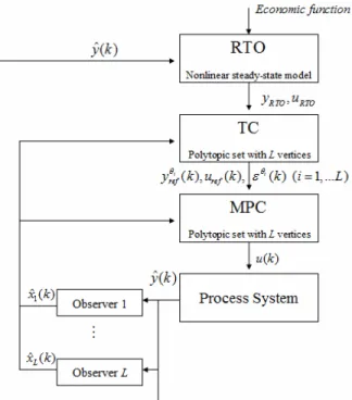
Control Structure
The control structure considered in this work is represented in Fig. 3. In this structure, the RTO layer is dedicated to the calculation of the desired targets
RTO
u and yRTO, for the input and output variables
of the styrene reactor. This layer is commonly based on the rigorous stationary model and takes into account the process measurements and the economic parameters. The second layer is the target calculation (TC) algorithm that, at each time step, re-computes feasible steady-state operating points assuming that the RTO routine produces piecewise constant optimizing references for inputs and outputs. As discussed in Ying and Joseph (1999), the main purpose of the target calculation routine is to compute achievable set-points for the MPC controller. The targets i
ref
yθ (k), i=1,...L and uref(k) are obtained through the solution of an optimization problem based on the nominal linear static model of the process system. Then, the solution of the TC stage is sent to the MPC controller, which is devoted to guide some of the reactor inputs and/or outputs to the desired values given by the TC stage, while keeping the other reactor controlled outputs within specified zones.
In terms of the frequency at which each stage is computed, the RTO stage is solved at a much slower pace than the lower level control stages. This allows a dynamic decoupling between the RTO stage and the TC/MPC stages. Thus, one observes that the stability of the styrene reactor in closed loop with the structure represented in Fig. 3 depends only on the interaction between the TC and MPC stages. Consequently, the target calculation stage, that coordinates the interaction between the RTO and MPC stages, has to be designed in such a way that stability of the control structure is preserved.
On the other hand, note that from the control structure depicted in Fig. 3, there is one state observer per each model, and the observer corresponding to the true model θr is based on the true model matrices and will indicate the true state for the undisturbed system. In this case, at each sampling step, the corrected state is sent to the TC and MPC stages to calculate the next control action according to the algorithm that is described in the following section.
RTO Problem
The RTO layer deals with the economic optimization. In this case, the maximization of the production rate is considered as the economic objective. The production rate is defined as the product of the total flowrate Qt and the first order
moment D1, this product represents the total weight
of dead polymer produced per time unit. The RTO routine solves the following economic optimization problem:
RTO RTO
t 1
y max,u ,x Q D (17)
subject to:
RTO RTO
h(y , u , x)=0 (18)
1.49≤PD≤1.51 (19)
min RTO max
u ≤u ≤u (20)
min RTO max
y ≤y ≤y (21)
where,
RTO RTO
h(y , u , x) represents the nonlinear steady-state model and x is the vector of states of the
phenome-nological model, x=
[
[I],[M],T,T , D , D , Dc 0 1 2]
T. Observe that D1 is one of the states of thephenomenological model in Eq. (8). The problem includes a bound constraint on the polydispersity PD, which depends on three states of the process model. This property is a strong indicator of the polymer quality. In this case, it is desired to maintain the polydispersity around the nominal value of 1.5. Note that this RTO problem is a nonlinear programming (NLP) since the constraints in Eqs. (18) and (19) are nonlinear. Here, it is assumed that the disturbances are measured and the optimization problem is updated at each sample time; both the process model state D1 in Eq. (17) and the model constraints in Eqs.
(18) and (19) are then modified as the disturbances are introduced. From the solution of this problem, only yRTO and uRTO are passed to the TC stage.
Robust Algorithm for the TC and MPC Stages
In this section, the robust structure, which is defined by the TC and the MPC optimization algorithms, is described. Let us denote the cost function for the TC stage at time k by JTCk . For each model i, i=1,...L the objective function associated with model i is defined as follows:
i
y i
u i
2 TC
k i ref RTO
W
2 2
ref RTO
W S
J ( ) y (k) y
u (k) u (k)
θ
θ
θ = −
+ − + ε
(22)
where the weighting matrices W , Wy u and
i
S (i=1...L) are positive definite.
Then, at the TC stage, the following optimization problem is solved (Alvarez and Odloak, 2010):
i
i ref i i
ref
L
2 TC
n
S
y (k),u (k), (k) i 1
i 1,...L i n
min J ( ) (k)
θ θ
θ
ε =
= ≠
θ +
∑
εk
subject to:
ref
u (k)∈U,
{
max ref max}
ref
max min ref
m u u (k) u(k 1) m u U u (k)
u u (k) u
− Δ ≤ − − ≤ Δ
= ≤ ≤ (23)
[
]
i s 0
i ref
ref
yθ (k)−x (k)=D ( ) uθ (k)−u(k 1) ,−
(24) i=1,...L
i
i i
min ref max
y + εθ(k)≤yθ (k)≤y + εθ(k), (25) i=1,...L
TC TC
i i
Jk ( )θ ≤Jk ( ),θ i=1,...L (26)
In this problem, JTCk ( )θi is the cost associated with the solution of the same problem at the previous sampling step that is defined as
{
i * i*}
ref ref
yθ (k), u (k 1),− εθ (k 1) ,− where i
ref yθ (k) is
Optimization and Control of a Continuous Polymerization Reactor 815
(
)
i s 0
i ref
0 *
i ref
y (k) x (k) D ( ) u(k 1)
D ( ) u (k 1) u(k 2)
θ − + θ Δ − =
θ − − −
(27)
The TC optimization problem minimizes the cost for the nominal model θn subject to constraints related to models θ1,...θL. The equality constraints Eq. (24) correspond to the steady-state linear models relating the predicted output with the desired steady-state, u(k 1)− is the control action applied to the real
system at the previous time step, εθi(k) are slack
variables that soften the bound constraints associated with each i
ref
yθ (k) and allow these variables to take values outside the output control zone, and m is the control horizon of the MPC controller considered in the MPC stage in Fig. 3 The constraints represented in Eq. (24) force the decrease of the cost function
TC
Jk for all the L models. Note that, if at time step k a disturbance enters the system the solution
{
i* * i*}
ref ref
yθ (k 1), u− (k 1),− εθ (k 1)− that is inherited
from time k 1− may be unfeasible. By replacing
i*
ref
yθ (k 1)− with i
ref
yθ (k) computed through Equation
(27), where the actual state x (k) is used, the s optimization problem of the TC stage is always feasible.
The optimal solution of the TC stage
{
i * * i*}
ref ref
yθ (k), u (k),εθ (k) is then sent to the MPC
stage, where a constrained infinite horizon MPC controller is implemented. The optimization problem, which has the same sampling period as the TC stage, is defined as follows:
i
i i i
k sp L 2 MPC n P u ,y (k), (k)
i 1
i 1,...L i n
min J ( ) (k)
θ θ
θ
Δ δ =
= ≠
θ +
∑
δk
subject to:
u(k j k) V,
Δ + ∈
max max
min j
max i 0
u u(k j) u u u(k 1)
V u(k j) u(k i) u
u(k j) 0, j m
=
−Δ ≤ Δ + ≤ Δ
⎧ ⎫
⎪ ≤ − ⎪
⎪ ⎪
⎪ ⎪
= Δ⎨ + + Δ + ≤ ⎬
⎪ ⎪
⎪ ⎪
Δ + = ≥
⎪ ⎪
⎩ ⎭
∑
(28)i i
s 0
i k sp
x (k) D ( ) u y (k) (k) 0,
i 1,...L
θ θ
+ θ Δ − − δ =
=
(29)
0 0 0
m D = ⎣⎡D ... D ⎤⎦
i i
i *
sp ref
y (k)θ =yθ (k)− δθ(k), i=1,...L (30)
i(k) i*(k), i 1,...L
θ θ
δ = ε = (31)
i
min sp max
y ≤y (k)θ ≤y , i=1,...L (32)
*
k ref
u(k 1)− + Δ −I u u (k)=0 (33)
[
nu nu]
m I= I ... I
, Inu is the identity matrix with
dimension nu
MPC MPC
i i
Jk ( )θ ≤Jk ( ),θ i=1,...L (34)
In this problem, the infinite horizon cost MPC
k i
J ( )θ is defined as:
i i i
y u i i MPC k i 2 sp Q 2 * ref Q
j 0 2
R
2 P J ( )
ˆy (k j k) y (k) (k)
u(k j k) u (k)
u(k j k)
(k)
θ θ θ
∞
=
θ
θ =
⎡ + − − δ ⎤
⎢ ⎥
⎢ ⎥
+ + −
⎢ ⎥
⎢ ⎥
⎢+ Δ + ⎥
⎢ ⎥
⎣ ⎦
+ δ
∑
(35)i=1,...L
where the weight matrices Q , Q , Ry u and
i
P (i=1...L) are positive definite.
that the terminal constraints in Eq. (29) are always feasible and the cost functions JMPCk ( ), iθi =1,...L are bounded. Constraints in Eqs. (30) and (31) are applied only to those outputs that have optimizing targets, while constraint in Eq. (32) is written for the outputs without optimizing targets. Also, the equality of the slacks of the TC and MPC stage defined in Eq. (31) guarantee that the solution of the MPC problem will not disrupt the convergence of the cost function of the TC stage. The set of constraints in Eqs. (25) to (27) assures that the solution of the MPC problem is consistent with the solution of the TC stage problem. Constraint in Eq. (33) is related to the input targets, so it is only written for those inputs that have optimizing targets. The constraint represented in Eq. (34) involves the cost JMPCk ( )θi , which is calculated with the solution
{
i i}
k sp
u , y (k),θ θ(k)
Δ δ , where:
T
* T * T
k
u ⎡ u (k k 1) ... u (k m 2 k 1) 0⎤
Δ = Δ⎣ − Δ + − − ⎦
i i*
sp sp
y (k)θ =yθ (k 1),− i=1,...L
and δy,i(k) is such that
i i
s 0
i k sp sp
x (k)+D ( ) u θ Δ − y (k)θ − δθ(k)=0, i=1,...L
Observe that the set
{
i i}
k sp
u , y (k),θ θ(k)
Δ δ is a
feasible solution inherited from the time instant k 1− based on the present state x (k) . s
This control structure guarantees robust stability (Alvarez and Odloak, 2010). If the RTO targets are reachable, the process variables converge to the desired targets while the cost functions correspond-ing to the TC and MPC stages converge to zero for each model i (i=1,…L) and consequently for the true model. Otherwise, the cost function of the TC stage converges to a point where the distance between
(
yRTO, uRTO)
and(
yrefn, urefn)
θ θ
is minimized.
In the next section, the behavior of this robust structure applied to the styrene polymerization reactor is tested.
SIMULATION RESULTS
For this simulation, targets for the output y2 and
input u1 were defined. Two disturbances affect the
process during 400 hours of simulation. This controller considers the three linear models for prediction. The simulation conditions are the following: The constraint values: umax = [0.070 ; 0.25] ;
umin = [0.015 ; 0.08] ; Δumax = [0.1 ; 0.1]; ymax = [4.15 ;
326] ; ymin = [3.5 ; 321]. The initial conditions: u0 =
[0.03; 0.131] ; y0 = [3.9;323.5]. The following tuning
parameters are considered: Cy = [0 1] ; Cu = [5 0] ;
Cε = 1e5×[1 1]; m = 3; Qy = [1 1] ; Qu = [200 0] ;
R = [10 10] ; Sy = 1e5×[1 1].
First, at t=0 the process starts at a non-optimal steady-state and the controller tries to bring the process to the optimal target calculated by the RTO routine. Fig. 4 shows the process outputs (black line), RTO targets (green discontinuous line) and the targets calculated in the TC stage (blue discontinuous line). The output target for y2 and
output y2 both reach the RTO target, which is at the
upper bound of the zone, while output y1 reaches a
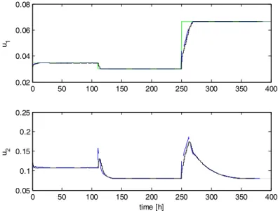
different steady-state value inside its control zone. As can be seen in Fig. 5, the input u1 also reaches
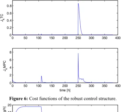
the RTO target. By observing Fig. 7, one can see that the production rate is increased and so the complete structure is efficient enough to maximize the production. Fig. 6 shows that, at the beginning, the cost function of the TC stage converges to zero and then in the MPC stage also converges, which means that the process variables followed the desired objectives.
The first disturbance occurs at time t=110h, and corresponds to a sudden decrease of 4 °C in the temperature of the feed. This disturbance has a large effect on y1, which is the viscosity of the product and
also, as expected, on y2, the reactor temperature.
Notice that both outputs are pushed to outside their zones and the control system brings them back to inside the zones. This disturbance moves the optimal steady-state and the RTO calculates new target values for both y2 and u1. Figure 4 shows that the
new target for the output y2 corresponds to a lower
temperature and the control system is able to bring this output to its target. As can be seen in Fig. 5, the RTO sends a new target for u1 which is easily
reached, while the input u2 decreases. This means
Optimization and Control of a Continuous Polymerization Reactor 817 After 250 hours of simulation, when the process
had reached the steady-state, a second disturbance was introduced in the reactor. There was an abrupt decrease from 0.59 to 0.54 mol/l in the initiator feed concentration. In this case, the RTO computes a different value for the targets of u1 and y2, both
variables are able to reach the targets. Fig. 4 shows that this disturbance pushed the viscosity (y1) to
outside the zone and the TC target for y1 decreases to
the lower bound of the zone, then this target increases while the viscosity is recovered reaching
the target. Note that at first, the controller was bringing the TC targets to a smaller value of y1 and a
larger value of u2 to adjust the process to the new
RTO targets. However, when the target for y1
reached its lower bound, the controller had to readjust these TC targets to feasible values changing the direction of u2. In this case, the process is moved
to a new optimal steady-state, as shown in Fig. 5. This disturbance drives the process to an optimal production rate, which is larger than the last one, as can be seen in Fig. 7.
0 50 100 150 200 250 300 350 400
3.4 3.6 3.8 4 4.2 4.4
y1
0 50 100 150 200 250 300 350 400
320 322 324 326 328
time [h]
y2
Figure 4: Process outputs. Red dashed line: Output bounds.
Blue dashed line: calculated targets. Green dashed line: RTO targets. Solid line: Process outputs.
0 50 100 150 200 250 300 350 400
0.02 0.04 0.06 0.08
u1
0 50 100 150 200 250 300 350 400
0.05 0.1 0.15 0.2 0.25
time [h]
u2
Figure 5: Process inputs. Blue dashed line: calculated input
0 50 100 150 200 250 300 350 400 0
0.2 0.4 0.6 0.8
Jk
TC
0 50 100 150 200 250 300 350 400
0 2 4 6 8
Jk
MP
C
time [h]
Figure 6: Cost functions of the robust control structure.
0 50 100 150 200 250 300 350 400
10 12 14 16 18 20
P
ro
d
u
cti
o
n
ra
te
[K
g
/h
]
time [h]
Figure 7: Production rate of the process.
The polydispersity is a property that indicates the distribution of the polymer chain size in the product. Additionally, the intrinsic viscosity η measures indirectly the average molecular weight of the polymer produced (Gazi et al., 1996). Both molecular weight and polydispersity are strong indicators of polymer quality. Fig. 8 shows the simulation results for the polydispersity, it can be seen that this property remains near its nominal value of 1.5, respecting the limits imposed by the RTO problem even when disturbances affect the process.
Finally, Fig. 9 shows the optimal steady-states reached during the RTO simulation as a function of
the outputs. The first steady-state (ON) corresponds to the optimal nominal conditions and, although it is close to the M1 steady-state, it is far from the remaining MN and M2 steady-states. The first disturbance brought the process to the optimal steady-state OD1, which is near the MN and M2. Then, the second disturbance moved the optimal steady-state to a point denoted by OD2, for this point, the MN is the closest steady-state. This demonstrates that the proposed robust RTO/TC/MPC strategy can deal with disturbances that drive the process to different operating points and result in different optimum points.
0 50 100 150 200 250 300 350 400
1.496 1.498 1.5 1.502 1.504 1.506
P
ol
y
di
s
p
er
s
it
y
time [h]
1.496 1.498 1.5 1.502 1.504 1.506
P
o
lyd
isp
e
rsi
ty
0 50 100 150 200 250 300 350 400
time [h]
0 50 100 150 200 250 300 350 400
1.496 1.498 1.5 1.502 1.504 1.506
P
ol
y
di
s
p
er
s
it
y
time [h]
1.496 1.498 1.5 1.502 1.504 1.506
P
o
lyd
isp
e
rsi
ty
0 50 100 150 200 250 300 350 400
time [h]
Optimization and Control of a Continuous Polymerization Reactor 819
Figure 9: Steady-states values of T and η corresponding to the
optimum at the nominal operating condition (ON), after the first disturbance (OD1), after the second disturbance (OD2) and where linear models MN, M1 and M2 were obtained
CONCLUSIONS
In this work the robust control and optimization of a styrene polymerization reactor was studied. The control structure includes a TC stage between the RTO and MPC routines which recalculates feasible targets for the MPC. Model uncertainty is considered in the TC and MPC stages of the control structure. For linear systems, the strategy assures stability in a polytopic region where the model uncertainty was defined. The resultant scheme is robust as the algorithm guarantees convergence to the desired targets for the uncertain model. The approach was simulated in the styrene polymerization reactor, which is a nonlinear system. Multiple linear dynamic models were obtained around different operating points, and considered as the vertices of a polytopic region where the real system operates. The simulation results of the complete RTO structure showed that the approach is capable of maximizing the production rate in the presence of disturbances, preserving the polymer quality and satisfying the allowed limits for the controlled outputs.
ACKNOWLEDGEMENTS
Authors are grateful to FAPESP for the financial support under grant 2008/57511-9.
REFERENCES
Abel, O. and Marquardt, W., Scenario-integrated on-line optimisation of batch reactors. J. Proc. Cont., 13, p. 703-715 (2003).
Alvarez, L. and Odloak, D., Robust integration of real time optimization with linear model predictive control. Comp. Chem. Eng., 34, p. 1937-1944 (2010).
Asteasuain, M., Bandoni, A., Sarmoria, C., Brandolin, A., Simultaneous process and control system design for grade transition in styrene polymerize-tion. Chem. Eng. Sci., 61, p. 3362-3378 (2006). Asteasuain, M. and Brandolin, A., Modeling and
optimization of a high-pressure ethylene polymerization reactor using gPROMS. Comp. Chem. Eng., 32, p. 396-408 (2008).
Badgwell, T., Robust model predictive control of stable linear systems. Int. J. Control, 68 (4), p. 797-818 (1997).
Biensenberg, J. and Sebastian, D., Principles of Polymerization Engineering. Wiley, New York (1983).
Gazi, E., Seider, W., Ungar, L., Verification of controllers in the presence of uncertainty: Application to styrene polymerization. Ind. Eng. Chem. Res., 35, p. 2277-2287 (1996).
González, A., Marchetti, J., Odloak, D., Extended robust model predictive control of integrating systems. AIChE J., 53, (7), p. 1758-1769 (2007). González, A., Odloak, D., A stable model predictive
control with zone control. J. Proc. Cont., 19, p. 110-122 (2009).
Hidalgo, P., Brosilow, C., Nonlinear model predictive control of styrene polymerization at unstable operating points. Comp. Chem. Eng., 14, p. 481-494 (1990).
Kadam, J., Marquardt, W., Srinivasan, B. and Bonvin, D., Optimal grade transition in industrial polymerization processes via NCO tracking. AIChE J., 53, p. 627-639 (2007).
Kendi, T., Doyle III, F., Nonlinear internal model control for systems with measured disturbances and input constraints. Ind. Eng. Chem. Res., 37, p. 489-505 (1998).
Kothare, M., Balakrishnan, V., Morari, M., Robust constrained model predictive control using linear matrix inequalities. Automatica, 32, (80), p. 1361-1379 (1996).
Maner, B., Doyle III, F., Ogunnaike, B., Pearson, R., Nonlinear model predictive control of a simulated multivariable polymerization reactor using second-order Volterra models. Automatica, 32, (9), p. 1285-1301 (1996).
Odloak, D., Extended robust model predictive control. AIChE J., 50 (8), p. 1824-1836 (2004).
Prasad, V., Schley, M., Russo, L., Bequette, B., Product property and production rate control of styrene polymerization. J. Process Control, 12, p. 353-372 (2002).
Richards, J. and Congalidis, J., Measurement and control of polymerization reactors. Comp. Chem. Eng., 30, p. 1447-1463 (2006).
Schmidt, A. and Ray, W., The dynamic behavior of continuous polymerization reactors–I Isothermal solution polymerization in a CSTR. Chem. Eng. Sci., 36, p. 1401-1410 (1981).
Silva, D. and Oliveira, N., Optimization and nonlinear model predictive control of batch polymerization systems. Comp. Chem. Eng., 26, p. 649-658 (2002).
Sotomayor, O., Odloak, D., Giudici, R., Diagnosis of abnormal situations in a continuous solution polymerization reactor. Macromol. Theory Simul., 16, p. 247-261 (2007).
Timm, D. and Rachow, J., Description of polymeri-zation dynamics by using population density. H. M., Hulburt, Chemical Reaction Engineering–II, Advances in Chemistry Series 133. Am. Chem. Soc., p. 122-136 (1974).