ISSN 0104-6632 Printed in Brazil
Vol. 21, No. 03, pp. 435 - 447, July - September 2004
Brazilian Journal
of Chemical
Engineering
A MATHEMATICAL MODEL FOR ISOTHERMAL
HEAP AND COLUMN LEACHING
L.R.P. de Andrade Lima
*Department of Chemical Engineering, McGill University, 3610 University Street, Montreal, Quebec, Canada H3A 2B2
Tel +(1) 514-398 4491, Fax +(1) 514-398 6678 E-mail: [email protected]
*On leave from Department of Materials Science and Technology, Federal University of Bahia,
Rua Aristides Novis 2, Salvador - BA, Brazil, 40210-630.
(Received: July 13, 2003 ; Accepted: April 19, 2004)
Abstract - Leaching occurs in metals recovery, in contaminated soil washing, and in many natural processes, such as fertilizer dissolution and rock weathering. This paper presents a model developed to simulate the transient evolution of the dissolved chemical species in the heap and column isothermal leaching processes. In this model, the solid bed is numerically divided into plane layers; the recovery of the chemical species, the enrichment of the pregnant leach solution, and the residual concentration of the leaching agent are calculated by interactions among the layers. The solution flow in the solid bed is assumed as unidirectional without dispersion, and the solid-fluid reaction is described by a diffusive control model that is integrated analytically for each time step. The data set used in the model include physical-chemical, geometrical, and operational variables, such as: leachable chemical species content, leaching agent flow rate and concentration, particles size distribution, solution residence time in the solid bed, and solid bed length, weight and irrigated area. The results for two case studies, namely, an industrial gold heap leaching and a pilot column copper acid leaching, showed that the model successful predict the general features of the process time evolution.
Keywords: leaching processes, solid-fluid reaction, extractive metallurgy.
INTRODUCTION
Industrial processes based in the selective dissolution of chemical species have been used for many years as an effective method to recovery metals such as gold, silver, copper, zinc, nickel, cobalt, and uranium, and salts as potassium nitrate from ores and concentrates. Leaching processes have also been used in a broad class of remediation techniques, generally called soil washing, used to clean up soils and other solids contaminated by inorganic and organic compounds; fertilizer dissolution in soils, acid mine drainage in sulphidic mineral waste, heavy metals dissolution from metallurgical slags and mineral or concrete weathering are other processes where leaching occurs.
In industrial applications, the leaching process
can take place in tanks, vats, heaps, dumps or columns. In conventional heap leaching process, the solid particles (crashed ore or aggregated mineral concentrate) are disposed on a sloped impervious surface, and on the top a leaching solution (sulfuric or hydrochloric acid, cyanide, or water) is sprayed or trickled to gradually percolate the solid bed down to the impervious base where the pregnant solution is drained and sent to a recovery step (by precipitation or by adsorption on activated carbon). Similarly, in the column leaching process, the solid particles are carefully disposed inside a cylindrical column and on the top a leaching solution is trickled to gradually percolate the solid bed to the bottom where the pregnant solution is directed to the recovery step.
material, experiments in batch, small column or small heap are often performed and the results are extrapolate by using rule of thumb to represent the industrial heaps or dumps. These tests provide information about the leaching agent consumption, the maximum recovery of the chemical species, and the rate of recovery; however, the scale-up to industrial heaps or large columns are not directly possible due to the difficult to reproduce the physical characteristics; moreover, these experiments are time and cost demanding, which stimulated the development of mathematical models, particularly to describe the acid leaching of oxidized and sulfide copper ores, the gold cyanidation, the sulphidic oxidation in overburden dumps, and the laterite acid leaching.
The available heap, dump and column leaching phenomenological models are based on the mass balance of the reactants in the solid bed and particles, on specific kinetic models to describe the solid-liquid reactions, and in some cases, on the energy and the momentum balances. Here are mentioned only a few more relevant or recent papers, but an extensive literature survey can be found in de Andrade Lima (1992).
A detailed phenomenological model to dump leaching process was first developed by Cathles and Apps (1975) and Cathles and Schlitt (1980) to describe the leaching of a copper sulfide waste; in this model the conservation of mass, energy and momentum equations applied to bed and solid particles were used. Next, Davis and Ritchie (1986) and Davis et al. (1986) developed a model to the pyritic oxidation in overburden dumps using the conservation of mass to the bed and the solid particles. After, Pantelis and Ritchie (1991, 1992) and Pantelis et al. (2002) also studied the oxidation of sulphidic waste rock dumps taking into account a detailed conservation of energy and momentum equations in the bed. Dixon and Hendrix (1993) assuming solution plug flow through the bed, diffusion of the reagents into the particles of the ore, and a first order kinetic model described the gold heap cyanidation; this model was validated with column experimental results for a synthetic mineral association submitted to cyanidation. After, Sánchez-Chacón and Lapidus (1997) presented a similar approach to describe the gold heap cyanidation process using a more detailed kinetic model and changed a boundary condition from the original formulation. Recently, Petersen and Petrie (2000) applied Dixon’s model to describe a
ferro-chromium slag deposits leachate potential; more recently, Petersen and Dixon (2002) extended the original Dixon’s model adding heat conservation, gas flow, bacterial growth kinetics and complex reactions schemes that could describe the thermophilic copper sulfide bio-heap leaching. On the other hand, a most comprehensive model, but also useful and rigorous to isothermal problems as the case of conventional acid leaching of oxidized copper ores and cyanidation of gold ores, was first introduced by Roman et al. (1974). In this model, an algorithm is used to describe the liquid plug flow inside the heap and the shrinking core model under diffusive control is used to describe the ore/acid reaction. This heap model was originally evaluated using column experiments and, since then has been used to describe many industrial and pilot heaps and columns of oxidized copper ore acid leaching (Roman et al.,1999). Later, Box and Prosser (1986) proposed a generalization of Roman’s model by taking into account the simultaneous interactions of several mineral particles and reagent solutions, as well as the leaching products that eventually may be part of these reacting systems. In this case, the shrinking core model under diffusive control was used to describe many ore particles/leaching solution reactions, and the Roman’s algorithm was used to describe the liquid plug flow in the ore bed. After, Prosser (1989) applied this model to describe both columns and industrial heaps in the case of gold ore/cyanide systems associated with other leached metals, obtained promising results.
The main objective of this paper is develop a comprehensive model to describe the isothermal heap and column leaching process that can be useful to routinely design studies, such as heap or column leaching and washing sequences, as well as, pregnant solution blend from heaps at different reaction stages. In this paper, some ideas from the models developed by Roman et al. (1974) and Box and Prosser (1983) were improved and others modified; for instance, here the solid-liquid kinetic equation is integrated analytically instead to the conventional numerical integration, the model parameters evaluation are performed directly from experimental data, and in the flow calculation, the particles bed is divided in planar element to conveniently describe the heap or column geometric shape instead to columnar elements.
studies: an industrial gold heap leaching and a pilot column copper leaching; finally, the fourth section presents the conclusions.
THE MATHEMATICAL MODEL
The heap and column leaching process are a kind of trickle-bed reactor where the solid particles can react with both phases: air and dissolved leaching agent (de Andrade Lima, 1992). The minimal requirement for a reliable mathematical description of this process has to take into account the fluid flow throughout the porous ore bed and the solid-liquid reaction that takes place in the ore particles, which are the main phenomena that happened in this process. As mentioned in the previous section, in this paper some ideas from the models developed by Roman et al. (1974) and Box and Prosser (1983) were used and modified; those models assume that the axial and radial dispersions of the liquid flow throughout the solid bed negligible, the solid/leaching agent reaction is controlled by diffusion of the reactant species through the solid particles, the average residence time of the solution inside the heap does not change with time or position, and the amount of leachable species, the size of the solid particles are homogeneous distributed in the heap, and the temperature is constant. In the present model these assumptions also hold; however, instead of dividing the solid particles bed in columnar elements to conveniently describe the heap or column geometric shape, planar elements are used; in addition, instead of using a numerical method to integrate the solid-liquid kinetic model, an analytical integration is used, which gives less dependence of the number of numerical elements used in the calculations and reduces the simulation time. Finally, instead of trying to evaluate the model parameters from first principles, which are unrealistic in the case of heterogeneous materials as ores and concentrates, here these parameters are estimated by fitting the model results to real data.
Liquid Flow Model
In the present model, the heap is represented as a regular solid, such as a parallelepiped or a cylinder, which are divided in nl layers of equal thickness; the pregnant and leach solutions that flow through the several layers of the heap are retained in each one for a duration of time equal to 'W W/nl. Since the average residence time of such solution, in each layer, is constant, the liquid hold-up of the heap is related with the operational and geometric heap or column characteristics as follows:
HB HBHB HB
ı İ IJ Q H S (1)
where HHB is the heap porosity, VHB is the heap
saturation, W is the average residence time of the solution in the bed of the heap, Q is the rate of irrigation in the heap, HHB is the average heap height or bed length, and SHB is the average heap top
surface.
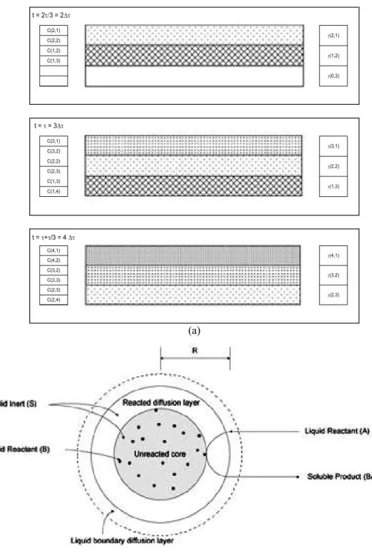
The solution flow in the bed is taken into account by using an algorithm, which progress for a three-layer heap is schematic summarized in Fig. 1a. In this algorithm, first the leaching solution enters on the top of the heap in the first layer (j=1), where it remains for an amount of time 'W=W/3. Later, the solution is transferred to the next layer (j=2) and stay there for the same time, and from this to the next layer until it reaches the last one (j=3). During the time that the liquid solution remains in each layer, the kinetic equation is solved for each chemical species (m) contained in each size-fraction (i) by taking into account the solid residual specie contents (J) and its concentration in the solution (CA and CB). After that, the residual content of the species in the solid particles and in the solution is updated. The solution increments do not mix one to another (plug flow assumption), so the heap bed has in a given simulation time (t), residual solids of concentration J(t,j) and increments of solution with concentration C(t,j) in different layers (j=1, 2, 3 ) with different reaction times (t=0, 1, 2, 3, 4).
C(1,1)
C(1,2) J(1,1)
J(0,2)
J(0,3)
C(2,1)
C(2,2) J(2,1)
J(1,2)
J(0,3) C(1,2)
C(1,3)
t = 2W3 = 2'W
C(3,1)
C(3,2) J(3,1)
J(2,2)
J(1,3) C(2,2)
C(2,3) C(1,3) C(1,4)
t = W = 3'W
C(4,1) C(4,2)
J(4,1)
J(3,2)
J(2,3) C(3,2)
C(3,3) C(2,3) C(2,4)
t = W+W/3 = 4 'W
(a)
Liquid Reactant (A) R
Soluble Product (BA)
Liquid boundary diffusion layer Reacted diffusion layer
Unreacted core
(b)
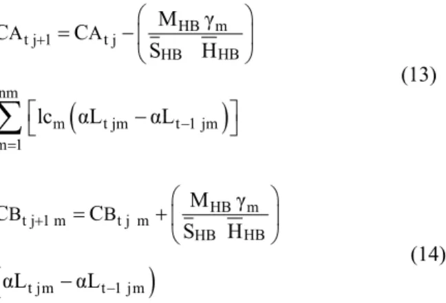
Figure 1: a) Schematic representation of the solution flow model describing the calculation sequence of the chemical species solution content (Ctj and Ctj+1) and the residual chemical species bed content (Jtj)
for a heap with three layers, where the simulation time (t) is set as a multiple of the average residence time of the solution in the bed (W). b) Schematic representation of the solid-liquid reacting system
showing the unreacted core composed by a reactive specie (B) and an inert matrix (S), the reacted shell composed only by an inert matrix, and the liquid reactant (A)
Solid-Liquid Kinetic Model
Considering a spherical low porosity solid-liquid reaction system of radius R, see Fig. 1b, composed by a liquid reactant (A) that surrounds an inert and a reactant solid (B) reacting following the kinetic equation: rA= lcA/B rB= lcA/B kSCACBo, where r is the
reaction rate, k is the rate constant, C is the concentration and lc is the individual reactive consumption factor; when the diffusion process is slow compared with the reaction and the density variation of the solid particle is negligible, the solid reactant recovery (D%) can be approximately described by the following ordinary differential equation, instead of a system of partial differential equations (Froment and Bischoff, 1990):
A Bo B 2 1 3 B Ae 2 3 BS Bo ls ls
3 C lc C dĮ
dt R
1 Į 1
D
R R
1 Į
lc k C k A
§ · ¨ ¸ © ¹ #
§ · ª º
¨ ¸
¨ ¸ «¬ »¼
© ¹ § · ¨ ¸ © ¹ (2)
with the initial condition: t = 0 DB = 0
The three terms in the denominator of this Eq. 2 represent respectively the rate control by diffusion, by chemical reaction, and by mass transfer through the liquid boundary diffusion layer. In many heap leaching operations, the large size of the particles and their relatively low porosity cause a predominance of the diffusive control, thus this equation, for species, layer and multi-size leaching system can be simplified to:
t ji m t ji m
1 3 t ji m
d K
dt
1 Į 1
D
(3)
where,Dtjim is the recovery of the chemical specie m
in the size fraction i of layer j in time t, and Ktjim is
the kinetic parameter, function of time, given as:
t j A
t ji m 2
i T
A
3 C D
K
R lc (4)
where, CAtj is the concentration of the leaching
agent in the solution that enters in layer j at time t, DA is the apparent diffusivity of the leaching agent
in the solid particles, Ri is the average radius of the
solid particles of the size fraction i, and lcT is the
leaching agent consumption factor, which, after Box and Prosser (1986) and Prosser (1989), for multi-species system can be estimated from the individual leaching consumption factors (lcm) as follows:
nm
T m m m
m 1
lc ȡ
¦
lc Ȗ ș (5)where, U is the solid particle density, Jm is the
average initial concentration of the specie m in the solid, and Tm is the maximal recovery by leaching of
the specie m in the solid; alternatively, the individual leaching consumption factors can be estimated from the leaching consumption factor as follows:
nm
T m m
m
m m
m m m 1
lc F F
lc W W ș Ȗ § · ¨ ¸ ¨ ¸
©
¦
¹ (6)where Wm is the atomic or molecular weight of the
leachable specie m and Fm is the dissolution
stoichiometric factor for the specie m.
Equation 3 can be analytically integrated to give the individual specie recoveries (Dtjim) from the size
particles i, localized at layer j, at time t·'W (corresponds to the solution residence time in each heap layer), when the values of the species recovery at the previous time (Dt-1jim), the leaching
concentration from previous layer (CAtj-1) and the
individual concentrations of the species in the bed (Jmj) are known; the resulting equation is given by:
3 2
t ji m t ji m t ji m t ji m tji m t ji m
Į b Į c Į d 0 (7)
where:
t ji m t ji m
b Z 3 227 8;
2 t ji m t ji m
c Z 3 4 27 4 ; (8a,b,c,d)
3 t ji m t ji m
d Z 1 8 27 8 ;
2 3t ji m t ji m t 1 ji m t 1 ji m
Z 2 K ǻIJ3 1Į 2Į
determined, must be used to take into account this effect:
t ji m t ji m m
Į' Į ș (9)
The global recovery in each layer (DLtjm) at
each time increment can be calculated by using the particle size distribution (fi), assumed
homogeneously distributed in each one of the nl layers, considering that there are no variations in the particle chemical content at the time increment that Eq. 7 is solved:
nf
t jm t ji m i i 1
ĮL
¦
Į' f (10)Assuming that each of the nl layers of the heap has the same weight, the global recoveries of each chemical species, at each time increment (D+tm), are
given by:
nl nl
t m t jm jm jm
j 1 j 1
ĮH
¦
ĮL Ȗ¦
Ȗ (11)The residual content of each specie in each layer of the heap (Jrtjm) can be calculated at time t, using
the initial concentration of the specie m, located in layer j (Jojm) and the global recovery in each layer
(DLtjm) as follows:
t jm o jm t jm
Ȗr Ȗ 1ĮL (12)
The leaching agent and the metal species concentration in the solution that leave the layer j are calculated using the mass balance of the species in the layers and the bed hold-up given by Eq.1, as follows:
HB m t j 1 t j
HB HB nm
m t jm t 1 jm
m 1
A A M Ȗ
C C
S H
lc ĮL ĮL
§ ·
¨ ¸
© ¹
ª º
¬ ¼
¦
(13)
HB m t j 1 m t j m
HB HB
t jm t 1 jm
B B M Ȗ
C C
S H
ĮL ĮL
§ ·
¨ ¸
© ¹
(14)
where CAtj and CAtj+1 are the concentrations of the
leaching agent in the solution that enters and leaves
layer j at time t, CBtjm and CBtj+1m are the
concentrations of the metal m in the solution that enters and leaves layer j at time t, DLtjm, and DLt-1jm
is the recovery of the metal m in layer j at the present time and at the previous time, MHB is the
heap weight, HHB is the average heap height, and
HB
S is the average heap top surface.
In partial summary, the proposed mathematical model to the heap and column leaching process uses a diffusive control model to describe the solid-fluid reaction and the plug flow assumption to describe the solution flow in the particles bed. It considers that the leaching solution enters on the top of the heap in the first layer, where it remains for a duration of time equal to the average residence time in the bed divided by the number of layers, which are the same to all other layers. Later, the solution is transferred to the next layer and from this to the next until it reaches the last one. During the amount of time that the liquid solution remains in each layer Eq. 7 is solved for each chemical species contained in each size-fraction, by taking into account the residual specie contents and the composition of the solution. After that, Eqs. 9 to 14 are used to update the residual content of the chemical species in the solid particles and in the solution; the algorithm details, the main elements of the simulation code, and an analyzis of the performance and the results for the cases studies presented by Box and Prosser (1983), for which the present algorithm gives similar results and shorter simulation times, can be found in de Andrade Lima (1992).
SENSITIVITY ANALYSIS OF THE MODEL
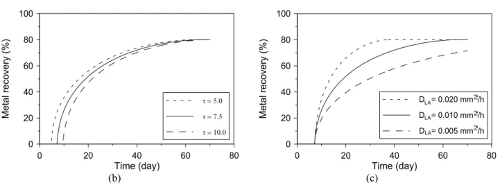
For the sake of conciseness, in this paper only the analysis of the effects of the main variables in the performance of the model are presented; however, for a detailed sensitivity analysis of this model the reader is reported to de Andrade Lima (1992).
Table 1 presents the gold heap leaching simulation variables to seven cases that will be analyzed in this section; these variables are the leaching agent apparent diffusivity (DAL), the solid
particles density (U), the leaching agent consumption factor (lcT), the solid metal content (JM), the
passivation factor for the metal (TM), the solid bed
length (HHB), the solid bed weight (MHB), the solid
irrigated flowrate per surface unit (Q SHB ), the
average particles size (R), and the number of layers (nl). The first column of Table 1 shows the reference case used for comparison with the other cases; in columns 2 and 3 the number of heap subdivisions are changed from 20, in the reference case, to respectively 5 and 50; in columns 4 and 5 the apparent diffusivity of leaching agent is changed
from 0.010 mm2/h, in the reference case, to
respectively 0.005 and 0.020 mm2/h; in columns 6 and 7 the average residence time of the solution in the heap is changed from 7.5 days, in the reference case, to respectively 5 and 10 days.
The calculated results for the time evolution of metal recovery and metal concentration in the solution are summarized in Figs. 2 and 3. One remarks in Fig.2a and 3a that the number of layers does not substantially affect the calculated results for metal recovery neither the metal concentration in
solution after a critical value. In addition, one remarks in Fig. 2b and 3b that the average residence time of the solution in the heap impacts strongly the calculated results for metal recovery and metal concentration in solution and also the metal concentration in the first fractions of the pregnant leach solution recovered. Finally, one notes in Fig. 2c and 3c that the apparent diffusivity of leaching agent strongly impacts the calculated results for metal recovery and the solution metal content. Since the apparent diffusivity of the leaching agent and the average residence time of the solution in the heap affect substantially the simulations results and due the fact that in industrial operations, as these presented in cases studies 1 and 2 in the next section, these parameters are not well known they were chosen in this work as estimated parameters of the model. These parameters may eventually be correlated with process variables using reliable empirical correlations, as attempted by Box and Yusuf (1984), but this beyond the scope of the present work.
Table 1: Input data for the sensitivity analysis simulation runs.
1 2 3 4 5 6 7
DLA [mm2h-1] 0.010 0.010 0.010 0.005 0.020 0.010 0.010
U [g cm-3] 2.7 2.7 2.7 2.7 2.7 2.7 2.7
lcT [g kg-1] 0.40 0.40 0.40 0.40 0.40 0.40 0.40
JM [g t -1
] 3.00 3.00 3.00 3.00 3.00 3.00 3.00
TM [%] 80.0 80.0 80.0 80.0 80.0 80.0 80.0
HB
H [m] 4.7 4.7 4.7 4.7 4.7 4.7 4.7
MHB [t] 15000 15000 15000 15000 15000 15000 15000
HB
S [m2] 2500 2500 2500 2500 2500 2500 2500
W [day] 7.5 7.5 7.5 7.5 7.5 5.0 10.0
CLA [g L -1] 1.2 1.2 1.2 1.2 1.2 1.2 1.2
HB
Q S [L h-1 m-2] 5.0 5.0 5.0 5.0 5.0 5.0 5.0
R [mm] 9.525 9.525 9.525 9.525 9.525 9.525 9.525
nl 20 5 50 20 20 20 20
0 20 40 60 80
Time (day)
0 20 40 60 80 100
M
e
tal r
e
covery
(%)
nl = 5
nl = 20
nl = 50
0 20 40 60 80
Time (day)
0 20 40 60 80 100
Metal reco
very
(%
)
W
W
W
(b)
0 20 40 60 80
Time (day)
0 20 40 60 80 100
Metal reco
very
(%
)
D = 0.020 mm /h
D = 0.010 mm /h
D = 0.005 mm /h LA
LA LA
(c)
Figure 2: Sensitivity analysis results of the model showing the effects of three parameters on the metal recovery time evolution: a) Number of layers (nl). b) Average solution residence time (W).
c) Effective diffusivity of the leaching agent in the particles (DLA).
0 20 40 60 80
Time (day)
0 2 4 6 8
M
e
tal concentration (mg/L)
nl = 5
nl = 20
nl = 50
(a)
0 20 40 60 80
0 2 4 6 8
M
e
tal conc
entration (m
g/L)
Time (day)
W
W
W
A
BC
(b)
0 20 40 60 80
Time (day)
0 2 4 6 8
Metal concen
tra
tion (mg/L)
D = 0.020 mm /h
D = 0.010 mm /h
D = 0.005 mm /h
LA LA LA
(c)
Figure 3: Sensitivity analysis results of the model showing the effect of three parameters on the metal concentration in solution time evolution: a) Number of layers (nl). b) Average solution residence
SIMULATION RESULTS
As mentioned in previous section, the apparent diffusivity of the leaching agent in the solid particles and the solution average residence time in the solid bed are used to calibrate the proposed model. In this non-linear fit, a conventional optimization method without derivatives is used together with the follows last-square objective function (J), that takes into account the adjust of both simulated variables, the recovery, and the concentration of the chemical specie m, and the number of layers used in the numerical simulation:
2 *
Tmax tm t(nl 1)m
2 *
t 1
tm tm
B B
C C
1 nl
H H
J
Į
Į
ª º
« »
« »
« »
« »
¬ ¼
¦
(15)where, CBtm is the simulated concentration of
chemical specie m in the pregnant solution at time t, DHtm is the simulated global recovery of the
chemical specie m at time t, and nl is the number of layers used in the numerical simulation; the superscript (*) stands for experimental values.
In the next sub sections, two case studies are presented; the first one is a gold ore heap leaching and the second one is an oxidized copper ore pilot column leaching; for more details about the chemical and engineering aspects of these processes the reader is referred to Habashi (1997).
Case 1 - Gold Ore Heap Cyanidation
This first case uses experimental data from the
industrial gold heap cyanidation number 42 operated by Rio Salitre Mining (Companhia Bahiana de Pesquisa Mineral); this heap used the oxidized layer of a gold ore with negligible concentrations of “cyanicides” or “preg-robbers” species (de Andrade Lima, 1992). Table 2 summarizes the values for the variables used in the simulation; note that no detailed data were available in this case to particles size distribution, bed length and irrigated area of the heap; consequently, the nominal values were assumed as truth. The calibration parameters of the model, namely the apparent diffusivity of the leaching agent and the average residence time of the solution in the heap, are also shown in Table 2.
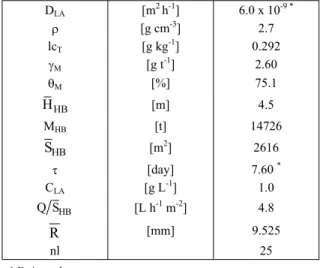
The simulated and experimental results are presented in Fig. 4a and 4b. The simulated results reproduce the general experimental result features, such as the concentration asymptotic exponential decay, after a sharp point, and the correspondent asymptotic exponential increasing recovery; however, there are some biases that may be credited to the kinetic model simplification and specially the assumption of solution flow without dispersion. In Fig. 4a the bias A corresponds to the rapid drainage of the pregnant solution, and the bias B likely is due to the neglecting the size distribution of the ore particles. In Fig. 4b the bias C, the spread in the peak concentration of the gold, is caused by the dispersions of the solution flowing through the heap, and the bias D is due to the recycling of the leach solution, after recovery the gold by activated carbon columns, with a residual gold concentration in the order of 0.5 to 1 parts per million.
Table 2: Input data for Case 1 (Rio Salitre Mining - Heap #42)
DLA [m2h-1] 6.0 x 10⁻⁹ *
U [g cm-3] 2.7
lcT [g kg-1] 0.292
JM [g t-1] 2.60
TM [%] 75.1
HB
H [m] 4.5
MHB [t] 14726
HB
S [m2] 2616
W [day] 7.60*
CLA [g L-1] 1.0
HB
Q S [L h-1 m-2] 4.8
R [mm] 9.525
nl 25
G
o
ld
r
e
c
o
v
e
ry
(
%
)
0 15 30 45 60
Time (day)
0 25 50 75
Observed Calculated
B
A
(a)
Gol
d c
o
n
c
ent
rat
ion
(m
g/
L
)
0 15 30 45 60
Time (day)
0 2 4 6
Observed Calculated
D
C
(b)
Figure 4: Comparison between calculated and experimental data for the industrial gold heap leaching (Case 1): a) Gold recovery time evolution. b) Gold concentration in solution time evolution.
The biases A, B, C and D are explained in the text.
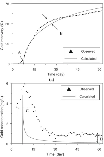
Case 2 – Oxidized Copper Ore Column Acid Leaching
This second case uses experimental data from the oxidized copper ore acid leaching large pilot column number 1 operated by Gaspé Mining Division (Noranda Mines and Exploration Inc); this column used a oxidized copper ore which characterization showed that 96% of the copper is malachite, 3% is chrysocolla and 1% is chalcopyrite, 23.7% of the ore is carbonated material, 65% are silicates, and 11.3% are sulfides (Comeau, 1996). The original experimental results of copper recovery from liquid and solid presented an important bias that restricted a reliable evaluation of the model, so the experimental data set was firstly reconciled using the classical Lagrange multipliers method (Narasimhan and Jordache, 2000). Table 3a summarizes the variables
used in the simulation; note that the maximum copper recovery is the nominal value that is assumed as truth; Table 3b presents the particle size distribution for each size fraction of the ore in the column. The two calibration parameters of the model, namely the apparent diffusivity of the leaching agent and the average residence time of the solution in the column, are also shown in Table 3a.
drainage of the pregnant caused by channeling and axial dispersions of the solution flowing through the column; in Fig. 5b the bias B, the slope in the peak concentration of the copper, is caused by the
dispersions of the solution flowing through the column, and the bias C is due to the recycling of the leach solution, after recovery the copper by solvent extraction, with a residual copper amount.
Table 3a: Input data for Case 2 (Gaspé Mining Division - Large Column #1)
DLA [m2h-1] 1.43 x 10⁻⁷ *
U [g cm-3] 2.7
lcT [g kg-1] 14.60**
JM [%] 1.791**
TM [%] 100
HB
H [m] 3.0
MHB [t] 2.592
HB
S [m2] 0.393
W [day] 5.36*
CLA [g L-1] 10
HB
Q S [L h-1 m-2] 11.216**
nl 10
*Estimated parameter ; ** Reconciled parameter
Table 3b: Size distribution for Case 2 (Gaspé Mining Division - Large Column #1) R [mm] 127.0 101.6 76.20 50.80 25.40 19.05 12.70 6.350 0.296 0.209 0.148 0.146 0.074 0.052
f [%] 6.22 2.22 2.00 6.41 22.55 9.68 14.46 17.77 6.80 1.24 0.93 1.14 1.42 7.18
0 20 40 60
Time (day)
0 25 50 75 100
Observed
Calculated
Copper r
e
covery
(
%
)
A
0 20 40 60 Time (day)
0 4 8 12 16 20
Observed
Calculated
C
op
per c
on
c
ent
rat
ion
(g/
L)
C B
(b)
Figure 5: Comparison between calculated and experimental data for a pilot column oxidized ore acid leaching (Case 2): a) Copper recovery time evolution. b) Copper concentration time.
CONCLUSIONS
Isothermal heap and column leaching processes are mathematically described by using a comprehensive model that takes into account the solution flow in the solid bed, assumed as unidirectional without dispersion, and the solid-fluid reaction, assumed as under diffusive control. The solid bed is than numerically divided into plane layers and the recovery of the chemical species, and the enrichment of the pregnant leach solution are calculated from interactions among these layers.
The sensitivity analysis of the model show that the apparent diffusivity of the leaching agent in the solid particles and the average solution residence time in the solid bed are parameters that strongly impact the simulation results; these parameters are used to calibrate the model. Despite some biases due to the model simplification, the simulations of an industrial gold heap leaching and a pilot column copper acid leaching showed that the model can successful predict the general features of the process time evolution and can be used to general design studies.
ACKNOWLEDGMENTS
The author would like to thank National Council of Scientific Development of Brazil (CNPq) for a scholarship and Rio Salitre Mining (Companhia Bahiana de Pesquisa Mineral) and Mines Gaspé
Division (Noranda Mines and Exploration Inc.) for providing experimental data.
REFERENCES
Box, J.C. and Yusuf, R. (1984). Simulation of heap and dump leaching process, Proceedings of the Symposium on Extractive Metallurgy, Melbourne, Australia, p.117-124
Box, J.C., and Prosser, A.P. (1986). A general model for the reaction of several minerals and several reagents in heap and dump leaching. Hydrometallurgy, 16, 77-92.
Cathles, L.M. and Apps, J.A. (1975). A model of the dump leaching process that incorporates oxygen balance, heat balance, and air convection, Metallurgical Transactional B, 6B, 617-624. Cathles, L.M. and Schlitt, W.J. (1980). A model of
the dump leaching process that incorporates oxygen balance, heat balance, and two dimensions air convection, Proceedings of the Las Vegas Symposium on Leaching and Recovery Copper from As-Mined Minerals, Edited by Schlitt, W.J., p.9-27.
Davis, G.B. and Ritchie, A.I.M., (1986). A model of oxidation in pyritic mine wastes: part 1 - equations and approximate solution, Applied Mathematical Modelling, 10, 314-322.
Davis, G.B., Doherty, G.B. and Ritchie, A.I.M. (1986). A model of oxidation in pyritic mine wastes: part 2 - comparison of numerical and approximate solution, Applied Mathematical Modelling, 10, 323-329.
de Andrade Lima, L.R.P. (1992). Simulation of gold ores heap leaching, M.Sc. Thesis, COPPE/UFRJ, Rio de Janeiro, Brazil, 235pp. (in Portuguese) Dixon, D.G. and Hendrix, J.L. (1993). A
mathematical model for heap leaching of one or more solid reactants from porous ore pellets, Metallurgical Transactions, 24B, 1087-1102. Froment, G.F. and Bischoff, K.B. (1990). Chemical
reactor analysis and design, 2nd edition, John While and Sons, New York, 664pp.
Habashi, F. (1997). Handbook of Extractive Metallurgy, Wiley-VCH, Germany, 2426pp. Narasimhan, S., and Jordache, C. (2000). Data
reconciliation & gross error detection: an intelligent use of process data, Gulf Publishing Company, Houston, 406pp.
Pantelis, G. and Ritchie, A.I.M. (1991). Macroscopic transport mechanisms as a rate-limiting factor in dump leaching of pyritic ores, Applied Mathematical Modelling, 15, 136-143.
Pantelis, G. and Ritchie, A.I.M. (1992). Rate-limiting factors in dump leaching of pyritic ores, Applied Mathematical Modelling, 16, 553-560. Pantelis, G., Ritchie, A.I.M. and Stepanyants, Y.A
(2002). A conceptual model for the description of
oxidation and transport processes in sulphidic wast rock dumps, Applied Mathematical Modelling, 26, 751-770.
Petersen, J and Petrie, J.G. (2000). Modelling and assessment of the long-term leachate generation potential in deposits of ferro-chromium slags, The Journal of the South African Institute of Mining and Metallurgy, 100, 369-378.
Petersen, J and Dixon, D.G. (2002). Systematic modelling of heap leaching processes for optimisation and design, Proceedings of the EPD Congress 2002 and Fundamentals of Advanced Materials for Energy Conversion, Edited by Taylor, P.R., Chandra, D., and Bautista, R.G., TMS, p.757-771.
Prosser, A.P. (1989). Simulation of gold heap leaching as an aid to ore-process development, Proceedings of the Precious Metals'89, p.121-135.
Roman, R.J., Benner, B.R., and Becker, G.W. (1974). Diffusion model for heap leaching and its
application to scale-up, Transactions of the Society of Mining Engineers of AIME, 256, 247-256. Roman, R.J., Figueroa J. H. P., Ruiz, J.E.H.,
Helleon, J. G., Perez, E.S. (1999). Interpretation of the recovery/time curve and scale-up from column leach tests on a mixed oxide/sulfide copper ore, Proceedings of the Copper 99 International Conference, Edited by Young, S.K., Dreisinger, D.B., Hackl, R.P. & Dixon, D.G., Phoenix, Arizona, USA, Vol. 4, p. 453-466. Sánchez-Chacón, A.E. and Lapidus, G.T. (1997).