Braz. J. Chem. Eng. vol.21 número3

ISSN 0104-6632 Printed in Brazil

Vol. 21, No. 03, pp. 367 - 392, July - September 2004

Brazilian Journal

of Chemical

Engineering

MEASUREMENT PROCESSING FOR STATE

ESTIMATION AND FAULT IDENTIFICATION IN

BATCH FERMENTATIONS

R. Dondo

Instituto de Desarrollo Tecnológico para la Industria Química, INTEC (CONICET-UNL), Güemes 3450 (3000) Santa Fe, República Argentina.

E-mail, rdondo@ceride.gov.ar

(Received: January 6, 2003 ; Accepted: March 9, 2004)

Abstract - This work describes an application of maximum likelihood identification and statistical detection

techniques for determining the presence and nature of abnormal behaviors in batch fermentations. By appropriately organizing these established techniques, a novel algorithm that is able to detect and isolate faults in nonlinear and uncertain processes was developed. The technique processes residuals from a nonlinear filter based on the assumed model of fermentation. This information is combined with mass balances to conduct statistical tests that are used as the core of the detection procedure. The approach uses a sliding window to capture the present statistical properties of filtering and mass-balance residuals. In order to avoid divergence of the nonlinear monitor filter, the maximum likelihood states and parameters are periodically estimated. The maximum likelihood parameters are used to update the kinetic parameter values of the monitor filter. If the occurrence of a fault is detected, alternative faulty model structures are evaluated statistically through the use

of log-likelihood function values and χ2 _{detection tests. Simulation obtained for xanthan gum batch}

fermentations are encouraging.

Keywords: fermentation process, stochastic model, maximum likelihood state.

INTRODUCTION

The importance of on-line monitoring of biotechnological processes has increased during the last twenty years. Advantages include gaining knowledge about the state of the process and the possibility of detecting and isolating abnormal process developments at early stages. This reduces process costs, contributes to process safety and helps in trouble-shooting and process accommodation. The main problem in fermentation monitoring and control is the fact that process variables usually cannot be measured on-line (e.g., biomass, substrate and product concentrations). Monitoring and controlling these processes can therefore be difficult because only indirect measurements are available on-line, while calculated values may be rather uncertain.

This can be due to uncertainty with respect to the equations used, measurement errors or both. For automatic control this may have serious consequences, especially as the actual variables of interest often cannot be directly controlled and related variables are controlled instead.

due to minor disturbances in the measurement equipment. The magnitude of these errors, commonly referred as measurement noise, defines the accuracy of the measurement. They are usually regarded as zero-mean with Gaussian distribution. This kind of noise can be eliminated by the use of state estimators such as Kalman filters. On the other hand, multi rate estimators [Halme, 1987] are observers that are well suited for state estimation in fermentations. In these estimators, the measurement vector is expanded to include infrequent off-line measured variables when these measurements are available. This expansion is only made functional at the time of measurement. To overcome problems with the time delay caused by laboratory analysis the technique uses stored data. The estimates are then recalculated from the time of measurement to the present as soon as the measurement value becomes available. In many cases, there is a certain amount of “overlap” between off-line and on-line measurements. This overlap together with conservation equations provides constraints to improve the accuracy of the measurements and to detect signific ant errors in the measurements or in the model used by the fermentation observer. Faulty sensors and omitted components can be detected in this way. This results in enhanced reliability and accuracy of on-line state and parameter estimates.

Much research on state estimation in bioprocesses can be found in the literature. Some of the most relevant are by Stephanopoulos and San [1984a and b], Bastin and Dochain [1986, 1990] and Gudi et al. [1994]. Two different detection methods can be used for fault detection in batch fermentations. The first is herein referred to as the “residual-based detection method”. It focuses on the analysis of estimation residuals of a Kalman-filter-type observer. The second is herein referred to as the “balance-based detection method” and it uses conservation principles for testing the consistency of the variables measured. Isermann [1984] and Frank [1990] offer survey of the residual-based detection method. Alcorta García and Frank [1997] reviewed observer based approaches to several classes of deterministic nonlinear systems. Significant works related to the balances-based detection method were published by Wang and Stephanopoulos [1983] and Van der Heijden [1994a and b]. Dondo [2003] proposed the simultaneous use of both methods. The idea behind the use of both methods is that the limitations of one be compensated by the use of the other. In the present work an evolution of the idea developed in Dondo [2003], which is designed for obtaining robust and accurate state estimation and fault

diagnostics under parametric uncertainty, is presented.

This work is organized as follows: section 2 discusses the specifics of estimation and detection in batch fermentations. In section 3, a methodology of state estimation and fault detection for batch fermentations is presented. Numerical results are shown in section 4 and the conclusions are outlined in section 5.

PROBLEM DISCUSSION

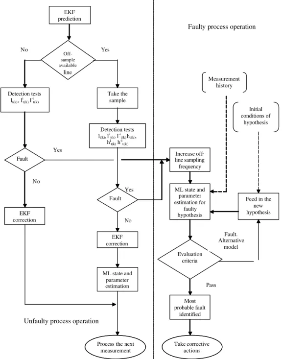
Instrumentation failures and abrupt kinetic changes can be understood as a deviation of a process variable that is not permitted and that leads to an inability to maintain control of the running fermentation. In the present work, these deviations are generically referred to as faults. Fig. 1 shows a block diagram for fault detection and isolation in fermentations. Checking whether measured and/or unmeasured estimated variables are within a given tolerance of their normal values means detection. If the check is not passed, this leads to a fault message. Tasks related to detection and isolation can be divided into the following stages:

§ Residual generation: computation of functions

that are sensitive to the occurrence of a fault.

§ Fault decision: checking residuals if there is a fault.

§ Fault isolation: identification of fault occurrence time, type, size and source.

Computational requirements are a practical problem regarding fault detection because algorithms for detection and diagnosis are often computation intensive. Nevertheless, this is not a problem for the reason that batch-fermentations are generally carried out over many hours or even days. Furthermore, a detection algorithm must have two important capabilities:

§ The ability to quickly detect the occurrence of an abnormal event within a short period following its occurrence.

§ The ability to correctly identify the event, its occurrence time and its magnitude.

§ One of the fundamental aims of supervision of a biotechnological process is to promptly detect and identify abnormal behaviors (faults) in order to take corrective action for maintaining the fermentation running. This capability is crucial for enhancing the reliability of the operating equipment and to ensuring a profitable operation. Examples of sources of faults in batch fermentations are

§ The system description is incorrect because a component has a composition different from that specified or a component is not included in the description of the fermentation.

§ Abrupt kinetic changes are produced during the course of the fermentation.

§ The assumed measurement variances are

incorrect resulting in a poorly tuned estimation algorithm.

§ Since detection methods must be sensitive to the occurrence of faults but robust to noises, modeling

errors and signal variations, the following trade-off exist [Isermann, 1984]:

§ Size of faults vs. detection time.

§ Parameter estimation rate vs. false alarm rate. § Detection time vs. false alarm rate.

Methods that are designed for detection of abrupt changes are usually not suitable for state and parameter estimation and vice versa. These considerations call for developing an innovative approach and have motivated the methodology presented below.

Figure 1: Conceptual structure of the methodology for fault detection and isolation in fermenters

THE ESTIMATION AND DETECTION METHODOLOGY

An aerobic fermentation with production of a single metabolite can be seen as three parallel “chemical reactions” denoted partial metabolisms [Minkevich, 1983]. These reactions are biomass production, metabolite production and main substrate oxidation. Thus, the aerobic growth of biomass (X) consuming a carbon and energysource (S) and an independent nitrogen source that can also contain carbon (SN) while generating a metabolite P, CO2,

and H2O can be written as

Biomass production:

a 2 b2 c2 d 2 a 4 b 4 c 4 d 4

X / S X / N

b1 c1 d1 2 2

X / H 2 O X / C O 2

1 1

C H O N C H O N

Y Y

1 1

C H O N H O C O

Y Y

+ →

+ +

(1.a)

Metabolite production:

a 2 b 2 c2 d 2 2

P / S P / O 2

a 3 b 3 c3 2 2

P / H 2 O P / C O 2

1 1

C H O N O

Y Y

1 1

C H O H O C O

Y Y

+ →

+ +

(1.b)

Main substrate oxidation:

a 2 b 2 c 2 d 2 2 S / O 2

2 2

S / C O 2 S / H 2 O

1

C H O N O

Y

1 1

CO H O

Y Y

+ →

+

Compositions of components X, S, P and SN are

expressed by their atomic formulae CHb1Oc1Nd1,

Ca2Hb2Oc2Nd2,, Ca3Hb3Oc3 and Ca4Hb4Oc4Nd4,

respectively (the metabolite is assumed to be a nitrogen-free component). The kinetics of each reaction are characterized by the evolution of each one of the relevant reaction components: X, P and SR

N

X / S X / N X / C O 2 X/H2O ₂

P / S P / O 2 P/CO2 P / H 2 O

P / O 2 S/CO2 S/H2O ₂

2

S S 1 1 _{0 1 0} 1 1

Y Y Y Y _{O 0}

1 ₀ 1 _{0 1} 1 1 _{X 0}

Y Y Y Y

0 P

1 1 1

1 0 _Y 0 0 _{Y Y}

CO H O

∆

 

_∆ 

 _{  }

 _{ ∆   }

 _{    }

= ∆

 _{    }

 _{  ∆    }

 _{  }

  ∆

   

_∆ 

 

 

(2.a)

or

I / J

Y

C ∆ =I 0 (2.b)

where CY I/J is a matrix of stoichiometric yields YI/J

and ∆I is a vector of net production of the system components. Since element balances are constraints that must always be satisfied, they are constraints to be met by the fermentation “reactions”. These balances mean four constraints (one for each element considered: C, H, O and N) to be met by the relation between seven components (X, S, P, SN, O2, CO2 and

H2O). Thus, an aerobic fermentation with formation

of a single metabolic product has ( 7-4 ) = 3 degrees of freedom and unknown component evolutions may be obtained from the knowledge of the stoichiometric yields YI/J and three component

evolutions. Thus, if there are more than three measurements of component evolutions, an overlap of measurements is produced. This overlap and conservation equations (2) provide constraints to improve the accuracy of measurements and to detect significant errors in measurements or in the model used by a fermentation observer. In this way, constraints (2) can be lumped into a conventional detection methodology for building an efficient estimation and detection procedure. To do this, let us assume that the dynamic model of a batch fermentation is represented by the usual nonlinear state-space formulation:

x f(x,u,p)•= (3.a)

y c(x)= (3.b)

In this formulation, kinetic parameters p appear in the dynamic function f(•), while if some of the fermentation components are measured, balances constraints are in the state-measurement relations c(•) [Dondo and Marqués, 2002]. In order to explain this, let us assume that the fermentation states are the biomass concentration [X], the metabolic product concentration [P] and the amount of main substrate oxidized (∆SR_{). The amount of oxygen consumed}

(∆O2) and the amount of carbon dioxide produced

(∆CO2) are on-line measurements, and the biomass

concentration [X], the metabolic product concentration [P] and the main substrate concentration [S] are off-line measurements. This is probably the most common measurement arrangement in batch fermenters. From expression (2.a) it is clear that the relation between these main components is linear. Thus, the relation between states and measurements is also linear [Dondo and Marqués, 2002], and it can be expressed as the product of a matrix of stoichiometric coefficients C by the vector of states xt(k):

t(k) t(k)

y =Cx (4.a)

[ ]

[ ]

[ ]

t ( k )

P / O 2 S / O 2 0

2

t(k) 2 on line

X / C O 2 P/CO2 S/CO2

0 _{on line}

0

X / S off line t(k)

off line _t(k)

1 1

0

OURdt Y Y

O

1 1 1

CO

CPRdt _{Y Y Y}

S

1

S S

X _Y

X P

P

−

−

−

−

  

  

 ∆   _{  }

_{∆ } 

  

 

  _{ }

 

 _{∆ }  _=  _{ =}

 _{ }  _{  −  }

 _∆ _  _{   }

 

 _∆ _     

  _{   }

 

 

∫

∫

R t(k) P / S

X X P 1

1 _S

Y

1 0 0

0 1 0

 

 

 

 _{  }

−

 _{  }

 _{  }

 _{  }

 _{  }

 

 

 

 

 

Since most kinetic models of batch fermentations are nonlinear and have parametric uncertainty, adaptive nonlinear observers are used for monitoring this kind of processes [Gudi et al., 1994; Dondo, 2003]. Although the use of off-line information within the adaptive estimation procedure makes the estimates more robust, the uncertainty of estimated variables (given by the state covariance matrix) is relatively high [Dondo, 2003]. This uncertainty is also manifested as high values of the measurement covariance matrix and reduces the sensitivity of any detection test [Wilsky, 1986]. Hence, hypothesis distinguishibility is rather difficult. Consequently, to promptly detect a fault, a sensitive logic that takes into account the past history of the system as well as parametric uncertainty must be designed. The approach to the estimation and detection problem presented here relies on an intensive use of statistical

criterions as indicators of a faulty process. These criterions are based on “signatures” of the fermentation which are monitored and compared with a priori estimations based on the unfaulty model of the system. Statistical indicators are also used to determine the occurrence time of faults and their identity. The operative logic of the estimation-detection procedure is detailed in the following subsections.

Normal Process Operation

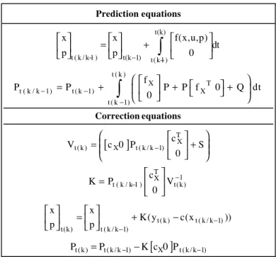
Let us assume that a multi rate extended Kalman filter (EKF) is used as fermentation states and parameters estimator (Table 1). The innovation sequence of the filter is defined by

t(k) yt(k) c(xt ( k / k 1)− )

γ = − (5)

Table 1: The EKF as state and parameter estimator

Prediction equations

t(k) t ( k / k 1 ) t(k 1) _t(k1)

x x f(x,u,p)

dt

p ₋ p ₋ 0

−

  ₌  ₊  

     

   

∫

t ( k )

X T

t ( k / k 1) t ( k 1) X

t ( k 1)

f

P P P P f 0 Q dt

0

− −

−

  _{ } 

= + _{ } + _{ } + _

 

 

∫

Correction equations

[

]

t(k) X t ( k / k 1)

c

V c 0 P S

0

−

   

=_  + _  

 

T 1 X t ( k / k 1 ) c t(k)

K P V

0

− −  

=  

 

t(k) t ( k / k 1) t(k) t ( k / k 1)

x x

K(y c(x ))

p p ₋ −

  ₌  _{+ −}

   

   

[ ]

t(k) t ( k / k 1) X t ( k / k 1)

P =P ₋ −K c 0 P ₋

In a multirate EKF, the dimensions of vectors yt(k) and c(xt(k/k-1)) change in accordance with the available measurements

where yt(k) is the measurement vector value at time

t(k) and c(xt(k/k-1)) is the prediction of the

measurement vector value based on prediction of the state vector value xt(k/k-1). If there are no convergence

problems and under the no-fault hypothesis (the model corresponds to the reality and the measurements are unbiased and corrupted by independent sequences of “white noises”), sequence γt(k), should be a zero-mean Vt(k) covariance

sequence, where Vt(k) is defined by

T X t(k) X t ( k / k 1) c

V c 0 P S

0

−  

 

=_{ }  +

 

 

(6)

In eq. (6), cX is the Jacobian matrix of c(xt(k/k-1)),

Pt(k/k-1) is the predicted state-covariance matrix at

time t(k) and S is the matrix of noise variances of the measurement vector. Faults and abrupt dynamic changes are usually manifested as unexpected values

indicates a possible fault. For testing the zero-mean hypothesis, the following statistical indicators are proposed:

t(j) t(j)

T 1

k

t(j) t(k)

t(j) j k w 1

V 1

l

w m

−

= − +

γ γ 

 

=

 

 

∑

2 i k

t(j) i

t(k) _i 2

j k w 1 _t(j) 1

l

w _{= − + v}

_γ 

 

=

 

 

∑

t(j) t(j)

T 1

i i i

k _t(j)

i t(k)

t(j) j k w 1

V 1

l

w m 1

−

− − −

−

= − +

_{γ γ} 

 

= _{ }

−

 

 

∑

In eq. (7.a), lt(k) represents the sum of normalized

squared innovations on time horizon w and mt(j) is

the dimension of the measurement vector at time t(j). In eq. (7.b), li

t(k) is the sum on time horizon w of the

squared innovations of measurement i normalized by their variances vi2. Finally, l-it(k) represents the sum of

normalized squared innovations of all but i measurements on time horizon w. The measurement covariance Vt(j) is computed by the EKF. Matrix V -i

t(j) and the variance νit(j)2 are extracted from Vt(j). For

a selected window size, w, the effect on residuals at times t(j) ≤ t(w) is neglected. Under the no-fault-hypothesis, variables lt(k), lit(k) and l-it(k) should be χ2

distributed variables with Σw

j=1 mt(j), w and Σj=1w

(mt(j)-1) degrees of freedom, respectively. Therefore,

by defining thresholds ϕ, ϕi _{and ϕ}-i _{with confidence}

levels selected a-priori, it is possible to carry out the

following tests:

t(k)

t(k)

l Normal operation

l Abnormal operation

≤ ϕ ⇒

> ϕ ⇒ (8.a)

i i

t(k)

i i

t(k)

l Normal operation

l Abnormal operation

≤ ϕ ⇒

> ϕ ⇒ (8.b)

i i

t(k)

i i

t(k)

l Normal operation

l Abnormal operation

− −

− −

≤ ϕ ⇒

> ϕ ⇒

Statistical indicators, lt(k), lit(k) and l-it(k), computed

on the w-lag sliding window, provide simple and efficient detection tools. However, since the sliding window involves residuals from nonlinear filters and a limited sample size, actual indicator values will not be exactly χ2_{-distributed. Detection thresholds cited}

above, which are based on asymptotic properties, should therefore be approximate. Thus, persistence tests (the indicators must exceed their thresholds over a given time period) should be used to cut down false alarms due to spurious and unmodeled events.

In order to avoid convergence problems due to the effect of nonlinearities and to keep variables lt(k),

li

t(k) and l-it(k) sensitive to occurrence of a fault, the

value of Pt(k/k-1) must be keep as small as possible

[Dondo, 2003]. For this purpose, each time that there is an off-line measurement available, a maximum likelihood optimization is used in a time window Ω = t(0),...,t(k):

(

)

(

)

0 t(j) t(k)

T ₁

t(j) t ( j / j 1 ) t(j) t(j) t ( j / j 1 ) t(j) t(j) t

1

max L(p) y c(x ) V y c(x ) ln V

2

=

−

− −

=

 

 

= − − − +

 



∑

(9)

subject to

[ ]

[ ]

x ₋ x ₋ f(x,u,p)dt

−

= +

∫

(

)

t ( j )

T t ( j / j 1 ) t ( j 1 ) X X

t ( j 1 )

P ₋ P ₋ f P P f Q dt

−

= +

∫

(

)

t(j) X t ( j / j 1 ) X

V = c P ₋ c +S (10.c)

T 1

t ( j / j 1 ) X t(j)

K =P ₋ c V− (10.d)

[ ]

[ ]

t(j) t ( j / j 1 ) X t ( j / j 1 )

P =P ₋ −Kc P ₋ (10.f)

This maximization fulfills two tasks: (i) it keeps estimated parameters as near as possible to the true parameter values to avoid divergence of the EKF monitor and (ii) it keeps the covariance matrix Vt(k)

l-i

t(k) sensitive to minor variations in the innovation

sequence. This permits use of small sliding-window lags, w, and then variables lt(k), lit(k) and l-it(k) will be

able to quickly react to an unexpected event. The use of small sliding windows is critically necessary because of the use of adaptive observers. This is because effects of unexpected measurement values on innovations are manifested as correction of the estimated parameter values and will promptly disappear. Maximization (9) had been a very difficult task, particularly in the case of nonlinear systems [Young, 1981]. Main difficulties reported in the literature are the need for considerable computational power and the computation of analytical Jacobian and Hessian for the maximization algorithm. Nevertheless, these difficulties have been practically overcome because of the tremendous advances in computational power and the development of efficient minimization methods that do not use Jacobian and Hessian matrixes (Downhill simplex method due to Nelder and Mead and Powell’s method [Press et al., 1992]). Since the maximum likelihood estimation gives the min imum-variance estimates [Mendel, 1995] it is utilized for on-line state and parameter estimation in a specified time-window Ω = (t(0) … t(k)) in order to reinitialize the

monitor Kalman filter with minimum variance states and maximum likelihood parameters. Time-window lag, Ω, must be large enough to allow a significant collection of information, but small enough to avoid lumping parameter variations.

On the other hand, if there are redundant state-measurement relations when an off-line measurement is availa ble, the following nonlinear least-squares estimation of states and measurement can be obtained:

1

T T

t(k) _{t(k) X X X t(k) t(k)}

x x c c c y c(x )

∧ −

   

= +_{  } − _ (11)

1 T

t(k) X X X

t(k) T

X t(k) t(k)

y c(x ) c c c

c y c(x )

∧ −

 

= + _{ }

 − 

 

(12)

If the difference between xt(k)

∧

and xt(k) is not

acceptable, it is possible to re-estimate the state and measurement vectors by recalculating eqs. (11) and (12), replacing xt(k) by xt(k)

∧

and c(xt(k)) by yt(k)

∧

, respectively. The procedure can be repeated until no significant modifications of estimates are obtained [Mendel, 1995]. Thus, the following residuals vector

and covariance matrix can be defined as follows [Dondo, 2003]:

t(k) yt ( k ) yt(k)

∧

ε = − (13)

1

T 1 T

X X X X

P_ε = −S Sc _c S c− _− c S (14)

Now the following statistical indicators can be computed:

1 T

t(k)

t(k) t(k)

h = ε P_ε− ε (15.a)

2 i t(k) i

t(k) i

t(k) h =_ε _

σ

 

(15.b)

t(k) 1 T

i i i i

t(k) t(k)

h− = ε− P_ε−− ε− (15.c)

where variance σi2 is extracted from variance matrix

Pε. Variable ht(k)-i is computed using all but the i

measurement and P-i

ε is calculated by eq. (14),

eliminating columns and rows related to measurement i from matrixes S and cX. If the

measurement arrangement is given by eq. (4.b), the Jacobian cX is to be replaced by C, and, for tests ht(k),

hi

t(k), and h-it(k), the nonlinear least-squares eqs. (11)

and (12) are simplified to the linear case:

1

T T

t(k) _t(k)

x C C C y

∧ −

 

=   (16)

1

T T

t(k) t(k)

y C C C C y

∧ −

 

=   (17)

If elements of εt(k) are assumed to be zero-mean

and Gaussian-distributed, under the no-fault hypothesis, ht(k), hit(k) and h-it(k) are approximately χ2

-distributed variables with (n-m), 1 and (n-m-1) degrees of freedom, respectively. Thus, the following tests can be conducted:

t(k)

t(k)

h Normal operation

h Abnormal operation

≤ θ ⇒

> θ ⇒ (18.a)

i i

t(k)

i i

t(k)

h Normal operation

h Abnormal operation

≤ θ ⇒

i i t(k)

i i

t(k)

h Normal operation

h Abnormal operation

− −

− −

≤ θ ⇒

> θ ⇒ (18.c)

In expression (4.b) there are n = 3 states and m = 5 measurements and therefore the degree of redundancy is 2. Furthermore, as there are two on-line measurements (∆O2 and ∆CO2), it follows that

lt(k)O2 = lt(k)-CO2 and viceversa.

Variables defined by eqs. (15), when available, and by eqs. (7) form a set of statistical indicators that provide strong indications of the occurrence of a fault. For example, if on-line measurement i is suddenly biased, lt(k) should indicate the occurrence

of an unexpected event, li

t(k) should show a sharp

increase in its value and l-i

t(k) should be

quasi-invariant to this bias. When an off-line measurement is available, indicators ht(k), hit(k) and h-it(k) should also

have a similar behavior.

Tests (8) and (18) give an intuitive justification not only for use in fault detection, but also for formulating a detection/diagnosis scheme. This approach consists of including in the extended Kalman filter various possible faulty models, estimating their parameters by a maximum-likelihood approach while testing indicators ht(k), hit(k)

and h-i

t(k) for these models and then choosing the

model with the maximum log-likelihood function.

This diagnosis scheme will be detailed in the next subsection.

Faulty Process Operation

If a fault is detected, its cause should be identified. Once the information needed to detect and diagnose faults (residuals and measurement history) has been accumulated, it is necessary to interpret the information in various ways: whether or not there is a failure, the probability of occurrence of a failure and the failure most likely to have occurred. Each hypothesis (i.e., sensor drift, formation of a by-product, etc) will demonstrate a specific time-dependent pattern in measurement evolution and tests lt(k), lit(k), l-it(k), ht(k), hit(k) and h-it(k). The idea

behind this is that the signature of the measurement evolution contains information on the kind and magnitude of the fault. Thus, every suspected fault characterized by a given type (I), identity (J), magnitude (υ) and occurrence time (τ) is simulated, and data from these simulations are used to estimate the faulty model states and parameters and to define hypothesis log-likelihood functions LI,J(υ, τ). The

technique can be viewed as an extension of the generalized likelihood ratio method (GLR) [Wilsky, 1986] to the nonlinear case. The general form of the resulting log-likelihood maximization problem can be written as

(

)

(

)

0

t(j) t(k)

T ₁

I J IJ t(j) t ( j / j 1 ) t(j) t(j) t ( j / j 1 ) t(j)

t(j) t

1

max max max L ( , )

y

c(x, , )

V

y

c(x, , )

ln V

2

=

−

− −

=









υ τ = −

−

υ τ

−

υ τ

+







∑



subject to

[ ]

[ ]

x ₋ x ₋ f (x,u,p, , )dt

−

= +

∫

t ( j ) X

t ( j / j 1 ) t ( j 1 ) _T t ( j 1 ) X

f ( , )P

P P dt

P f ( , ) Q

− −

−

 υ τ + 

 

= + _{ }

+ υ τ +

 

∫

(

)

t(j) X t ( j / j 1 ) X

V( , )υ τ = c( , ) Pυ τ ₋ c( , )υ τ +S (20.c)

T 1

t ( j / j 1 ) X t(j)

K =P ₋ c ( , ) V( , )υ τ υ τ − (20.d)

[ ]

[ ]

t(j) t ( j / j 1 ) X t ( j / j 1 )

P =P ₋ −Kc ( , )Pυ τ ₋ (20.f)

where p denotes the previously estimated parameters of the unfaulty process model and (yt(j) – cIJ(x t(j/j-1),υ,τ)) denotes residuals from the (I, J) faulty-model

filter. Log-likelihood function values LI,J(υ,τ) are

computed for each alternative fault location and structure and are ranked from largest to smallest to assess the appropriateness of a particular hypothesis about the unknown event. In addition, the evolution of indicators ht(k), hit(k) and h-it(k) provides further

a) Detection and Isolation of Significant Measurement Errors (I = 1)

A measurement bias can frequently be found. Then the mean of its measurement noise is different from zero. Sensor drift or inaccurate calibration may cause the bias. This type of error can be disastrous when the measured variable is used to determine another process variable for control purposes and it must be promptly detected. But if on-line measured variable i has a significant error, the i element of the innovation sequence is biased, and therefore the value of lt(k) should increase, a sudden and large

change in the value of li

t(k) is expected and l-it(k)

should remain below its threshold. Furthermore, when an off-line sample is analyzed, ht(k), hit(k), and h -i

t(k) should show a similar pattern. Thus, the error can

be detected by analyzing the behavior of these statistical indicators. Failure parameters are estimated by maximizing the log-likelihood function (19). In the same way, if off-line measured variable i has a significant error, since indicators lt(k), lit(k) and l -i

t(k) cannot be calculated, the value of ht(k) should

increase, a sudden and large change in the value of hi

t(k) is expected and h-it(k) should remain below its

threshold.

If the state-measurement relations of the fermentation observer are given by eq. (4.b), variables lt(k), lO2t(k) and lCO2t(k) allow detection of

significant errors in on-line measurements ∆O2 and

∆CO2. Analogously, variables ht(k), hit(k), and h-it(k)

allow detection of significant errors in off-line measurements ∆S, ∆X and ∆P. In principle two simultaneous but related measurement errors can be detected. For example, if there is a fault in the gas-flow measurement device, ∆O2 and ∆CO2 will have a

correlated bias. Thus lt(k), lO2t(k) and lCO2t(k) indicators

will not trigger the alarm but indicators ht(k), hit(k) and

h-i

t(k) will do it. Since residual vectors are usually

rather inaccurate, a search of two simultaneous error sources will not give trustworthy results. Nevertheless, simulation of a hypothesis with a simultaneous and correlated drift in ∆O2 and ∆CO2

should give the maximum log-likelihood-function value.

b) Detection and Isolation of Incorrect System Descriptions (I = 2)

If the evolution of some system components is measured and introduced into eq. (2.b), due to measurement noises this equality will never be exactly satisfied. It can be better written as

I / J

Y

C ∆ = νI (21)

where ν is a residuals vector. Its expected value under the non-fault hypothesis is 0. But in addition to measurement noises, error in the specified constraint (2) may occasionally be encountered. This may be due to time-varying or ill-defined component composition (i.e., biomass), a component omitted from the balance equation or an alternative metabolic pathway (e.g., partial substrate oxidation). This kind of error will result in incorrect balance constraints and must be distinguished from measurement errors. As adaptive observers are used for monitoring batch fermentations, tests lt(k), lit(k) and l-it(k) are not sensitive

to this type of error. This is because the effect of these errors is manifested as a correction of some parameter values, resulting in residuals close to the zero-mean known-covariance hypothesis. Nevertheless, since the specified matrix CY I/J is incorrect,

indicators ht(k), hit(k) and h-it(k) will trigger alarms. To

summarize, alarms triggered by variables ht(k), hit(k)

and h-i

t(k), while variables lt(k), lit(k) and l-it(k) indicate

normal process operation, can be interpreted as an incorrect system description. Other evidence that permit to detect a composition error are (i) no measurement error can cause a residual vector of the given form and (ii) measurement errors that may cause a residual vector of the given form are checked by tests lt(k), lit(k) and l-it(k) and found to be correct.

Incorrect Component Composition

Composition of X and P (if P is a complex product) may not be exactly known or may be time-varying, resulting in incorrect or time-varying element constraints, e.g., the biomass N content can vary with time. Therefore, the detection and diagnosis of other errors will be rather difficult. Nevertheless, there may be heuristic information that can be used within expressions (2) and (17) for reducing uncertainty about the biomass composition. For example, it is known that the biomass C content is fC ≈ 0.48 with a relative variance of 5% and that

the degree of reduction in the biomass “mol” * _{is γ} X≈

4.25 with a relative variance of 4% [Erikson et al., 1978]. These data together with the elemental composition of S, SN and element balances can be

used to derive linear relationships between Y*X/N,

Y*X/S and Y*X/CO2. With this information and

measurements yt(k), the isolation problem can be

*

P/O2 S / O 2 X/O2

* _{P/CO2 S/CO2}

X/CO2 *

* _{P / S}

X / S

1 1 1

Y Y

Y

1 1 1

Y Y

Y

C _{1 1}

1 Y

Y

1 0 0

0 1 0

 

 

 

 

 

=  

 

 

 

 

 

(22)

Missing Components

An analogous procedure is useful to identify the formation of a suspect by-product. Thus, its isolation can be written as the maximization problem given by eqs. (19) and (20), but now C* includes a column of stoichiometric yields of the suspected by-product q in the measured components:

q/O2 X / O 2 P/O2 S/O2

q/CO2 X/CO2 P/CO2 S/CO2

*

X / S P / S q / S

1

1 1 1 _Y

Y Y Y

1

1 1 1

Y

Y Y Y

C _{1 1 1}

1

Y Y Y

1 0 0 ₀

0 1 0 ₀

 

 

 

 

 

=  

 

 

 

 

 

(23)

The mol of biomass is defined by the formula CHb1Oc1Nd1. The degree of reduction of a mol of biomass

is defined as 4+b1-2c1-3d1 [Erikson et al., 1978].

No distinction can be made between an omitted component and a component composition error. However, many components are precisely defined (O2, CO2 and many times S), a limited number of

components (X and sometimes P) lack a defined elemental composition and a limited number of substances are suspected to be omitted by-products. Thus, if probable composition errors for X and P do not cause residuals of the given form, it can be inferred that a component is omitted from constraints (2). It must be noted that, since the matrix C* defined by eq. (23) has one more column than the matrix C* defined by eq. (22), the degree of freedom is reduced to 1 and therefore the threshold θ has to be corrected. Finally, if a component composition error or a missing component is detected, the states and parameters of the process can be re-estimated by maximization of the log-likelihood function (19) from the identified occurrence time to the present.

c) Detection and Isolation of Abrupt Kinetic Changes (I = 3)

Abrupt kinetic changes are caused by physiological disturbances that are manifested as

parametric or structural changes in the process dynamic f(•).Therefore they do not affect the state measurement relations c(•). Thus, if this kind of disturbance is produced, indicators ht(k), hit(k) and h -i

t(k) will not trigger alarms because constraints (2) are

still valid. Nevertheless, abrupt changes in kinetic parameter values will be reflected as a nonwhite-noise innovation sequence that will increase the value of indicators lt(k), lit(k) and l-it(k). Summarizing,

alarms triggered by indicators lt(k), lit(k) and l-it(k),

while variables ht(k), hit(k), and hit(k) indicate normal

process operation, mean abrupt kinetic changes. As for the previous hypotheses, they are to be isolated by maximization of the log-likelihood function (19) for various possible kinetic models.

d) Detection of Poorly Specified Variances (I = 4)

A practical detection algorithm must be able to detect small errors and must be reliable. These two properties are in conflict with one another. In order to achieve high reliability, strong indications of error are necessary. But high sensitivity to error means that indicators may respond to minor disturbances. This, however, may also be caused by measurement noises or modeling errors instead of real faults. If specified measurement variances are too small, detection tests lt(k), lit(k), l-it(k), ht(k), hit(k) and hit(k) will

be very sensitive and they will produce too many false alarms. On the other hand, large specified variances will cause excessive smoothing and detection tests will be insensitive to real faults. Thus, well-tuned filters are crucial for detection reliability and sensitivity. Incorrect measurement variances can only be detected if suffic ient samples have been taken. Thus, measurement variances can be estimated on-line and compared with specified variances for performing the following tests:

2 i _ 2 i

1 1

∧

>> ⇒  σ

<< ⇒  σ

Estimated variances, 2 i

∧

υ , (24)

are larger than the specified ones, 2 i

_

υ . Estimated variances, 2

i

∧

υ , are smaller than the specified ones, _2

i υ . 2

i _ 2 i

1

∧ σ ≈ ⇒ σ

Estimated variances, 2 i

∧

υ , (25)

are similar to the specified ones, _

2 i

Measurement variances can be evaluated in a w’ lag sliding window by

t(j) k

2 i 2

i

j k w ' 1

1

( )

w ' 1

∧

= − +

σ = γ

−

∑

Furthermore, effects of poorly specified variances can be evaluated by on-line computing residual means:

t(j) k

i i t(k)

j k w ' 1

1 w '

∧

= − +

µ =

∑

Values for these means significantly different from zero indicate that the observer had “lost” information due to specified variances that were too large. If specified variances are incorrect, the estimated ones can replace them and the estimation procedure can continue with the new variances.

In order to avoid frequent retuning of the filters and interference with detection tests, time windows w’ used for monitoring residual means and variances must be considerably larger than the ones used for detection purposes. Noise correlation tests are also advisable, especially in the case of on-line measurement.

COMPUTATIONAL IMPLEMENTATION AND TESTS RESULTS

The joint estimation-detection algorithm performs three tasks: (i) It propagates the states of the system and the error covariance matrix from one observation time to the next one. (ii) It conducts tests to determine whether or not a fault has occurred. This is done by generating lt(k), lit(k) and l-it(k) indicators in a

sliding window of selected size and, if an off-line sample is available, by computing ht(k), hit(k) and h-it(k)

indicators. These variables are compared with their critical thresholds as described previously and a fault condition is identified when a critical value is exceeded. (iii) It updates the state and parameter estimates and the error covariance matrix after a measurement is processed. This update is done using the EKF correction equations if no off-line measurement is available or by maximization of the log-likelihood function (9) if an off-line measurement is available. A flow chart that summarizes the estimation-detection procedure is presented in Fig. 2.

The Case Study

Shu and Yang [1991] studied the effects of the temperature on xanthan gum batch fermentations.

They proposed a kinetic model in which growth is modeled by the logistic equation. The equation of Luedeking-Piret was used to model the product formation rate and the glucose consumption rate. The parameters of these equations were expressed as functions of temperature. These equations and the structured model proposed by Pons et al. [1989] were used to construct a stochastic model (Table 2) for utilization as a fermentation simulator [Dondo, 2000]. On the other hand, Cacik et al. [2001] used the model of Shu and Yang for calculating an optimal temperature profile that permits a given quantity of product to be obtained in a minimum time. The resulting profile shows an abrupt temperature change at a time that is a function of the initial biomass concentration and of the desired final product concentration. When this profile is applied to a real fermentation it may produce unexpected abnormal behaviors [Dondo, 2000]. Thus, it will be applied to a modified fermenter simulator. The modifications were introduced for simulating the following abnormal behaviors:

§ Measurement biases;

§ Errors in some stoichiometric yields YI/J;

§ Generation of an unidentified by-product (acetate salts);

§ Intracellular accumulation of metabolic products as a consequence of abrupt changes in temperature; § Abrupt changes in some kinetic parameters as a consequence of abrupt changes in temperature.

Equations for simulating these abnormal behaviors are presented in the appendix. Models of the observers used by the estimation-detection procedure are also summarized in the appendix.

Test Results

compute the differential Ricatti equation and the covariance matrix for each time interval. By using the EKF monitor, the updated estimates and the updated covariance matrix were computed and used as initial conditions for the next interval. Afterwards, if there was an off-line measurement available, maximum likelihood estimates were obtained by using the downhill-simplex minimization method [Press et al., 1992]. The monitor filter provided initial states and parameter values and after the optimization it was reinitialized with maximum-likelihood states, parameters and covariances. The routines were written in a commercial programming

language and optimizations carried out for 20 seconds in a Pentium 166 Mhz 64 MB RAM PC. The monitor filter also computes the innovation covariance matrix that is used to calculate decision variables lt(k), lit(k) and l-it(k) on a 12 sample lag sliding

window. Alarm thresholds have been fixed in the values described on (Table 3).

When an alarm was triggered, maximum likelihood suspected faults were diagnosed. Computation times for testing each hypothesis were on the order of 15 seconds and ten different hypotheses were evaluated. The reliability of the resulting diagnosis was also studied.

Yes Off

-sample available line

Take the sample

Fault

EKF correction

Evaluation criteria

Initial conditions of

hypothesis Measurement

history EKF

prediction

ML state and parameter estimation EKF correction

Feed in the new hypothesis ML state and

parameter estimation for

faulty hypothesis

Most probable fault

identified Increase off -line sampling

frequency Detection tests

lt(k), lit(k) l-it(k)

Detection tests lt(k), lit(k) l-it(k) ht(k),

hi t(k) h-it(k)

Pass Fault. Alternative

model Fault

Yes No

No Yes

Process the next measurement

Take corrective actions

Faulty process operation

Unfaulty process operation

No

Table 2: Stochastic model used as fermentation simulator

Kinetic equations

Biomass production: _M

S

X

X 1 X

X

• _{ }

=µ _ − _

 

Gum production:

S

S P a X bX

S k

• _ • _{ }

= + _{ +} 

  

Glucose catabolism: MATP

X/ATP P/ATP R

X P

k X

Y Y

S

3 12(P/O)

• •

•

 

 _{+ +} 

 

 

 

=

+

Total glucose consumption: R

X / S P / S

X P

S S

Y Y

• • _•

• _ _

= −_ + + _

 

 

Carbon dioxide production: R

2

X/CO2 P/CO2 S/CO2

X P S

CO

Y Y Y

•

• •

•

= + +

Oxygen consumption: R

2

P / O 2 S/O2

P S

O

Y Y

• •

•

= +

Deterministic parameters Stochastic parameters

YX/ATP = 10.5

YS/O2 = 0.9375

YS/CO2 = 0.687

PMP = 906.2

YATP0 =10.9

YX/N = N(µ = 8.0, σ = 0.5)

δp = N(µ = 0.38, σ = 0.03) P/O = N(µ = 1.3, σ = 0.4) kM

ATP = N(µ = 0.5, σ = 0.1 )

ks = N(µ = 1.8, σ = 0.4) Stoichiometric yields that depend on stochastic parameters

YP/CO2 = 36.872 - 5.24δp

YP/S = 0.97875 - 0.1625δp

YP/O2 = 20.9124 - 13.312δp

YNADH2/P = 2.44 + 3δp

YX/CO2 = 2.96 + 1.19YX/N

YX/S = -0.78 + 0.32YX/N

P P/ATP ₀

ATP NADH2/P ATP/NADH2

PM Y

Y Y Y

= −

Kinetic parameters: The kinetic parameters are modeled as the sum of the equations

π(u) proposed by Shu and Yang and two stochastic disturbances ∆p0 and ∆pu as follows:

p(u) = π(u)+ ∆p0 + ∆pu(u-29°C) p(u) = µM(u), XS(u), a(u), b(u)

These disturbances are modeled as zero-mean Gaussians with variances detailed below:

p(u) π(u) σ2 _∆p

0 σ2 ∆pu

µM(u) [0.0405(u -11.69)(1- e 0.26(u - 35.17))] 0.022 0.0052

XS(u) (1.58 + 2.02 e 29.0-u)/(1 + e(29.0 - u)) 0.402 0.1002

a(u) [0.209 (u - 20.44)(1-e 0.486(u - 32.75)_{)] 0.60}2 _0.1002

b(u) 1.61 x 1013e-9580/u 0.022 0.0042

Measurement equations

t(k)

2t(k) 2 t(k)

0

O O dt N(0,• 0.03)

∆ =

∫

t(k)

2t(k) 2 t(k)

0

CO CO dt N(0,• 0.03)

∆ =

∫

t(k) 0 t(k)

S S [S] N(0, 0.05)

∆ = − + σ =

t(k) t(k)

X [X] N(0, 0.10)

∆ = + σ =

t(k) t(k)

P [P] N(0, 0.25)

Table 3: Alarm thresholds (Approximate confidence level: 95%)

Indicator Threshold

lt(k) 1.50

lO2

t(k) 1.40

lCO2

t(k) 1.40

ht(k) 6.00

hO2

t(k) 4.00

hCO2

t(k) 4.00

hS

t(k) 4.00

hX

t(k) 4.00

hP

t(k) 4.00

h-O2

t(k) 5.00

h-CO2

t(k) 5.00

h-S

t(k) 5.00

h-X

t(k) 5.00

h-P

t(k) 5.00

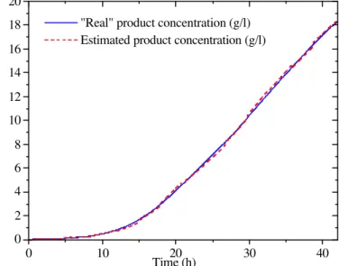
a)Unfaulty Fermentation

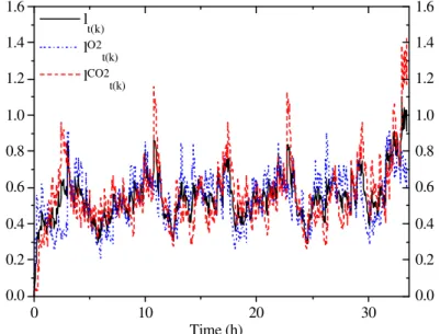
To observe the behavior of the estimation-detection methodology, an unfaulty case is presented. Initial conditions and stochastic parameters used to simulate this run are presented in Table 4. Fig. 3 shows the evolution of indicators lt(k), lO2t(k) and lCO2t(k)

and Table 5 shows the evolution of indicators ht(k),

hi

t(k) and h-it(k) for this case. These indicators were

compared to their thresholds for detection tests and no faults were detected. Thus, estimated states are assumed to be correct. They can be compared with ‘real’ states in Figs. 4. Note that, in spite of errors in some stoichiometric yields and uncertainty in the kinetic parameters, an excellent agreement between estimated and real state variables was obtained.

Table 4: Initial conditions and stochastic parameters used to simulate the unfaulty fermentation

"Real" initial concentrations: X0 = 0.0133 g/l, S0 = 25.045 g/l.

Stochastic parameters P/O = 1.298, δp = 0.41, kS = 1.066 g S/l

YX/N = 7.88 g X/g N, kATPm = 0.589 mol ATP/g X h

Stoichiometric yields

YX/S = 1.741 g X/g S, YX/CO2 = 12.335

g X/g CO2, YP/S = 0.9121 g P/g S

YP/CO2 = 32.99 g P/g CO2, YP/O2 = 15.45 g P/g O2

YNADH2/P = 3.67 mol ATP/g P

Kinetic disturbances

∆µM 0 = -0.036 h-1, ∆XS 0 = 0.155 g X/l

∆a0 = -0.541 g P/g X, ∆b0 = 0.0113 g P/g X h

∆µM u = -0.0004 h-1/°C, ∆XS u = -0.0070 g X/l°C

∆au = 0.130 g P/g X°C, ∆bu = 0.0031 g P/g X h°C

10 20 30 40

0.0 0.2 0.4 0.6 0.8 1.0 1.2

0.0 0.2 0.4 0.6 0.8 1.0 1.2 l

t(k)

lO2 t(k)

lCO2 t(k)

Time (h)

Table 5: Evolution of indicators ht(k), h i

t(k) and h i

t(k) for the unfaulty run

t(k) ht(k) hO2t(k) hCO2t(k) hSt(k) hXt(k) hPt(k) h-O2t(k) h-CO2t(k) h-St(k) h-Xt(k) h-Pt(k)

2.76 5.76 8.76 11.76 14.76 17.76 20.76 23.76 26.76 29.76 32.76 35.76 38.76 41.76

3.794 3.401 0.015 1.100 4.627 0.709 0.310 0.278 4.029 1.631 1.044 0.038 3.712 2.610

0.477 0.416 0.002 0.270 1.679 0.483 0.055 0.089 2.301 0.782 0.148 0.031 2.630 0.967

1.468 2.307 0.006 0.295 2.664 0.006 0.103 0.057 1.706 0.159 0.385 0.002 1.065 0.440

1.563 0.58 0.006 0.452 0.247 0.184 0.129 0.111 0.020 0.581 0.432 0.004 0.013 1.014

0.176 0.055 0.001 0.052 0.019 0.023 0.015 0.013 0.000 0.070 0.049 0.001 0.005 0.120

0.109 0.043 0.000 0.031 0.019 0.012 0.009 0.008 0.002 0.039 0.030 0.000 0.000 0.069

3.316 2.984 0.013 0.830 2.949 0.226 0.255 0.189 1.728 0.850 0.896 0.007 1.083 1.643

2.325 1.094 0.009 0.806 1.963 0.702 0.207 0.220 2.323 1.472 0.659 0.036 2.648 2.171

2.230 2.821 0.009 0.648 4.380 0.525 0.182 0.167 4.009 1.051 0.612 0.034 3.699 1.596

3.618 3.345 0.014 1.048 4.608 0.685 0.296 0.265 4.029 1.562 0.995 0.037 3.708 2.491

3.685 3.358 0.014 1.069 4.608 0.696 0.301 0.270 4.027 1.592 1.014 0.038 3.712 2.541

0 10 20 30 40

0.0 0.5 1.0 1.5 2.0

Time (h)

"Real" biomass concentration (g/l) Estimated biomass concentration (g/l) "Real" quantity of oxidized main substrate (g/l) Estimated quantity of oxidized main substrate (g/l)

Figure 4.a: Real and estimated values of states X and SR for the unfaulty run

0 10 20 30 40

0 2 4 6 8 10 12 14 16 18 20

"Real" product concentration (g/l) Estimated product concentration (g/l)

Time (h)

b) Faulty Scenarios

Test cases are presented below to demonstrate the ability of the estimation-detection program to identify an unexpected event and its characteristic parameters. In these tests, the stochastic model was started with the parameters in Table 4 under normal operating conditions and the states were propagated before a given bias was imposed at a given occurrence time. Fault parameters are summarized in Table 6. The tests always detected the occurrence of a fault, reflecting the increased detection power arising from multiple tests as can be seen in Table 7 and Figs. 5 to 7. Fault isolation is achieved by hypothesizing alternative sources and by using the maximum likelihood identification procedure in a ten-hour time window (the six hours previous to the alarm launch plus four hours from the alarm launch for collection of dynamic information). The identification is to estimate faulty parameters and log-likelihood functions for each alternative. The capability of the technique to distinguish between

alternative hypotheses is reflected by the results in Table 8. The first table compares the term Σt(j)=t0t(j)=t(k)

[(yt(j) – cIJ(x,υ,τ)) V-1t(j) (yt(j) – cIJ(x,υ,τ))T] of the

likelihood function (19) for each hypothesis (I,J). This is the critical term in eq. (19), since Σt(j)=t0t(j)=t(k)

lnVt(j) was almost constant. The second table

compares Σt(j)=t0t(j)=t(k) (ht(k)) for all hypotheses. Note

that this summation provides useful information for further discriminating between different hypotheses. Log-likelihood values for many hypotheses are rather similar, indicating similarity of dynamics for different error sources. Furthermore, as can be expected, measurement faults are clearly easier to distinguish than incorrect system descriptions. Nevertheless, the true hypothesis was correctly selected in most cases, even with high noise and parametric uncertainty. Estimated faulty parameters are shown in Table 9. They can be compared with true fault parameters presented in Table 6. The results show that faulty parameters can be estimated with fairly good precision.

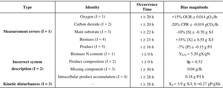
Table 6: Fault parameters for simulated faulty runs

Type Identity Occurrence

Time Bias magnitude

Oxygen (J = 1) t ≥ 20 h +15% OUR.≅ 0.014 gO2/lh

Carbon dioxide (J = 2) t ≥ 20 h -20% CPR ≅ -0.019 gCO2/lh

Main substrate (J = 3) t ≥ 22 h -10% [S] ≅ -0.70 g S/l

Biomass (J = 4) t ≥ 23 h +35% [X] ≅ 0.55 g X/l

Measurement errors (I = 1)

Product (J = 5) t ≥ 16 h -7% [P] ≅ -0.15 g P/l

Biomass N-content (J = 1) t ≥ 0 h YX/N = 5.20 gX/gN

Product composition (J = 2) t ≥ 0 h δp = 0.52

Missing component (J = 3) t ≥ 30 h 0.04 g/lh

Incorrect system

description (I = 2)

Intracellular product accumulation (J = 4) t ≥ 28 h 0.18 g P/l h

Kinetic disturbances (I = 3) - t ≥ 28 h XS = 3.9 g X/l; b =0.27 gP/gXh

Table 7: Evolution of indicators ht(k), h

i

t(k) and h i

t(k) for faulty runs

t(k) ht(k) hO2t(k) hCO2t(k) hSt(k) hXt(k) hPt(k) h-O2t(k) h-CO2t(k) h-St(k) h-Xt(k) h-Pt(k)

(I = 1, J = 3)

2.76 5.76 8.76 11.76 14.76 17.76 20.76 23.76

3.794 3.401 0.015 1.1 4.627 0.709 0.31 105.59

0.477 0.416 0.002 0.27 1.679 0.483 0.055 20.581

1.468 2.307 0.006 0.295 2.664 0.006 0.103 33.233

1.563 0.58 0.006 0.452 0.247 0.184 0.129 43.761

0.176 0.055 1E-3 0.052 0.019 0.023 0.015 4.991

0.109 0.043

0 0.031 0.019 0.012 0.009 3.03

3.316 2.984 0.013 0.83 2.949 0.226 0.255 85.016

2.325 1.094 0.009 0.806 1.963 0.702 0.207 72.364

2.23 2.821 0.009 0.648 4.38 0.525 0.182 61.836

3.618 3.345 0.014 1.048 4.608 0.685 0.296 100.60

Continuation Table 7

(I = 1, J = 4)

2.76 5.76 8.76 11.76 14.76 17.76 20.76 23.76 26.76 3.794 3.401 0.015 1.1 4.627 0.709 0.31 5.042 6.56 0.477 0.416 0.002 0.27 1.679 0.483 0.055 2.016 0.03 1.468 2.307 0.006 0.295 2.664 0.006 0.103 0.746 4.217 1.563 0.58 0.006 0.452 0.247 0.184 0.129 1.921 1.968 0.176 0.055 1E-3 0.052 0.019 0.023 0.015 0.228 0.204 0.109 0.043 0 0.031 0.019 0.012 0.009 0.131 0.141 3.316 2.984 0.013 0.83 2.949 0.226 0.255 3.026 6.53 2.325 1.094 0.009 0.806 1.963 0.702 0.207 4.296 2.342 2.23 2.821 0.009 0.648 4.38 0.525 0.182 3.121 4.592 3.618 3.345 0.014 1.048 4.608 0.685 0.296 4.815 6.355 3.685 3.358 0.014 1.069 4.608 0.696 0.301 4.911 6.419

(I = 1, J = 5)

2.76 5.76 8.76 11.76 14.76 17.76 20.76 23.76 3.794 3.401 2.437 2.469 0.616 0.115 1.276 16.681 0.477 0.416 0.002 0.617 0.058 1E-3 0.25 1.621 1.468 2.307 1.472 0.652 0.42 0.066 0.4 7.025 1.563 0.58 0.819 1.013 0.118 0.041 0.529 6.802 0.176 0.055 0.087 0.117 0.011 0.004 0.06 0.758 0.109 0.043 0.058 0.07 0.009 0.003 0.037 0.475 3.316 2.984 2.436 1.852 0.559 0.114 1.026 15.06 2.325 1.094 0.965 1.817 0.196 0.049 0.876 9.656 2.23 2.821 1.619 1.456 0.498 0.074 0.747 9.879 3.618 3.345 2.351 2.352 0.605 0.11 1.216 15.922 3.685 3.358 2.379 2.399 0.608 0.112 1.24 16.206

(I = 2, J = 1)

2.76 5.76 8.76 11.76 14.76 17.76 3.647 3.159 0.203 0.101 5.248 10.133 0.45 0.509 0.047 0.019 4.185 3.839 1.422 2.114 0.057 0.032 0.842 1.648 1.502 0.46 0.084 0.042 0.179 3.917 0.169 0.043 0.01 0.005 0.031 0.462 0.105 0.034 0.006 0.003 0.01 0.268 3.198 2.651 0.156 0.082 1.063 6.295 2.225 1.045 0.146 0.069 4.406 8.486 2.145 2.7 0.119 0.059 5.069 6.216 3.479 3.117 0.193 0.096 5.217 9.671 3.543 3.125 0.197 0.098 5.238 9.865

(I = 2, J = 2)

2.76 5.76 8.76 11.76 14.76 17.76 20.76 23.76 26.76 29.76 32.76 35.76 38.76 41.76 3.779 3.364 0.024 0.955 4.283 1.091 0.991 0.063 3.636 4.732 4.932 1.852 5.489 10.807 0.476 0.42 0.003 0.252 1.775 0.579 0.115 0.023 2.908 1.254 0.448 0.024 3.991 1.959 1.462 2.28 0.01 0.241 2.325 0.075 0.394 0.036 0.568 1.188 2.116 1.032 0.005 3.546 1.558 0.568 0.01 0.391 0.159 0.367 0.407 0.003 0.130 1.934 2.005 0.675 1.249 4.482 0.175 0.054 1E-3 0.045 0.011 0.045 0.046 0.000 0.022 0.223 0.223 0.073 0.161 0.51 0.108 0.042 1E-3 0.027 0.013 0.025 0.028 0.000 0.008 0.133 0.14 0.048 0.083 0.311 3.303 2.943 0.021 0.703 2.508 0.512 0.875 0.040 0.728 3.478 4.484 1.828 1.498 8.848 2.317 1.083 0.014 0.715 1.958 1.016 0.597 0.027 3.068 3.544 2.816 0.819 5.484 7.261 2.222 2.796 0.014 0.565 4.123 0.724 0.584 0.059 3.506 2.799 2.928 1.176 4.240 6.325 3.604 3.31 0.023 0.91 4.272 1.047 0.945 0.062 3.613 4.509 4.709 1.779 5.328 10.297 3.671 3.322 0.023 0.929 4.27 1.067 0.962 0.062 3.628 4.599 4.792 1.804 5.406 10.496

(I = 2, J = 3)

2.76 5.76 8.76 11.76 14.76 17.76 20.76 23.76 26.76 29.76 32.76 3.794 3.401 0.015 1.1 4.627 0.709 0.31 0.278 4.029 2.609 6.301 0.477 0.416 0.002 0.27 1.679 0.483 0.055 0.089 2.301 1.024 0.806 1.468 2.307 0.006 0.295 2.664 0.006 0.103 0.057 1.706 0.399 2.423 1.563 0.580 0.006 0.452 0.247 0.184 0.129 0.111 0.02 0.999 2.598 0.176 0.055 0.001 0.052 0.019 0.023 0.015 0.013 0.000 0.118 0.292 0.109 0.043 0.000 0.031 0.019 0.012 0.009 0.008 0.002 0.068 0.181 3.316 2.984 0.013 0.83 2.949 0.226 0.255 0.189 1.728 1.585 5.494 2.325 1.094 0.009 0.806 1.963 0.702 0.207 0.220 2.323 2.209 3.877 2.230 2.821 0.009 0.648 4.380 0.525 0.182 0.167 4.009 1.610 3.702 3.618 3.345 0.014 1.048 4.608 0.685 0.296 0.265 4.029 2.491 6.009 3.685 3.358 0.014 1.069 4.608 0.696 0.301 0.27 4.027 2.54 6.12

(I = 2, J = 4)

10 20 0.0

0.2 0.4 0.6 0.8 1.0 1.2 1.4

0.0 0.2 0.4 0.6 0.8 1.0 1.2 1.4 l

t(k)

lO2 t(k)

lCO2 t(k)

Time (h)

Figure 5: Evolution of indicators lt(k), lO2t(k) and lCO2t(k) for the case of a bias in the O2 measurement

10 20

0.0 0.2 0.4 0.6 0.8 1.0 1.2 1.4 1.6

0.0 0.2 0.4 0.6 0.8 1.0 1.2 1.4 1.6 l

t(k)

lO2 t(k)

lCO2 t(k)

Time (h)

Figure 6: Evolution of indicators lt(k), lO2t(k) and lCO2t(k) for the case of a bias in the CO2 measurement

0 10 20 30

0.0 0.2 0.4 0.6 0.8 1.0 1.2 1.4 1.6

0.0 0.2 0.4 0.6 0.8 1.0 1.2 1.4 1.6 l

t(k)

lO2 t(k)

lCO2 t(k)

Time (h)

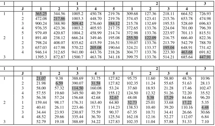
Tables 8: Hypothesis discriminability. The columns in the first table show a comparison of the term Σt(j)=t0

t(j)=t(k)

[(yt(j) – cIJ(x,υ,τ)) V -1

t(j) (yt(j) – cIJ(x,υ,τ)) T

] of the log-likelihood function (16) of all hypotheses (I,J). Columns in the second table show a comparison

of Σ (ht(k)) of all hypotheses. (Grey boxes denote the most probable fault)

I 1 2 3

J 1 2 3 4 5 1 2 3 4

1 1 365.25 344.56 1005.2 450.78 219.76 309.68 127.36 218.11 664.52 726.93

2 472.08 217.86 1003.3 448.70 219.76 374.45 123.41 215.76 653.78 474.98

3 900.24 388.90 509.42 276.60 184.12 215.78 132.69 195.53 528.69 696.83

4 976.35 423.36 1003.2 405.93 217.75 372.65 133.76 224.04 701.00 796.39

5 979.49 420.87 1004.2 458.99 214.74 372.98 133.76 223.97 701.13 815.51

2 1 891.40 238.12 666.24 349.46 195.08 255.50 122.09 216.75 666.40 822.36

2 798.24 408.07 835.62 415.59 216.51 339.07 133.76 213.79 542.79 788.70

3 657.03 417.98 570.22 205.08 190.64 324.21 133.37 195.04 648.91 731.42

4 946.14 312.65 941.00 443.76 218.26 304.77 133.76 223.30 463.68 691.82

3 1395.3 872.87 1500.7 463.78 341.18 399.75 133.76 514.21 685.64 447.91

I 1 2 3

J 1 2 3 4 5 1 2 3 4

1 1 21.07 9.38 388.69 31.75 127.82 95.75 11.60 58.80 48.76 10.96

2 21.98 6.59 390.07 31.58 127.82 102.35 11.24 55.65 51.63 28.13

3 58.00 57.32 114.50 160.08 53.24 37.60 18.93 21.28 17.46 102.47

4 57.55 19.60 349.50 40.39 155.12 124.50 12.32 51.26 72.20 35.52

5 56.38 57.24 156.68 42.68 32.67 48.08 5.38 17.29 84.66 96.20

2 1 159.44 98.17 176.31 163.40 64.80 32.73 25.01 33.68 17.22 5.35

2 40.41 26.11 223.46 37.71 114.23 138.53 10.40 39.20 110.16 4.48

3 34.44 23.93 230.87 75.59 90.37 67.35 10.71 34.41 26.66 30.66

4 48.52 29.66 335.44 36.70 125.54 162.18 12.16 52.27 112.07 6.84

3 52.79 19.18 388.69 34.22 127.83 102.35 11.04 57.88 51.33 7.10

Table 9: Detection and diagnosis results for faults in Table 6.

I _τ∧ _υ∧ Detection

time

Alarm launcher J

1 1 21.75 h 0.02 g O2 /l h 25.00 h lt(k)O2

2 21.75 h -0.025 g CO2/l h 22.75 h lt(k)CO2

3 17.75 h -0.60 g S/l 23.75 h ht(k)

4 20.75 h 0. 60 g X/l 26.75 h ht(k)

5 20.75 h -0.30 g P/l 23.75 h ht(k)

2 1 <11.75 h 7.50 g X/g N 17.75 h ht(k)

2 40.75 h 0.40 41.75 h ht(k)

3 26.75 h 0.05 g/l h 32.75 h ht(k)

4 29.75 h 0.035 g P/l h 35.75 h ht(k)

3 31.75 h XS = 2.8 g X/l 33.52 h lt(k) CO2

c) Estimation of Measurement Variances

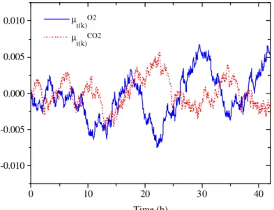
In Figures 8 and 9 estimated means and variances of measurement residuals for the run in section 4.2.1 are plotted. They were calculated in a w’ = 75-sample lag-time window for on-line measurements and w’ = 5-sample lag-time window for off-line measurements. Note that a relatively accurate prediction of on-line measurement variances can be obtained. For off-line measurements, the estimated variances are not very accurate.

0 10 20 30 40 -0.010

-0.005 0.000 0.005 0.010

Time (h) µ_t(k)O2

µ

t(k)CO2

Figure 8.a: Estimated residual means of O2 and CO2 measurements for the unfaulty run

15 20 25 30 35 40

-0.02 0.00 0.02 0.04 0.06 0.08 0.10 0.12

Time (h)

µ

S2

µ

X2

µ_P2

Figure 8.b: Estimated residual means of S, X and P measurements for the unfaulty run

10 20 30 40

0.0000 0.0004 0.0008 0.0012

Time (h) σ

t(k)O2

σ

t(k)CO2

15 20 25 30 35 40 0.01

0.02 0.03 0.04

Time (h)

σ_S2

σ_X2

σ

P2

Figure 9.b: Estimated residual variances of S, X and P measurements for the unfaulty run

CONCLUSIONS

An approach to estimate state and parameters and to isolate unexpected events in batch fermentations with nonlinear and uncertain dynamics was developed. It is based on the application of several statistical detection tests and maximum likelihood state and parameter estimation techniques. The approach is designed for faulty structure discrimination. A maximum likelihood filter is used to identify faults. For computational efficiency, the fault parameters are estimated in a fixed-size sliding window. Under null hypothesis, the outputs of the algorithm are the fermentation state and parameter values. Under fault hypothesis, the outputs are states, maximum-likelihood fault parameters and log-likelihood function values. These values are used for statistical comparison with the alternative faulty hypothesis. The original contributions of the method are

§ The application of multiple tests, including

measurement-dedicated detection tests of the residuals of the monitor filter and balance equations.

§ The on-line implementation of

maximum-likelihood state and parameter estimation within the detection procedure for both the unfaulty process model and faulty models using a robust (Jacobian-free and Hessian-(Jacobian-free) optimization method.

The technique was illustrated for simulated xanthan gum batch fermentations and ten different faulty scenarios were simulated. In spite of nonlinearities, parametric uncertainty and kinetic

variations, hypothesis discriminability was very good.

Areas of continuing work include the application and development of data-fusion techniques to fuse data from tests with maximum-likelihood estimates for gaining computational efficiency and hypothesis discriminability in small sample data. Research on the use of the algorithm in multiple -faults tests and in real fermentations is also advisable.

NOMENCLATURE

ϕ Critical threshold of statistical indicator l ϕI _{Critical threshold of statistical indicator l}i

ϕ--i _{Critical threshold of statistical indicator l}-i

θ Critical threshold of statistical indicator h θ i _{Critical threshold of statistical indicator h}i

θ--I _{Critical threshold of statistical indicator h}-i

∆µ Disturbance of the specific biomass growth (h-1₎

∆a Disturbance of the growth-associated

specific metabolite production (g P/g X)

∆b Disturbance of the steady specific

metabolite production (g P /g X h)

∆CO2 Cumulative carbon dioxide production (g

CO2/l)

∆KR _{Disturbance of the specific substrate}