www.scielo.br/rbg
SEISMIC RAY TOMOGRAPHY USING
L
1INTEGRAL NORM
Vˆania G. de Brito dos Santos
1and Wilson M. Figueir´o
2Recebido em 23 dezembro, 2008 / Aceito em 28 junho, 2011 Received on December 23, 2008 / Accepted on June 28, 2011
ABSTRACT.Seismic ray tomography methods are usually associated with substantial computer processing time. The reason for this is that at each step of the iterative inversion process defined by the tomographic method the two-point ray tracing problem must be solved for each source-receiver pair. In order to resolve this, an Euclidean norm (L2vector norm), commonly used in error functions which are to be minimized in inversion procedures, is substituted by anL1integral norm, which enables the estimation of model parameters by minimizing the area between observed and calculated traveltime curves that are interpolated (or adjusted) to the data points. Relatively simple mathematical developments and numerical experiments with two-dimensional compressional seismic wave velocity field models show thatL1integral norm saves an enormous amount of processing time with no significant loss of accuracy. Occasionally, parameters of the model can be better estimated usingL1integral norm than theL2vector norm that is traditionally utilized in seismic inversion tomography.
Keywords: seismic ray, tomography, polynomial parameterization, seismic velocity field, two-point ray tracing problem,L2vector norm,L1integral norm.
RESUMO.O alto consumo de tempo em processamento computacional ´e um problema que, geralmente, est´a associado aos m´etodos de tomografia s´ısmica. Isto ocorre porque, em cada passo do processo iterativo de invers˜ao definido pelo m´etodo tomogr´afico, o problema da conex˜ao de dois pontos, pela curva da trajet´oria do raio s´ısmico, deve ser resolvido para cada par fonte-receptor. A fim de reduzir a gravidade deste tipo de problema, a norma Euclideana (normaL2 de vetor), comumente empregada nas func¸˜oes de erro a ser minimizado no processo de invers˜ao, ´e substitu´ıda por uma normaL1de func¸˜ao. Essa mudanc¸a permite estimar parˆametros do modelo atrav´es da minimizac¸˜ao da ´area entre curvas de tempos observados e calculados que s˜ao interpoladas (ou ajustadas) aos pontos referentes aos dados. Desenvolvimentos matem´aticos e experimentos num´ericos relativamente simples, com modelos bidimensionais de campos de velocidade s´ısmica de ondas compressionais, mostram que a normaL1de func¸˜ao permite poupar uma enorme quantidade de tempo de processamento sem uma importante perda de precis˜ao. `As vezes, os parˆametros do modelo s˜ao estimados de modo mais acurado usando-se a normaL1da integral em lugar da normaL2de vetor, tradicionalmente usada na invers˜ao tomogr´afica.
Palavras-chave: raio s´ısmico, tomografia, parametrizac¸˜ao polinomial, campo de velocidade s´ısmica, problema de conex˜ao de dois pontos por trac¸ado de raio, normaL2de vetor, normaL1de integral.
1Universidade Estadual de Feira de Santana, Departamento de Ciˆencias Exatas, m´odulo V, Km 3, BR-116, Campus Universit´ario, s/n, Caixa Postal 252294, 44031-460 Feira de Santana, BA, Brazil. Phone: +55 (75) 3161-8086 – E-mail: vania [email protected]
INTRODUCTION
The concept of distance between observed and calculated data has a central role in inverse geophysical problems, where it can be expressed in terms of norms. Over the years certain works have attempted to improve objective functions based on norms, with improvements being witnessed in respect of the following issues: robustness, regularization, stability, accuracy, and pro-cessing time reduction. Claerbout & Muir (1973) suggested that some norms are more appropriate than others depending on the application, for example: the L1-norm is more robust than the
L2-norm. Scales & Gersztenkorn (1988) presented an alternative
to the regularization of inverse problems based on theL1-norm
(least-absolute deviation) instead of damped least squares. Bube & Langan (1997) applied iteratively re-weighted least square to a hybridL1/L2minimization problem that works better for data
with outliers than theL2algorithm with a small additional
com-putational cost. A combination of the L2-norm withL1-norm
has been established by the so-called Huber norm that gives us more robust parameter model estimation than the L2-norm and
it retains its smoothness better than theL1-norm for small
resid-uals (Guitton & Symes, 2003). When wavelets are used to rep-resent models, theL1-norm is better thanL2regularization on
wavelet decomposition used to represent a model solution of a linearized seismic tomographic problem (Loris et al., 2007). Dif-ferent norms are compared and used in combination with nonlin-ear regularization techniques in order to discuss seismic tomo-graphy aspects such as: ill-conditioned matrices, model recon-struction, and time-consumption (Loris et al., 2010).
Amongst other issues, seismic ray tomography is faced with the problem of large amounts of processing time being wasted in order to estimate model parameters. The traditional objective functions (Bishop et al., 1985) that useL2vector norm, need to
have a time calculated at the same receiver where a seismic ray arrives and where a real traveltime is observed. This means that for each source-receiver pair, the two-point ray tracing problem must be solved. The problem is therefore accentuated because, with tomographic work, it is recommended to have a good cover-age of the velocity field model, and so it is necessary to have a large number of source-receiver pairs connected by seismic ray trajectories, for which traveltimes are calculated. In addition, even for relatively simple two-dimensional models, the two-point ray tracing problem is an iterative process that can result in pro-longed computer processing time. Given that seismic tomo-graphy is also an iterative method, the same procedure of con-necting source and receiver positions (for each one of the
sev-eral source-receiver pairs) must be repeated to this extent, since this is the supposed number of required iterations for conver-gence. In order to mitigate against such a worrying problem, we propose a substitution of the traditional L2vector norm by an
alternative integral L1-norm that does not demand connection
positions by ray trajectories and, consequently, saves a signific-ant amount of processing time.
Seismic Ray Tracing and Traveltime Calculation
IfV(x,z)is a two-dimensional velocity field model,T repres-ents traveltime, anddsis an arc length element; then to find the trajectoryCthat minimizes the functional
T(C)=
Z
C ds
V(x,z), (1)
requires that the following system of equations be solved ( ˇCerven´y, 1987)
dx(τ )
dτ =p(τ )
dp(τ )
dτ =
1
2
E ∇ 1
V2
(x,z)
,
(2)
whereτis a ray parameter,x(τ )is a vector position of a ray tra-jectory point atτ andp(τ )is the slowness vector that is tangent to the ray trajectory atτ. Numerically, rays are traced by means of the following recursive system
x(τ+1τ )=x(τ )+p(τ )1τ
p(τ+1τ )=p(τ )+1
2
E
∇h 1
V2
(x(τ ),z(τ )) i
1τ ,
(3)
obtained by a Taylor expansion of Equation (2). In this work, the two-point ray tracing problem is solved by the Heun method (Santos & Figueir´o, 2006). The traveltime along ray trajectory is calculated numerically by the following expression:
T(xN+1,zN+1) =
N
X
i=0 1Ti
= N
X
i=0
1
Vi ∙ kxi+1−xik2, (4)
where the calculation of the traveltime element, 1Ti at each knot of the polygonal line, which represents the ray trajectory, is achieved concomitantly with its trace;Vi is the wave velocity at the pointxi = (xi,zi); N +1is the total number of small straight segments that constitute the ray trajectory up toxN+1;
andk k2is the Euclidean norm. At the end of each step in the
must be up-to-date in order to satisfy the eikonal equation in the following way:
kpk2= q
p12+p 2 2=
1
V(x,z), (5)
wherep = (p1,p2)with p1 = kpk2 ∙ cos(θ ), p2 = kpk2∙sin(θ )andθis the departure angle, meaning the angle
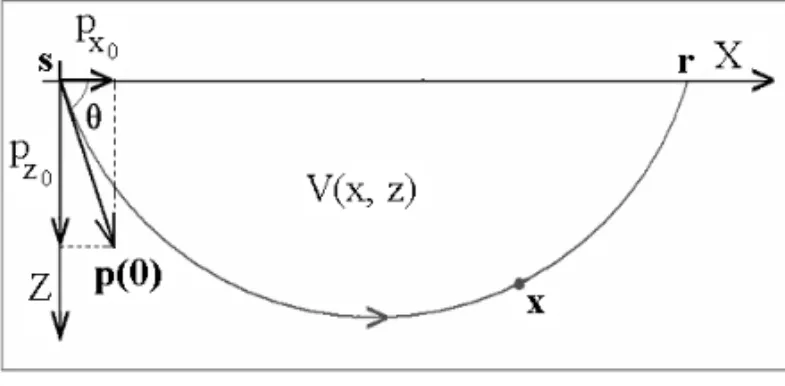
between p(0)and the positive orientation of the X axis, see Figure 1. In other words, the direction ofpis preserved, but its magnitude is altered in order to satisfy Equation (5). Initial con-ditions necessary to solve the ray tracing equations are: source positions =(x = 0,z =0)= 0and the slowness vector, p(0)given by 1
V(0,0)(cos(θ ),sin(θ )).
Figure 1– Illustration of a ray trajectory between the sourcesand the receiver
rshowing vectorsxandp(the latter has axis projectionspx0andpz0). In the iterative process performed in order to solve the two-point ray tracing problem that connects source to receiver, the bisection method is used to determine the departure angleθ of the ray trajectory. Figure 2 shows a ray network obtained by em-ploying numerical methods such as those presented here for the seismic velocity target modelV2used for inversions in this work.
Figure 2– A ray network on the velocity field model expressed by Equation (29). Within it, the two-point ray tracing problem is solved for each source-receiver pair.
Gauss-Newton Method
The solution of an inverse problem begins with the use of a set of observed data (real or synthetic), and can be divided into three
steps: model parameterization, direct modeling, and inverse modeling (Figueir´o, 1994). The latter consists of the determina-tion (or estimadetermina-tion) of model parameters that employ the afore-mentioned data set. The local optimization method called Gauss-Newton is an iterative procedure that enables us to solve a non-linear problem by means of successive non-linearization. In fact, the problem is solved on a step-by-step basis by applying, repeatedly, the least squares method.
In the modeling process the input of the system is described by model vectormwhose components are the model parameters. As the problem is linearized, the output, in forward modeling, can be expressed byGmwhereGis a matrix that describes the wave propagation process that depends on the geometrical struc-ture of the problem. The modelmcan be written as:
m=(m1,m2,m3, . . . ,mm)T. (6)
If the vectord=(d1,d2,d3, . . . ,dn)T contains the observed
data (synthetic for the purpose of this work, but it can be real, if available), then in order to solve the inverse problem we need to find the modelmthat minimizes the following residual error function:
e(m)=d−Gm. (7)
A candidate for a minimum of Equation (7) is a least squares solution for the objective function8(m)written as follows:
8(m)=e(m)Te(m)=(d−Gm)T(d−Gm) . (8)
The so-called least square solution of Equation (8) is provided by (Menke, 1989):
m=(GTG)−1GTd. (9)
And residual error function is given by
1d(m)=dobs−dcalc(m) , (10)
wheredobs anddcalc(m)are, respectively, the observed data and the calculated data for the modelm. If1dis nonlinear, it can become linear using its first order Taylor series expansion. It produces:
1dap(m)=1d(m0)+S(m0)1m, (11)
where1dap is the linear approximation of1d,m0is a
refer-ence model (not necessarily an initial one, but more appropriately a current model),1m=m−m0is a model perturbation, and S(mk)is the sensibility matrix calculated at the current model mk. The ij-th entry ofS(mk)is provided by:
Si j(mk)=
∂dcalc,i
∂mj
The solution of Equation (11) is then:
1mk=
h
S(mk)TS(mk)
i−1
S(mk)T1d(mk) . (13)
This enables the following iterative procedure:
mk+1=mk+1mk. (14)
In this exposed way, the inverse iterative process employing an L2vector norm is characterized.
Iterative Process defined by theL1Integral Norm
Letmt = (μ1, μ2, μ3, . . . , μm)T be a target model, where m is its number of parameters. All the parameters ofmt are fixed and unknown. For mt we have n pairs of data(xi,ti) wheretiis the synthetic observed traveltime data for the receiver positionxi.
Then, we can construct a polynomial function,
tobs(x)=a0+a1x+a2x 2
+ ∙ ∙ ∙ +apxp, (15)
by means of cubic spline interpolation (Santos, 2009) using pairs
(xi,ti),i =1,2, . . . ,18,xi ∈ I = [0,xmax], obtained by
the ray-tracing method. The SPLINE((xi,ti),x)MATLAB rou-tine was used to generate a piecewise third degree polynomial S3(x), i.e. a cubic spline on the interval I. After that,S3(x)is
sampled in the pointsxk =k∙10−2,k =0,1,2, . . . ,900,
in order to use POLYFIT(xk,S3(xk),p)MATLAB routine,
pro-ducing a polynomial of degree p = 8 by adjustment to the
data(xk,S3(xk)). Such a choice was motivated by the need to
have a sufficient degree of freedom and not so much oscillation in agreement with the synthetic observed data behavior.
Ifm = (η1, η2, η3, . . . , ηm)T represents a general (or a current) model that can vary freely and produces n pairs
(xi˜,ti˜)of calculated traveltimes,ti˜ at the arrival position,xi˜ of a seismic ray; then we can obtain (applying the same procedure used to obtain Equation (15)), a polynomial function
tcalc[m](x)=b0+b1x+b2x2+ ∙ ∙ ∙ +bqxq, (16)
where[m]is to remind us that the calculated traveltime depends onm. These two kinds of data pairs (observed and calculated) and the two functionstobs(x)andtcalc[m](x)are represented in
Figure 3.
The problem consists in to find a modelm that minimizes the area function
A(m) = ktobs(x)−tcalc[m](x)ki nt
=
Z xmax
0
tobs(x)−tcalc[m](x)
d x,
(17)
whereA(m)is a non-negative scalar functional defined inRm. It is supposed that the modelmk+1is produced by a
perturba-tion1mk, i.e.,mk+1 = mk +1mk. Then, A(mk+1) =
A(mk +1mk). Using a Taylor expansion of A(mk+1), we
have:
A(mk+1) = A(mk)+ E∇A(mk)1mk
+1
21m
T
kH(mk)1mk+ ∙ ∙ ∙, (18)
where
E
∇A(mk) =
∂A
∂η(mk)
= gk
∂
A
∂η1 ,∂A
∂η2
, . . . , ∂A ∂ηm
(mk) (19)
and
H(mk)= ∂2A
∂η2(mk)
=
∂2A
∂η12
∂2A
∂η1∂η2 . . .
∂2A
∂η1∂ηm
∂2A
∂η2∂η1
∂2A
∂η22
. . . ∂
2 A
∂η2∂ηm .
.
. ... ...
∂2A
∂ηm∂η1
∂2A
∂ηm∂η2 . . .
∂2A
∂η2 m
(mk) (20)
is the Hessian matrix.
As we expectA(mk+1)to assume a minimum (in fact, the
desired value of the minimum we are seeking is zero, as can be seen in (17)), we can make its linear approximation, the two first terms of Equation (18), equal to zero, and so:
1mk= −(gTkgk)−
1
gTk A(mk) (21)
defines an iterative process. The partial derivative ∂η∂A1(m)
is a real number and is calculated numerically by means of the expression:
A(. . . , ηi+1ηi, . . .)−A(. . . , ηi, . . .)
1ηi
,
where1ηi is a small perturbation of the parameterηi. It quan-tifies the variation of the area between the curves tcalc[m](x)
andtobs(x)when the model parameterηiis perturbed.
Some Special Comments
To obtain ∂A
∂ηi(m)which is a component of the vectorgk it is necessary to calculate A(m). This is done by means of the ABS and INT MATLAB routines. However, it is important to say that it is possible to obtain an analytical expression for A(m)
and, for the sake of illustration, it is obtained as follows: initially, we have1T[m](x) = tobs(x)−tcalc[m](x). Without loss
of generality, we can consider the polynomials (15) and (16) to the same degree, i.e., p = q andxmax > 0. Let us
con-siderr1,r2,r3, . . . ,ru(u ≤ p)the real roots of1T[m](x),
where its sign change, and, for the sake of uniformity,r0 = 0
andru+1 = xmax (it is possible to choose adjusted
poly-nomials tobs(x) and tcalc[m](x), such that 0 and xmax are
not roots of1T[m](x)).
Then,
A(m) =
Z xmax
0
1T[m](x)d x
= u
X
i=0 Z ri+1
ri
sgn1T[m](x)
1T[m](x)d x.
(22)
This implies:
A(m)=sgn1T[m](0)
× u
X
i=0 (−1)i
Z ri+1
ri p
X
j=0
(aj−bj)xjd x
(23)
and finally
A(m)=sgn
1T[m](0)
× u
X
i=0 (−1)i
p
X
j=0
(aj−bj) j+1
rij++11−r
j+1
i
.
(24)
It is interesting to observe that
A(m) =
Z xmax
0
1T[m](x)
d x
≤ p
X
i=0 Z xmax
0 ai−bi
xid x
= p
X
i=0
xmaxi+1
i+1
ai−bi
(25)
and if the polynomial coefficients oftobs and tcalc[m](x)are
obtained satisfying the inequality constraint
7 X
j=0 8 X
k=j+1
xmaxi+k+2
we have: v u u t 8 X
i=0
(ai−bi)2≤ v u u u t 8 X
i=0 "
xmaxi+1
i+1(ai−bi)
#2 ≤ v u u u t 8 X
i=0 "
xmaxi+1
i+1(ai−bi)
#2 = 8 X
i=0
xmaxi+1
i+1(ai−bi)
= xmax Z 0 8 X
i=0
(ai−bi)xid x ≤ xmax Z 0
1T[m](x)d x
=A(m) .
(27)
Equations (25) and (27) shows thatA(m)is between theL2
vector norm and anL1vector pondered norm, where the vectors a = (a0,a1, . . . ,a8)andb = (b0,b1, . . . ,b8)are
com-posed of the polynomial coefficients oftobs(x)andtcalc[m](x)
withbi dependent of the model parameters, respectively. There-fore, it represents an intermediary norm that has the robustness and smoothness (near the minimum) that lack to theL2vector
norm (in case of big residuals) and to the L1vector pondered
norm (in case of small residuals), respectively. This can help us to understand why good accuracy was achieved in some exper-iments where it was not expected. In fact, the L1integral norm
is anL1-norm with definite derivatives near the minimum and it
works like a hybridL1/L2-norm with low computational cost.
As previously mentioned, the formula
p
X
i=0 ai−bi
xi+
1 max
i+1
can be understood as anL1vector norm. Despite this, it is not
appropriate to improve our understanding of the results. The problem lies in the fact that the vectorsa = (a1,a2, . . . ,ap) and b = (b1,b2, . . . ,bp)are composed of coefficients of polynomials (“data parameters”) and not model parameters, which is not suitable when used as an objective function to be minimized for estimating the parameters of the modelm. More-over, this formula can not be used to calculate A(m), because, in general p X
i=1
(ai−bi)xi
≤ p X
i=1 ai−bi
xi,
seeing that some(ai −bi)xi may be negative, because some
bican be larger thanaiand therefore such a situation implies
A(m)≤ p
X
i=0 ai −bi
xmaxi+1
i+1 .
Model Parameterization
Below are three seismic compressional wave velocity field models considered in this work:
V1(x,z)=c0,0+c1,0x+c0,1z, (28)
V2(x,z) = c0,0+c1,0x+c0,1z
+c2,0x2+c1,1x z+c0,2z2,
(29)
and
V3(x,z) = c0,0+c1,0x+c0,1z+c2,0x2 +c1,1x z+c0,2z2+c3,0x3.
(30)
They are two-dimensional with a horizontal length of 9.0 km and 3.0 km deep. This kind of model representation is able to simulate interfaces by means of strong variations in the veloc-ity field. In order to construct the first target model, the co-efficients of Equation (28) are chosen to keepV1(x,z)within
a range of velocities defined by the extreme values 2.0 km/s and 8.0 km/s. To achieve this aim, the coefficient values were found to be: c0,0 = 2.0 km.s−1, c1,0 = 0.45 s−1, and
c1,0 = 0.66 s−1. To construct the second target model,
with a range of velocities defined by the extreme velocity val-ues 1.0 km/s and 8.0 km/s, the numerical coefficient valval-ues used forV2(x,z)are: c0,0 =1.0 km.s−1, c1,0 = 0.098
s−1
,c0,1 =1.246 s−1, c2,0 =0.0285 km−1.s−1,c1,1 =
0.0015 km−1
.s−1
, andc0,2 =0.0035 km−1.s−1. Given the
same considerations, the numerical value coefficients employed for Equation (30),V3(x,z)are: c0,0 =1.0 km.s−1,c1,0 =
0.058 s−1,
c0,1 = 1.326 s−1, c2,0 =0.0195 km−1.s−1,
c1,1 =0.0016 km−1.s−1, c0,2 = 0.0055 km−1.s−1, and
c3,0 = 0.0012 km−2.s−1. The graphical images of these
three target models (V1,V2andV3) are shown in Figures 4, 8
and 12; respectively.
Figure 4– Target seismic compressional wave velocity field model,V1used in inversion experiments applying both theL2vector norm andL1integral norm.
RESULTS
For all the situations considered, the source positionsis kept on the observation surface(z =0)atxs =0.0km. Receiver
po-sitions,rtotal 18 are distributed on the observation surface in a line obeying the ruleRi =0.5×ikm,i =1,2,3, . . . ,18. A seismic ray network for the model provided by Equation (29) is shown in Figure 2. All polynomials interpolated to traveltime data have always degree 8.
For the three models under consideration, the calculated traveltimes are obtained numerically by using Equation (4), and several inversions are performed using theL2vector norm.
Dur-ing the inversions it was used a PC with the followDur-ing configura-tion: Processor Intel Pentium 4, 3.4 GHz, and RAM 1.0 Gb.
In the case of the model V1each iteration of the inversion
process takes approximately 1 hour. As the total number of itera-tions varies between 5 and 9, the total processing time required for convergence is between 5 and 9 hours. This drops dramatically when theL2vector norm is substituted by theL1integral norm,
until it reaches, for the same experiment (with all parameters re-maining fixed, except the norm), a total time of calculation is 3 minutes, distributed in 7 iterations, each one a matter of seconds. With respect to the modelV2inversions are more unstable
and are highly inaccurate in estimating the crossed termc1,1.
UsingL2vector norm and the beginning of an initial model in
which each parameter has a perturbation of 30%, relative to its correspondent in the target model, the total processing time is 7 hours and 15 minutes, distributed in 7 iterations. However, applying the L1 integral norm, the same inversion had 20
iterations and a total processing time of 6 minutes. This equates to a 98.85% saving in processing time relative to the inversion usingL2vector norm.
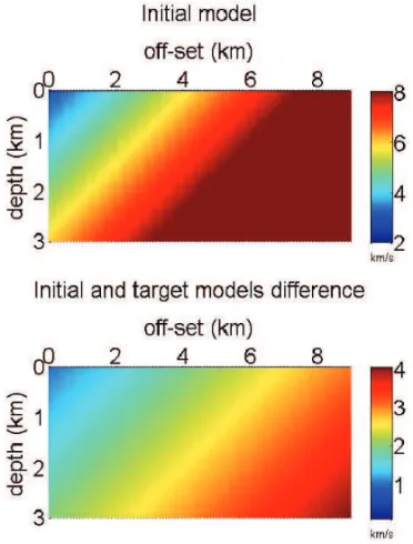
In the case of modelV1, Figure 5 shows the initial model
and its difference in respect of the target model (this difference
is obtained in terms of the least-absolute vector deviation and is approximately 50% when compared to the target model and con-sidering all parameters with the same weight). Employing theL2
vector norm, a difference of 7% is obtained between the inverted and target models. This difference became 5.21% using theL1
integral norm. A graphical view of the inverted models and their differences in respect of the target model can be seen in Figures 6 and 7, utilizing theL2vector norm andL1integral norm,
re-spectively. Results for the considered model can also be seen in Santos & Figueir´o (2007).
Figure 5– In this order: initial model,V1used in both inversion, and difference between initial and target models. This difference is obtained via least-absolute vector deviation and is 50% when compared to the target model with all param-eters being of equal weight.
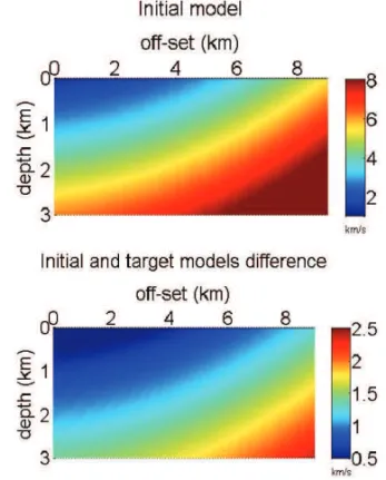
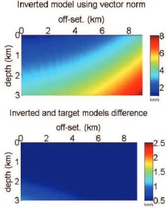
Similarly, an inversion experiment is undertaken involving the model V2. Figure 9 gives graphical views of the initial
model and the difference between initial and target models (cal-culated using least-absolute vector deviation and being approx-imately 30% when compared to the target model and taking into consideration all parameters with the same weight). Using theL2
vector norm, the inverted and target model difference is 19.08% which dropped to 6.47% when theL1integral norm was applied.
Figure 6– Inversion of seismic velocity model,V1utilizing theL2vector norm. In this order: inverted model and difference between inverted and target models. Total processing time: 7 hours (approx.).
Figure 7– Inversion of seismic velocity model,V1usingL1integral norm. In this order: inverted model and difference between inverted and target models. Total processing time: 3 minutes (approx.).
Figure 8– Target seismic compressional wave velocity field model, V2 employed in inversion experiments using both theL2vector norm and L1 integral norm.
Figure 9– In this order: initial modelV2(utilized in both inversions with the two considered norms), and difference between initial and target models. This differ-ence is obtained via least-absolute vector deviation and is 30% when compared to the target model with all parameters being of equal weight.
In addition, the experimental inversion is achieved with the modelV3. Figure 13 gives graphical views of the initial model
and of the difference between initial and target models (this dif-ference is calculated by using the least-absolute vector deviation and is approximately 40% when compared to the target model and taking into consideration all parameters with the same weight). Using theL2vector norm, the inverted and target model
difference is 7.23%, which drops to 6.83% when using theL1
integral norm. A graphical view of the inverted models and their differences in comparison with the target model is shown in Figure 14 (using theL2vector norm) and Figure 15 (using the
Figure 10– Inversion of seismic velocity modelV2using theL2vector norm. In this order: inverted model and difference between inverted and target models. Total processing time: 7 hours and 15 minutes (approx.).
Figure 11– Inversion of seismic velocity field modelV2applying theL1 in-tegral norm. In this order: inverted model and difference between inverted and target models. Total processing time: 5 minutes (approx.).
In this last model, inversions demonstrate high inaccuracy in the estimation of parametersc1,1andc1,2, usingL2vector norm.
The same occurs utilizingL1integral norm withc2,1andc1,2.
For each iteration, the processing time usingL2vector norm is,
approximately, 2 hours, however, with theL1integral norm, this
time was between 12 and 15 seconds. The total time spent in each case, was 9 hours and 50 minutes usingL2vector norm and 5
minutes and 15 seconds usingL1integral norm.
Figure 12– Target seismic compressional wave velocity field model,V3used in inversion experiments employing both theL2vector norm andL1integral norm.
Figure 13– In this order: initial modelV3(used in both inversion: withL2 vec-tor norm andL1integral norm), and difference between initial and target models. This difference is obtained via least-absolute vector deviation and is 40% when compared to the target model with all parameters being of equal weight.
In the case of L1 integral norm, occasionally, during the
singular. Experiments with model V1are carried out using the
same iterative process defined by the Newton method, employing theL1integral norm. The results obtained also presented better
accuracy when compared with a similar experiment using the L2vector norm, with singular matrices not appearing during the
iterative inversion process.
Figure 14– Inversion of seismic velocity modelV3employing theL2vector norm. In this order: inverted model and difference between inverted and target models. Total processing time: 9 hours and 50 minutes (approx.).
DISCUSSIONS
There are scientists who are in agreement that two-point ray tracing is a time-consuming procedure and even dangerous in the vicinity of caustics when using methods like bisection, but disagree about the presence of the stated problems when the method is based on paraxial approximation (Figueir´o & Madariaga, 2000). In respect of these restrictions it could be said that the paraxial method is iterative like bisection, yet, depend-ing on the specific situation, it can be as time-consumdepend-ing as any other method. In addition, the problem with caustics does not dis-appear when we use the paraxial method. For theoretical, experi-mental, specific, or intrinsic use, two-point ray tracing, could possibly be a relatively non time-consuming procedure. How-ever, for tomographic use it is undoubtedly an enormous time consumer. At least 70% of processing time is wasted solving the two-point ray tracing problem, if we assume that we do not want to abuse approximation techniques. It should be stated that in tomography the two-point ray tracing problem must be solved
for each source-receiver pair. It is then solved many times over in all iterations of a tomographic process. In any case, we are not proposing the complete abandoning of ray tracing in tomography as rays are inherent in tomography. We are just proposing a bet-ter use of rays in tomography. In the same way, this work is not a manifesto against ray tracing as we are simply comparing two kinds of norms: this is the essence of the work. If we use an integral norm, ray tracing must be adapted to be conveniently used by such a norm. If we use a more efficient procedure for ray tracing the inversion will be faster.
Figure 15– Inversion of seismic velocity modelV3using theL1integral norm. In this order: inverted model and difference between inverted and target models. Total processing time: 5 minutes and 15 seconds (approx.).
When using integral norm, we benefit from a property of polynomial function, i.e., that polynomials can be easily integ-rated. Figure 3 has a central role, because it expresses the essence of the work and shows the area that we want to minim-ize. However, polynomials are being used to represent data and models, so, in this second case, the oscillatory character of polynomials can cause a few problems during ray tracing, and for this reason we tend to avoid very high-degree polynomials. In addition, as the coefficients of polynomials can vary freely, such parameterization can represent a very large family of models: in fact, an infinite set of models. Oscillations of polynomials can be controlled since we can impose a small value for its derivative. Polynomials can represent realistic though not real oscillations.
For the sake of simplicity, and desire to isolate the experiment from other potential problems, discontinuities in the synthetic observed traveltime data are avoided. However, if the presence of a certain kind of problem is required for a more general experi-ment, calculated data must be considered to also allow discon-tinuities, in order to have appropriate conditions for comparison and adjustment.
CONCLUSIONS
The use of theL1integral norm, instead of theL2vector norm,
in the seismic ray tomography procedures, produces an im-pressive saving in processing time without any significant loss of accuracy (in some cases accuracy actually improves). This saving occurs because when theL1integral norm is used, it is
not necessary to solve the two-point ray tracing problem several times in all iterations of the inversion process. The employed parameterization model is the polynomial, but we believe that this saving of processing time is independent of whatever para-meterization is used. Episodic instabilities occur utilizing the L1integral norm, but this is not especially problematic, as
op-posed to other cases that take place using a different norm. For conceptual reasons and because of strong results, we believe this study will work well when applied to more complicated and real-istic models. In addition, integrals and, more importantly, areas, have a tendency to be more stable (possibly due to their global character) than vectors and points that have just local properties.
ACKNOWLEDGEMENTS
The authors would like to express their gratitude to the State University of Feira de Santana (UEFS) and the Federal Univer-sity of Bahia (UFBA), Bahia, Brazil and to the educational and scientific agency, CAPES (Coordenac¸˜ao de Aperfeic¸oamento de
Pessoal de N´ıvel Superior) for providing the necessary condi-tions for the development of this work.
REFERENCES
BARTLE RG. 1983. Elementos de An´alise Real. Editora Campus Ltda. 429 pp.
BISHOP TN, BUBE KP, CUTLER RT, LANGAN RT, LOVE PL, RESNICK JR, SHUEY RT, SPINDLER DA & WYLD HW. 1985. Tomographic determi-nation of velocity and depth in laterally varying media. Geophysics, 50: 903–923.
BUBE KP & LANGAN RT. 1997. Hybrid L1/L2 minimization with applications to tomography. Geophysics, 62: 1183–1195.
ˇCERVEN´Y V. 1987. Ray Methods for Three-Dimensional Seismic Mod-eling. Lecture notes, Continuing Education Course, University of Trond-heim, NTH and Mobil Exploration Norway Inc., TrondTrond-heim, 830 p.
CLAERBOUT JF & MUIR F. 1973. Robust modeling with erratic data. Geophysics, 38: 826–844.
FIGUEIR ´O WM. 1994. Tomografia de Reflex˜ao no caso de Refletor Curvo. Tese de Doutorado, PPPG-UFBA, Salvador. 150 pp.
FIGUEIR ´O WM & MADARIAGA RI. 2000. A method to avoid arrival caustic points. In: 2000 Technical Program Expanded Abstract, SEG 70thAnnual Meeting, Calgary, Canada. CD-ROM.
GUITTON A & SYMES WW. 2003. Robust inversion of seismic data using the Huber norm. Geophysics, 68: 1310–1319.
LORIS I, NOLET G, DAUBECHIES I & DAHLEN FA. 2007. Tomographic inversion usingL1-norm regularization of wavelet coefficients. Geo-phys. J. Int., 170: 359–370.
LORIS I, DOUMA H, NOLET G, DAUBECHIES I & REGONE C. 2010. Nonlinear regularization techniques for seismic tomography. J. Comp. Phys., 229: 890–905.
MENKE W. 1989. Geophysical Data Analysis: Discrete Inverse Theory. Academic Press, New York, USA. 289 pp.
SANTOS VGB. 2009. Invers˜ao S´ısmica Tomogr´afica usando Norma de Integral de Func¸˜ao. Tese de Doutorado, CPGG-UFBA, Salvador. 91 pp.
SANTOS VGB & FIGUEIR ´O WM. 2006. Invers˜ao s´ısmica tomogr´afica usando trac¸ado anal´ıtico de raios. In: II Simp´osio Brasileiro de Geo-f´ısica, Natal, CD-ROM.
SANTOS VGB & FIGUEIR ´O WM. 2007. Seismic ray reflection tomogra-phy using integral function norm. In: 2007 Technical Program Expanded Abstract, SEG 77thAnnual Meeting, San Antonio, Texas, USA. CD-ROM.
NOTES ABOUT THE AUTHORS
Vˆania Gonc¸alves de Brito dos Santos.Graduated (1992) in Mathematics from Catholic University of Salvador. She received an M.Sc. (1999) in Mathematics (differential geometry) and a Ph.D. (2009) in geophysics (seismic tomography) both from Federal University of Bahia. She is Mathematics Professor at the State University of Feira de Santana since 2001. Her research interests are geophysics and geometry.