Modelling the effects of gravity waves on stratocumulus clouds observed during VOCALS-UK

(1)

ACPD

13, 1717–1765, 2013

Gravity waves and stratocumulus

P. J. Connolly et al.

Title Page

Abstract Introduction

Conclusions References

Tables Figures

◭ ◮

Back Close

Full Screen / Esc

Printer-friendly Version Interactive Discussion

Discussion

P

a

per

|

Dis

cussion

P

a

per

|

Discussion

P

a

per

|

Discussio

n

P

a

per

|

Atmos. Chem. Phys. Discuss., 13, 1717–1765, 2013 www.atmos-chem-phys-discuss.net/13/1717/2013/ doi:10.5194/acpd-13-1717-2013

Atmospheric Chemistry and Physics Discussions

This discussion paper is/has been under review for the journal Atmospheric Chemistry and Physics (ACP). Please refer to the corresponding final paper in ACP if available.

Modelling the e

_ff

ects of gravity waves on

stratocumulus clouds observed during

VOCALS-UK

P. J. Connolly1, G. Vaughan1, P. Cook2, G. Allen1, H. Coe1, T. W. Choularton1,

C. Dearden1, and A. Hill3

1

School of Earth, Atmospheric and Environmental Sciences, The University of Manchester, UK

2

University of East Anglia, UK

3

Met. Office, UK

Received: 18 December 2012 – Accepted: 2 January 2013 – Published: 15 January 2013

Correspondence to: P. J. Connolly ([email protected])

(2)

ACPD

13, 1717–1765, 2013

Title Page

Tables Figures

◭ ◮

Back Close

Full Screen / Esc

Discussion

P

a

per

|

Dis

cussion

P

a

per

|

Discussion

P

a

per

|

Discussio

n

P

a

per

|

Abstract

During the VOCALS campaign spaceborne satellite observations showed that travel-ling gravity wave packets, generated by geostrophic adjustment, resulted in perturba-tions to marine boundary layer clouds over the south east Pacific ocean. Often, these perturbations were reversible in that passage of the wave resulted in the clouds becom-5

ing brighter (in the wave crest) then darker (in the wave trough) and subsequently re-covering their properties after the passage of the wave. However, occasionally the wave packets triggered irreversible changes to the clouds, which transformed from closed mesoscale cellular convection to open form. In this paper we use large eddy simulation (LES) to examine the physical mechanisms that cause this transition. Specifically, we 10

examine whether the clearing of the cloud is due to: (i) the wave causing additional cloud-top entrainment of warm, dry air or (ii) whether the additional condensation of liquid water onto the existing drops and the subsequent formation of drizzle are the important mechanisms. We find that although the wave does cause additional drizzle formation, this is not the reason for the persistent clearing of the cloud; rather it is the 15

additional entrainment of warm, dry air into the cloud, although this only has a signifi-cant e_ffect when the cloud is starting to de-couple from the boundary layer. The result in this case is a change from a stratocumulus to a more cumulus-like regime. For the simulations presented here, cloud condensation nuclei scavenging did not play an im-portant role in the clearing of the cloud. The results have implications for understanding 20

transitions between the different cellular regimes in marine boundary layer clouds.

1 Introduction

It is well recognised that Marine Boundary Layer (MBL) stratocumulus (Sc) clouds are important to climate, due to their large areal coverage and radiative properties (e.g. Bretherton et al., 2004). It is also known that MBL Sc are influenced indirectly by 25

(3)

ACPD

13, 1717–1765, 2013

Title Page

Tables Figures

◭ ◮

Back Close

Full Screen / Esc

Discussion

P

a

per

|

Dis

cussion

P

a

per

|

Discussion

P

a

per

|

Discussio

n

P

a

per

|

Perhaps less discussed in the literature are the connections between synoptic-scale circulations and the properties of MBL Sc.

Recently however, Allen et al. (2012) have presented observations from the Geo-stationary Operational Environmental Satellite (GOES10) during the (VOCALS) field 5

campaign that showed the effects that propagating gravity waves have on the forma-tion of open cellular structures within MBL Sc. In their study, gravity waves propagating horizontally perpendicular to the mean wind were found to modulate the height of the cloud-topped boundary layer over the South East Pacific (SEP) by up to 400 m peak-to-trough. They were found to induce both reversible and irreversible changes in the 10

cloud-radiative and dynamical properties, such that a region of clear sky was evident in the trough of the passing wave fronts, which in some cases persisted and devel-oped into so-called pockets of open cells. Allen et al. showed that the epicentre of the waves coincided with a large negative residual in non-linear balance close to the po-sition of the subtropical jet stream. This therefore suggested that the source of energy 15

for the waves was geostrophic adjustment in the sharply divergent flow associated with a disturbed jet stream.

The mechanism for the clearing of the cloud was briefly discussed by Allen et al. al-though not addressed fully and left for further work. The presence of increased rain in the crest of the waves, observed using the Advanced Microwave Sounding Radiometer-20

EOS (AMSRE) and the Moderate Resolution Imaging Spectroradiometer (MODIS) pro-vided evidence that the mechanism might be due to the cloud layer being “rained out” because of increased condensation of water vapour onto the cloud drops, followed by their collision and coalescence to form rain drops, which then fell out of the cloud. They noted that this is a likely mechanism because the cloud appeared to transition to clear 25

sky in limited regions only, which were thought to be regions of higher liquid water path (LWP) or lower drop number concentration.

(4)

ACPD

13, 1717–1765, 2013

Title Page

Tables Figures

◭ ◮

Back Close

Full Screen / Esc

Discussion

P

a

per

|

Dis

cussion

P

a

per

|

Discussion

P

a

per

|

Discussio

n

P

a

per

|

and closed cells are two of the most frequent types of cloud self-organisation, ob-served within Sc, referred to as mesoscale cellular convection (MCC) (Hubert, 1966). The “open” and “closed” descriptors apply if the central part of the cell is clear or cloudy respectively; however, less frequent forms of self-organisation are also formed within 5

Sc, such as actinoform clouds (see overview by Garay et al., 2004). Furthermore, both open and closed forms of MCC bear a striking resemblance to Rayleigh-B ´enard con-vection (Agee, 1984), which is well studied. Although the mechanisms responsible for the transition from closed to open cell forms are unclear, it is evident that the two cellu-lar regimes form when the boundary layer is deeper than∼1 km and that closed cells 10

form over cold ocean currents, while open cells form preferentially over warm ocean currents (see Wood and Hartmann, 2006, and references therein).

Wood et al. (2011a) presented an aircraft study of the transition from closed to open cellular convection observed during the VOCALS campaign. They found that the POCs consisted of intermittent precipitating (Cu) clouds that detrained into very optically thin 15

stratiform cloud. A key finding was that the precipitation rates within the POCs were not significantly different to those within the closed cell regime, leading to the argument that precipitation is not a sufficient condition for the formation of POCs. This is a significant finding and one that is highly relevant to this study. However, it was clear from the Wood et al. work that the cells within the POCs were often surrounded by a “boundary cell” 20

with divergent cold pools at lower levels, convergence in the middle of the boundary layer and divergence at the top, thus suggesting that precipitation processes may play a role in maintaining the POCs once they form. Further evidence of the importance of precipitation processes was that the deeper clouds within the POCs detrained air that was very low in CCN concentrations, thus CCN scavenging by drizzle was thought to 25

be very efficient.

(5)

ACPD

13, 1717–1765, 2013

Title Page

Tables Figures

◭ ◮

Back Close

Full Screen / Esc

Discussion

P

a

per

|

Dis

cussion

P

a

per

|

Discussion

P

a

per

|

Discussio

n

P

a

per

|

waves and can often generate spurious gravity waves due to the numerical methods employed. Indeed the Unified Model (UM) used in the Knippertz et al. study was unable to accurately capture the wavelength of a pre-frontal gravity wave when run at 4 km 5

resolution.

In this study we take the findings of Allen et al. (2012) further by performing semi-idealised LES modelling of MBL Sc upon which we impose the effects of gravity waves. Due to the relatively small domain sizes employed and the difficulties in capturing the dynamics of gravity waves within numerical models, we do not focus on the details of 10

wave generation. Rather, we look at the sensitivity of the Sc to lifting and lowering of the layer by a “kinematic gravity wave”, the details of which are specified from observed GOES10 imagery, to examine the physics behind the clearing of the Sc. We point out that the gravity wave packets under consideration in this paper have a different source to the ‘upsidence’ wave described by Rahn and Garreaud (2010), which is due 15

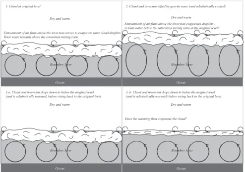
to mechanical blocking by the Andes of the westerly flow above the boundary layer. There are two hypotheses to be tested. These are that the clearing and consequent breaking up of the cloud is a result of:

1. increased entrainment of dry air into the cloud layer, which reduces the total water content to levels below the saturation vapour mixing ratio at the initial altitude of 20

the cloud level. This results in evaporation of the cloud when it descends to the original level.

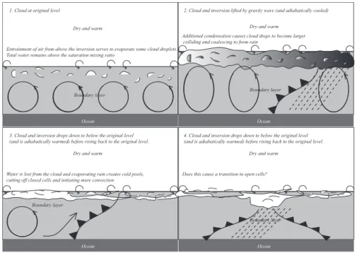
2. additional condensation followed by collision and coalescence, which leads to drizzle falling out of the cloud. This drizzle then evaporates below the cloud, cool-ing the air below and cuttcool-ing o_ffthe boundary layer thermal and moisture circula-25

tion.

(6)

ACPD

13, 1717–1765, 2013

Title Page

Tables Figures

◭ ◮

Back Close

Full Screen / Esc

Discussion

P

a

per

|

Dis

cussion

P

a

per

|

Discussion

P

a

per

|

Discussio

n

P

a

per

|

turbulence and mixing at cloud top. Both mechanisms appear to be plausible, but it is important to understand which is the dominant mechanism so that if parameterisations are to be developed they may take account of the relevant physics and thus be more 5

realistic.

2 Background to the VOCALS study

The VOCALS project took place from 15 October to 15 November 2008 in the SEP to investigate the interactions between land, sea and atmosphere with the aim of im-proving representation of processes in the region in both global and regional models. 10

Detailed descriptions of the international effort have been presented and discussed in the scientific literature (e.g. Wood et al., 2011b; Allen et al., 2011; Wood et al., 2011a) and so the details will not be repeated here, rather we will present an overview of the campaign and discuss the measurements relevant to this paper.

The observations of gravity wave packets affecting MBL Sc were taken from GOES10 15

on several days, although the clearest evidence was on the 8th October 2008. Unfor-tunately there were no in-situ observations on this day and so the model simulations presented in this paper are idealised and have been developed from observed statistics taken from VOCALS flight data (Bretherton et al., 2010; Allen et al., 2011).

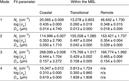
Allen et al. (2011) partitioned the VOCALS measurement into 3 regions, based on 20

the location from the shore. These were: Coastal (to the east of 75◦W); Transitional (between 75◦W and 80◦W) and Remote (to the west of 80◦W). They presented quad-lognormal fits to the median of the number-size distributions of aerosol particles mea-sured in the MBL for each of these regions (these are shown in Table 2). The data show a clear trend of decreasing accumulation mode aerosol concentrations moving 25

(7)

ACPD

13, 1717–1765, 2013

Title Page

Tables Figures

◭ ◮

Back Close

Full Screen / Esc

Discussion

P

a

per

|

Dis

cussion

P

a

per

|

Discussion

P

a

per

|

Discussio

n

P

a

per

|

likely play a role in determining the location of POCs over the region, which tend to occur most frequently in the transition region and perhaps the remote region.

Figure 3 shows a case study that Allen et al. (2012) presented of a gravity wave 5

triggering the formation of POCs within an area of otherwise overcast Sc. Throughout the day several gravity wave packets propagated in a north-east direction and eventu-ally resulted in the cloud opening up (Fig. 3, centre) at 79 to 81◦W. This persisted and became more prevalent throughout the day (Fig. 3, right). The study will now focus on determining the mechanism that causes the cloud to clear.

10

3 Methodology

3.1 Large eddy modelling

Version 2.4 of the UK Met.Office (Met.Office) large eddy model (LEM) (Gray et al., 2001) was used to simulate the interaction between dynamics, microphysics and radi-ation for an idealised case based on observradi-ations from the VOCALS campaign. 15

The LEM is an anelastic, nonhydrostatic numerical model, with prognostic equa-tions for the advection of momentum, mass continuity and the advection and diffusion of scalars such as potential temperature and moisture variables. The LEM explicitly resolves large scale turbulent motions, which are responsible for most of the turbulent energy and transport, while parametrising sub-grid motions with a first order turbulence 20

scheme.

All of the simulations presented use a vertical domain extending from the surface to 3 km while the horizontal domain is 16×16 km in extent. The horizontal resolution (∆x,

∆y) is 120 m and the vertical resolution (∆z) 20 m below the inversion. Starting 100 m above the inversion to an altitude of 2000 m the vertical grid spacing was stretched to 25

(8)

ACPD

13, 1717–1765, 2013

Title Page

Tables Figures

◭ ◮

Back Close

Full Screen / Esc

Discussion

P

a

per

|

Dis

cussion

P

a

per

|

Discussion

P

a

per

|

Discussio

n

P

a

per

|

The simulation time for all cases is 12 h with a variable time step to satisfy two sepa-rate Courant-Friedrichs-Lewy (CFL) criteria. The first criterion was that the Courant number, ∼u×∆t

∆x≤0.2, and the second was that the viscous stability parameter,

5

∼4∆tν

∆x2 ≤0.2, whereνis the viscosity of the flow, the dependence of which has a pa-rameterised relation to the resolved part of the flow. The maximum time-step is limited to 5 s .

In all simulations the roughness length is set to 2.0×10−3m for momentum and 2.0×10−4m for scalars, consistent with values for an open sea surface. A sponge 10

layer is applied to the top 500 m of the domain, so that fields are relaxed back to initial conditions in this region. All simulations employ cyclic lateral boundary conditions.

To initialise the model the vertical profiles of horizontal wind were set to a con-stant u=7.0 m s−1 and v=−1.0 m s−1. The initial cloud liquid water content was set to be adiabatic leading up to the inversion and specified to be horizontally homoge-15

neous throughout the model, while the initial drop number concentration was set to be 100 mg−1of air. The total number of CCN was set to be 500 mg−1 of air below the inversion and to zero above the inversion, which is consistent with the VOCALS re-gion (Allen et al., 2011) for the purpose of a relative contrast between the MBL and free-troposphere; however, there were episodes where pollution was transported large 20

distances resulting in discrete layers of higher CCN concentrations that may have been entrained into the MBL (this effect is not addressed in the current study).

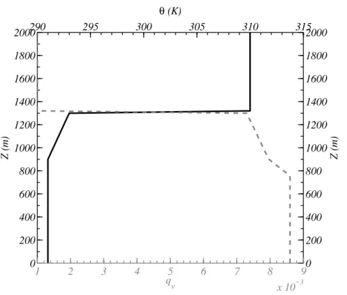
The potential temperature, θ, and vapour mixing ratio, qv, were initialised with an

idealised sounding that sets θ=291 K from the ground to an altitude of 900 m and

θ=310 K above the inversion height of 1350 m, withθ=293 K just below the inversion. 25

From 900 m to just below the inversion the potential temperature increased linearly. Vapour mixing ratio,qv, was set to 8.6×10

−3

(9)

ACPD

13, 1717–1765, 2013

Title Page

Tables Figures

◭ ◮

Back Close

Full Screen / Esc

Discussion

P

a

per

|

Dis

cussion

P

a

per

|

Discussion

P

a

per

|

Discussio

n

P

a

per

|

To promote turbulence a random perturbation with maximum magnitude of ±0.1 K was applied to the initial potential temperature field below the inversion; no perturbation was added above the inversion. Both the wind and the geostrophic wind were set to 7 m s−1 in the x direction and −1 m s−1 in the y direction. Geostrophic wind forcing 5

is required to maintain the horizontal winds, otherwise the e_ffects of surface friction would reduce the wind speed throughout the simulation. The model was also run with interactive shortwave and longwave radiation (Edwards and Slingo, 1996), which was updated every 150 s, model time. Rather than use a set droplet e_ffective radius for the radiative transfer scheme it was diagnosed from the microphysics scheme, which 10

allows the so called Twomey effect to be accurately modelled. Large scale divergence was specified to be 3×10−6s−1, which is consistent with both QuikSCAT and Weather Research and ForecastModel (WRF) simulations for the period in question (Rahn and Garreaud, 2010) and helps to maintain the inversion.

The microphysics scheme used was a 2-moment scheme for both cloud water and 15

rain water fields and based on that by Morrison et al. (2005), but with prognostic CCN. In accord with the in-situ observations, the representation of the raindrop size dis-tribution within the LEM microphysics scheme was parameterised as an exponential distribution.

The rate of warm rain formation was parameterised using the auto-conversion 20

scheme described by Seifert and Beheng (2005). This scheme requires that the cloud drop size distribution is input as a modified gamma distribution in mass:

d N dx =Arx

ν

rexp (−Bx) (1)

wherex is the drop mass. Short comings of assuming such a distribution are acknowl-edged, since larger drizzle drops tend to sediment out of the cloud (Dearden et al., 25

(10)

ACPD

13, 1717–1765, 2013

Title Page

Tables Figures

◭ ◮

Back Close

Full Screen / Esc

Discussion

P

a

per

|

Dis

cussion

P

a

per

|

Discussion

P

a

per

|

Discussio

n

P

a

per

|

this reason, following Morrison et al. (2005), we use a parameterisation for effective ra-dius in stratocumulus clouds (Martin et al., 1994). Accurate derivation ofνr, rather than

specification of a constant, is an important step since the rate of warm rain formation 5

(Eq. 1) is quite sensitive to this parameter in the Seifert and Beheng (2005) scheme. The microphysics scheme also has a field for prognostic CCN, which interacts with the cloud fields, therefore having consistent sources and sinks. Observational data were used to constrain the CCN within the model as described in Section 3.1.2.

3.1.1 Gravity wave kinematics

10

The gravity wave properties were derived from GOES10 satellite observations of ness temperature in the thermal infrared. The approximation was made that the bright-ness temperature was equal to the temperature of the top of the cloud and that the initial lifting (before precipitation occurred) was adiabatic. This allowed us to quantify the wavelength and amplitude of the gravity wave packet.

15

The observations showed that the wave was monochromatic (Allen et al., 2012), and non-dispersive. Hence, the phase velocity,vp=ωk, could be calculated using

consecu-tive images to see how far the wave crests travelled in a time-period.

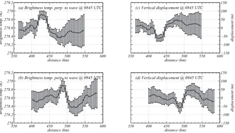
In order to do this we took two consecutive GOES10 satellite images, taken an hour apart, and drew a rectangular box perpendicular to the wave front. We then calculated 20

means and standard deviations of the brightness temperatures as a function of dis-tance perpendicular to the wave front. Figure 5 show two GOES10 images that depict this procedure, with the rectangles showing the area over which statistics were taken.

The statistics of the wave derived from the two images in Fig. 5 are shown in Fig. 6a and b. A clear wave structure is seen in the fields of brightness temperature, with 25

(11)

ACPD

13, 1717–1765, 2013

Title Page

Tables Figures

◭ ◮

Back Close

Full Screen / Esc

Discussion

P

a

per

|

Dis

cussion

P

a

per

|

Discussion

P

a

per

|

Discussio

n

P

a

per

|

be seen that the wave has moved around 55 km in distance from its original location at 08:45, hence the phase velocity of the wave,v_p∼55×10

3

3600 ∼15.3 m s

−1

.

In order to convert the difference in brightness temperature to a displacement in al-titude we assume that the wave lifting is adiabatic. At∼280 K the saturated adiabatic 5

lapse rate is approximately 6 K km−1 and so this can be used to convert the bright-ness temperatures to a displacement. Figures 6c and d suggest that the amplitude of the wave was around 50 to 100 m, at least for the period shown. In other case (not discussed here) the amplitude of the wave could extend to around 150 to 250 m.

Due to computational constraints our model domain was only 16×16 km in the hor-10

izontal. Figure 7 superimposes such a domain on a satellite image, showing it to be considerably smaller than the scale of convective organisation; thus we cannot aim to represent an MCC. Further, the domain is much smaller than the gravity wave wave-length (∼100 km), so we cannot model the passage of the wave across the domain either. Rather, we restrict this study to an investigation of the physics leading to cloud 15

clearing, by applying a wave perturbation uniformly across the domain. This perturba-tion is generated by modulating the subsidence velocity in the model.

The properties of a time-dependent stationary wave that this produces can be de-rived from the properties of the travelling wave through the relation between phase velocity,v_p, wave number,k=2_λπ, and angular velocity,ω=2_Tπ, i.e.:

20

v_p=ω k =

λ

T (2)

therefore, we can derive the period of the equivalent stationary wave to beT =vλp ∼

100×103

15.3 ∼6500 s.

(12)

ACPD

13, 1717–1765, 2013

Title Page

Tables Figures

◭ ◮

Back Close

Full Screen / Esc

Discussion

P

a

per

|

Dis

cussion

P

a

per

|

Discussion

P

a

per

|

Discussio

n

P

a

per

|

surface (to satisfy the gravity wave boundary condition). Thus we linearly increased the amplitude of the wave from zero at the surface toAat the height of the inversion:

z(z,t)=

      

z+Az_z_i sin2π[t−t0] T

ifz≤z_i

z+Asin2π[t−t0] T

ifz > zi zift < t0ort > t0+n×T

(3)

wherezis the altitude,tis time,z_i is the height of the inversion,t0is the time when the

wave starts,T is the period of the wave,nis the number of cycles of the wave that the 10

cloud is subject to, andAis the wave amplitude. Differentiating Eq. (3) wrt time yields the velocity:

w(z,t)₌

      

Az

z_i ×2Tπcos

₂_π_[_t₋_t

0]

T

ifz≤z_i

A×2_Tπcos

₂_π_[_t₋_t

0]

T

ifz > zi

0 ift < t0ort > t0+n×T

(4)

wherewis the vertical wind to be added to the subsidence forcing in the model. The gravity wave therefore does not directly affect the small scale dynamics within 15

the Sc deck, but does so indirectly, through the inhomogeneities brought about by extra condensation and warm rain formation.

A key question is thus: what are the threshold wave amplitudes or number of waves required to produce an irreversible change in the Sc cloud?

3.1.2 CCN activation and parcel modelling

(13)

ACPD

13, 1717–1765, 2013

Title Page

Tables Figures

◭ ◮

Back Close

Full Screen / Esc

Discussion

P

a

per

|

Dis

cussion

P

a

per

|

Discussion

P

a

per

|

Discussio

n

P

a

per

|

CCN activated depends on the peak updraft velocity at cloud base. In fact we used the more common approximation found in Rogers and Yau (1989):

NCCN=0.88×C2/(2+k)×

70×w3/2

(k/(2+k))

(5)

whereNCCN is the drop concentration (cm

−3

) at cloud-base, w the updraught speed in m s−1andC(cm−3) andkare constants describing the supersaturation activity of the 10

CCN—NCCN=Cs

k

, wheres is the supersaturation in percent. This approach requires the constants C and k, which were derived by applying a parcel model (described below) to aerosol data taken from the BAe-146 Facility for Airborne Atmospheric Mea-surements (FAAM) aircraft meaMea-surements presented in Allen et al. (2011).

Aerosol size distributions in the MBL over the SEP were measured on board the 15

BAe-146 FAAM aircraft using an Scanning Mobility Particle Sizer (SMPS) and a Pas-sive Cavity Aerosol Spectrometer Probe (PCASP) as described by Allen et al. (2011). The chemical composition of the aerosol was measured with a Droplet Measurement Technologies (DMT) Aerosol Mass Spectrometer (AMS) and found to be predominantly sulphate internally mixed with a small amount of organics.

20

In order to observationally constrain CCN in the LEM, quad-lognormal fits to the SMPS and PCASP data (see Allen et al., 2011, which are repro-duced in Table 2) were used as input to the Aerosol-Cloud-Precipitation In-teraction Model (ACPIM), bin-microphysics, parcel model (see Connolly et al., 2009, 2012) and the model was run for ten different updraft speeds: w= 25

(14)

ACPD

13, 1717–1765, 2013

Title Page

Tables Figures

◭ ◮

Back Close

Full Screen / Esc

Discussion

P

a

per

|

Dis

cussion

P

a

per

|

Discussion

P

a

per

|

Discussio

n

P

a

per

|

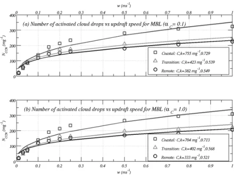
modelling were pressure,P =950 mbar; temperature,T =11◦C and relative humidity, RH=0.95. The model was run for a total ascent of 200 m, at which point the number of activated cloud drops was determined.

The results of the ACPIM parcel modelling are shown in Fig. 8a and b, which shows only a small sensitivity toα_C in the range 0.1≤α_C ≤1.0. As expected, the number of 10

CCN decreases with increasing distance from the coast, although there is little drop o_ff in CCN concentrations when moving from the transition region to the remote re-gion. In the context of this study the coastal CCN concentrations will be referred to as “high”; transitional will be referred to as “medium”; and remote will be referred to as “low”. It is recognised that these CCN values do not represent a large variation in 15

CCN number concentration, nevertheless the descriptors, “high”, “medium” and “low” are relevant in the context of this study. All runs, unless explicitly stated, used ‘medium’ CCN concentrations.

3.2 Sensitivity studies with the LEM

The LEM was used to investigate the effect of the imposed wave on the dynamics 20

and microphysics of the stratocumulus clouds. A number of model runs based on the methodology described in Sects. 3.1,3.1.1 and 3.1.2 were performed which, for com-pleteness, are listed in Table 1.

4 Results-LEM simulations

Here we present results from the LEM simulations to show the sensitivity to the forcing imposed by gravity waves. The results are organised into four main sections, dealing with the effects of the amplitude of the gravity waves on the response of the modelled MBL Sc; the e_ffect of including multiple waves of amplitude, A=150 m; the e_ffect of wave timing, specifically waves occurring at night and during daytime; and the effects 5

(15)

ACPD

13, 1717–1765, 2013

Title Page

Tables Figures

◭ ◮

Back Close

Full Screen / Esc

Discussion

P

a

per

|

Dis

cussion

P

a

per

|

Discussion

P

a

per

|

Discussio

n

P

a

per

|

Firstly, we present images of the modelled LWP for two of the simulations: one with-out any imposed gravity wave forcing and one with a single 150 m amplitude gravity wave initiated at 05:00 local time. Figure 9 shows the results of these two simulations and shows that the effect of the wave is to firstly increase the LWP (Fig. 9a and e) fol-10

lowing which the cloud clears and breaks up in the downward part of the wave (Fig. 9b and f). However, the LWP soon recovers almost to previous values (Fig. 9c and g), but then starts to break up towards the end of the simulation (Fig. 9d and h). Although there are similarities to the satellite images presented in Fig. 3, it is apparent that the modelled clouds take much longer to clear (some 8 h after the occurrence of the wave), 15

whereas in the observations clearance occurred almost immediately after the passage of the wave. The model results in this case are not therefore consistent with the obser-vations.

4.1 E_ffect of wave amplitude

As there was some variability in the amplitude of the observed gravity waves we have 20

looked at the e_ffect of wave amplitude on the MBL Sc. Figure 10 shows the results of this set of simulations. It is seen that the case without any gravity waves results in almost completely overcast conditions, whereas the cases with waves all result in a slow clearing of the cloud, some 8 h after the occurrence of the wave. While there are some subtleties it is apparent that in these simulations wave amplitude does not have an appreciable effect on the clearing of the cloud. However, it is noteworthy that the 300 m wave results in the MBL Sc taking longer to fill in after the occurrence of the wave at∼06:50 local time. It may therefore be that waves with higher amplitudes than 300 m would result in a rapid clearing of the cloud; however, such high amplitudes were 5

(16)

ACPD

13, 1717–1765, 2013

Title Page

Tables Figures

◭ ◮

Back Close

Full Screen / Esc

Discussion

P

a

per

|

Dis

cussion

P

a

per

|

Discussion

P

a

per

|

Discussio

n

P

a

per

|

4.2 Effect of multiple waves

It is clear from the GOES10 imagery that a gravity wave train can contain multiple peaks and troughs. Hence we decided to examine the sensitivity of the modelled MBL Sc to the number of gravity wave oscillations, by including 1, 2, 3 or 4 successive cycles 10

of the wave. Fig. 11 shows a comparison of modelled LWP, comparing a case with no gravity waves to a case with four successive gravity waves. In this figure e, f and g show times in the downward moving part of the wave and hence show the cloud breaking up after an initial increase in LWP prior to this. When comparing these to the equivalent times without a gravity wave (a, b and c) it can be seen that each time a wave occurs 15

it results in an increase in the amount of broken cloud. Figures 11d and h show the cloud at the end of the model simulations, long after the waves occurred, where it is clear that the case with four waves has resulted in a significant amount of clearing of the cloud layer.

To look at the effect of multiple numbers of wave in more detail we present the cloud 20

cover percentage time-series in Fig. 12. In this Figure it can be seen that the simula-tion with two waves results in a slight clearing of the cloud layer at about 08:10 local time, which takes a while to fill back in, before clearing again in a similar way to the single wave cases in Fig. 10. However, the simulations with both 3 and 4 waves are significantly different. The case with 3 waves results in a sudden change in the total 25

cloud coverage to about 60 %, which then decreases to almost zero at the end of the simulation, whereas the case with 4 waves results in an even more dramatic change in the total cloud cover; however, cloud coverage then increases slowly as the simulation progresses. In fact, this increase in cloud coverage is associated with more intense turbulence and more Cu-like clouds, which is suggestive of a change in convective 5

(17)

ACPD

13, 1717–1765, 2013

Title Page

Tables Figures

◭ ◮

Back Close

Full Screen / Esc

Discussion

P

a

per

|

Dis

cussion

P

a

per

|

Discussion

P

a

per

|

Discussio

n

P

a

per

|

4.3 Effect of timing of the wave

To attempt to answer the question of whether the cumulative effect of multiple waves was important or whether it is the timing that is important we ran two simulations using single 150 m waves, but altered the time of day at which they occurred: (i) the time at 10

which the 3rd wave occurred in the 3 and 4 wave simulations “single-3rd wave” and (ii) the time at which the 4th wave occurred in the 4 wave simulation “single 4th wave”. The LWP fields from these simulations are shown in Fig. 13. Figs. 13a and e show the LWP before any gravity wave perturbations have been applied, whereas Fig. 13b shows a time just after the wave in the “single 3rd wave” simulation with Fig. 13f being the same 15

time for the “single 4th wave” simulation. Figure 13g shows the time just after the wave in the “single 4th wave” simulation. By this time both simulations display broken cloud, the level of which increases towards the end of the simulation (Fig. 13d and h). So here it is apparent that the timing of the wave is crucial to its effect on the MBL Sc.

The results of the simulations shown in Fig. 13 are compared to the “no wave” case 20

and summarised in terms of total cloud cover in Fig. 14. Here it is apparent that the “single 3rd wave” simulation does not result in a dramatic reduction in total cloud cover, but it does take time to fill back in to 100 %, before breaking up again in a similar way to all single wave cases. However the “single 4th wave” case does result in a clear reduction in cloud coverage, although not quite as dramatic as the case that included 25

4 cycles of the wave. There is no strong evidence for a change in convective regime, like in Fig. 12. It is therefore apparent that both the timing and the number of waves affect cloud clearing. A point worth noting is that there was more drizzle in the case with multiple waves and this had an impact on the development of weak cold pools in the MBL, which increased convective instability.

Fig. 14 and 15a suggests that at 9:00 the boundary layer is still strongly coupled to the surface fluxes of moisture; this is why the “single 3rd wave” case does not result in a clearing of the cloud layer. However, by approximately 11:00 (or just after) it appears 5

(18)

ACPD

13, 1717–1765, 2013

Title Page

Tables Figures

◭ ◮

Back Close

Full Screen / Esc

Discussion

P

a

per

|

Dis

cussion

P

a

per

|

Discussion

P

a

per

|

Discussio

n

P

a

per

|

of the cloud layer from the lower level fluxes may be demonstrated by a vertical profile of the variance of vertical velocity,w′_w′_.

Figure 15a,b show the variance of the vertical velocity for 5 model simulations: the ‘no wave’ case; the ‘single 1st wave’ case; the case with 4 150 m waves and the “single 10

3rd wave” and “single 4th wave” case. Figure 15a shows the variance of vertical velocity at 09:00 showing thatw′_w′ _{is reasonably high in the cloud region for all cases except}

the simulation with 4 wave cycles. It should be noted that at 09:00 in both the simulation with 4 wave cycles and the “single 3rd wave” case wave subsidence is occurring, which effectively lowers the inversion by 150 m.

15

Figure 15b shows the corresponding variance of vertical velocity at 12:00 and shows a significant reduction in the velocity variance for all simulations, with a weight-ing towards higher variances near the surface, thus signallweight-ing the decouplweight-ing of the cloud from the surface fluxes. It is noticeable that both the simulation with 4 waves and the “single 4th wave” case have lower variance of vertical velocity in the region 20

600< Z <1200 m than the other cases at this time. Although not shown here, analysis of the variance of vertical velocity at the end of the simulations shows that, of all of the simulations, the case with 4 waves leads to the highest variances throughout the depth of the boundary layer. Although this demonstrates some degree of coupling, it is not homogeneous across the model domain and is more similar to Cu type convection. 25

4.4 Evolution of cloud throughout the day

Figure 16 shows the evolution of cloud-top and cloud-base altitude from a simulation with no wave and three simulations with a 150 m that occurred at the time of the 1st; 3rd and 4th wave in the 4 wave simulation. These are referred to as the “single 1st wave”; “single 3rd wave” and “single 4th wave” simulations respectively. It can be seen that the thickness of the cloud layer, in all simulations, is reduced throughout the day, due to absorption of solar radiation and the resultant warming of the boundary layer, 5

(19)

ACPD

13, 1717–1765, 2013

Title Page

Tables Figures

◭ ◮

Back Close

Full Screen / Esc

Discussion

P

a

per

|

Dis

cussion

P

a

per

|

Discussion

P

a

per

|

Discussio

n

P

a

per

|

It is shown that cloud-top altitude after the “single 3rd wave” and “single 4th wave” simulations is lower than the “no wave” case. This is similar for the cloud-base altitude. In both cases the difference is considerably greater than in the “single 1st wave” case. The lowering of the cloud-top is an indicator of cloud-top entrainment; hence, these 10

results suggest that there is not much enhancement of cloud-top entrainment in the ‘single 1st wave’ case. This is a qualitative demonstration that entrainment is enhanced in the cases with imposed gravity-waves and that the timing of the wave is crucial to the e_ffect that cloud-top entrainment has on the evolution of the cloud.

4.5 Effect of warm rain formation

15

The importance of multiple successive waves may suggest that each time the cloud layer is lifted the resulting warm rain acts to reduce the LWP resulting in a cumulative e_ffect on the clearing of the cloud. Warm rain generation was indeed seen in the model fields each time the cloud layer was lifted; however, this rarely reached the surface in the model, as it evaporated during its descent. In order to ascertain the importance of 20

the warm rain process we ran an additional model simulation with the warm rain auto-conversion scheme switched offfor the case with 4 successive waves. The results of this are summarised in Fig. 17. Here it can be seen that both cases result in a clearing of the MBL Sc, therefore suggesting that the main process responsible for clearing the cloud is not the warm rain process itself. However, we note that the simulation with 25

warm rain results in a change in convective regime later in the simulations (as shown by the more rapid increase in total cloud coverage near the end of the simulation). Other analyses of the variance of vertical velocity (not shown) indicate that the “4×150 m wave” case with rain has much higher variances in the cloud layer at the end of the simulations compared to the same case without warm rain. The reason for this is that the evaporation of rain below cloud destabilizes the boundary layer so that the cloud layer has better coupling to the surface fluxes of moisture. Also worthy of note is that 5

(20)

ACPD

13, 1717–1765, 2013

Title Page

Tables Figures

◭ ◮

Back Close

Full Screen / Esc

Discussion

P

a

per

|

Dis

cussion

P

a

per

|

Discussion

P

a

per

|

Discussio

n

P

a

per

|

part of the wave, which is as expected since warm rain removes total water from the cloud layer.

4.6 Influence of CCN concentration

It is interesting to investigate whether CCN concentrations play a role in the clearing 10

of the cloud. POCs were observed to form preferentially in the transition and remote region and CCN concentrations for all three regions are described in Section 3.1.2 and shown in Fig. 8. To investigate the role of CCN two additional simulations were per-formed, both including warm rain processes. One was a 300 m wave with “high” CCN and the other was a 150 m wave with ‘low’ CCN. These were chosen to demonstrate 15

whether: (i) ‘high’ CCN could suppress the slow clearing of the cloud that occurred 8 h after the wave (Fig. 10) and (ii) “low” CCN could lead to additional clearing of the cloud due to warm rain.

Fig. 18(left) shows the time-series of total cloud cover for these simulations. The re-sults show that the 300 m wave with “high” CCN rere-sults in a cloud with almost 100 % 20

cloud coverage. This is in contrast to the simulation with a 300 m wave (and ‘medium’ CCN), which resulted in a clearing of the cloud. The reason for this is that the case with higher CCN resulted in more cloud top radiative cooling (because the cloud droplets were smaller and more numerous), an e_ffect that was able to maintain the cloud cover-age at higher values due to additional condensation.

25

The simulation with a 150 m wave and “low” CCN failed to clear the cloud. More warm rain was produced in this case than the simulation with a 150 m wave and medium CCN, which resulted in lower cloud coverage at 11:00; however, the cloud coverage then recovered, presumably because this moistened and cooled the air below the cloud and resulting in a more coupled boundary layer. Hence, it appears that CCN do play an important role in the clearing of the cloud. The intermediate CCN values away from the coast are more likely to result in a clearing of the cloud than both the higher CCN values close to the coast and the lower CCN values away from the coast. Although the 5

(21)

ACPD

13, 1717–1765, 2013

Title Page

Tables Figures

◭ ◮

Back Close

Full Screen / Esc

Discussion

P

a

per

|

Dis

cussion

P

a

per

|

Discussion

P

a

per

|

Discussio

n

P

a

per

|

the means from the three regions (coastal, transitional and remote) it is encouraging that using observationally constrained CCN within the LEM is able to provide insights into some of the reasons why the clearing of cloud occurs preferentially in the transition region. It is also likely that boundary layer height plays an important role in the clearing 10

of the cloud; however, this e_ffect is not investigated here.

Figure 18(right) shows the time-series of the domain-averaged LWP for the CCN simulations. It can be seen that LWP increases during the crest of the wave, decreases during the trough and then increases to values that are below those seen in the ‘no wave’ case. Also evident is that higher CCN results in higher LWPinitially, but later in 15

the simulations the opposite is true (e.g. compare ‘150 m wave’ with “150 m wave low aerosol” and “300 m wave” with “300 m wave high aerosol”).

4.7 Effect of cloud-top entrainment

In order to probe whether entrainment of dry air from aloft may be responsible for cloud clearance we initialised a passive tracer in the model, set to 1.0 above the inversion 20

and zero below the inversion (Fig. 19a). Figure 19b shows the horizontal mean of the tracer field in the model at 12:00 local time. This shows some mixing of the tracer from above the inversion into the boundary layer for all model runs.

Interestingly the run with one 150 m gravity wave occurring early in the morning has a tracer distribution that is almost the same as the case without any wave; hence the 25

single, early gravity wave does not cause any additional mixing. When 4×150 m waves are used for the forcing there is much more mixing of air above the inversion into the cloud layer. In addition a similar effect happens when we use a single 150 m gravity wave that occurs later in the day (“single 4th wave”). Therefore, the tracer results sug-gest that it is the mixing in to the cloud of warm, dry air from above the inversion that causes the rapid evaporation of the cloud shortly after the wave. The eddies respon-sible for the mixing of dry air into the cloud were resolved in the model wind-field as can be seen in the variance of the vertical velocity (Fig. 15), and were a result of latent 5

(22)

ACPD

13, 1717–1765, 2013

Title Page

Tables Figures

◭ ◮

Back Close

Full Screen / Esc

Discussion

P

a

per

|

Dis

cussion

P

a

per

|

Discussion

P

a

per

|

Discussio

n

P

a

per

|

5 Discussion

The model results suggest that gravity waves are able to result in a rapid clearing of the cloud only after sunrise. In the simulations presented this is likely related to the fact that the Sc starts to become de-coupled after sunrise. De-coupling of the boundary layer 10

was a common occurrence away from the coastal region during the VOCALS campaign (Jones et al., 2011), even in the mid-morning, before solar insolation leads to stronger decoupling; however, despite the decoupling there was often 100 % cloud cover. In our simulations, when there is strong coupling between the sea and the cloud-topped boundary layer, gravity waves do not cause a rapid clearing of the cloud as the fluxes 15

of water vapour from the ocean surface are able to fill in the cloud rapidly. However, when gravity waves occur in Sc that are coupled (for instance before sunrise in the simulations) they do result in aslow clearing towards the end of the simulations.

Weak coupling between the surface and cloud means that moist air does not contin-uously cycle through the boundary layer; hence, the entrainment of dry air from aloft, 20

which follows the gravity wave, serves to evaporate the cloud. Once most of the cloud has evaporated due to the warming by the gravity wave a positive feedback loop is in place where the LWP is reduced sufficiently so that the air warms radiatively, due to short-wave heating. This is the mechanism responsible for the rapid clearing observed after sunrise. It is more difficult to understand the mechanism that is responsible for 25

slow clearing of the cloud. What is clear is that the lifting caused by the gravity wave results in an increase in warm rain formation, which after precipitating out of the cloud results in a thinner Sc layer that reduces short-wave cooling at cloud-top and therefore results in less overturning over the whole Sc cloud deck. In this case, when warm rain formation was switched on, a more Cu-like regime was observed towards the end of the simulation after cloud clearance. The reason for this is that evaporative cooling in the upper levels of the boundary layer, by the rain water, destabilised the air result-ing in stronger, more organised, thermal convection. However, observresult-ing such a subtle 5

(23)

ACPD

13, 1717–1765, 2013

Title Page

Tables Figures

◭ ◮

Back Close

Full Screen / Esc

Discussion

P

a

per

|

Dis

cussion

P

a

per

|

Discussion

P

a

per

|

Discussio

n

P

a

per

|

Hence, in the morning, strong coupling between the surface and cloud-layer renders the e_ffect of the gravity wave minimal as the surface fluxes suppress drying of the cloud by entrainment. However, when the cloud decouples, the extra LWP during the upward cycle of the gravity wave leads to a more energetic cloud, which mixes in more dry 10

air. This e_ffect is not compensated by surface fluxes as the cloud is decoupled and therefore the result is that the cloud clears.

It is evident that CCN play a role in the clearing of the cloud. The model simulations presented were consistent with the observations that POCs tend to form in the transi-tion region, since, at least for the single wave simulatransi-tions, cloud clearing only occurred 15

when CCN concentrations were specified to be ‘medium’. However, it is noted that in reality CCN variability may be significant across all three regions; therefore, using means for each of these regions may not give a completely accurate picture. Never-theless, it does give some useful insights into the processes that cause the cloud to clear. Wang et al. (2010) investigated aerosol perturbations on the generation of POCs 20

using ∼100 km2 scale model simulations at 300 m horizontal resolution, finding that gradients in aerosol were indeed significant in promoting the development of POCs. This effect has not been investigated here.

The effect that CCN concentrations and warm-rain formation has on LWP in the sim-ulations is notable. Here it is shown that initially the LWP is lower in the runs with lower 25

CCN concentrations, as might be expected because, for a given LWP, lower drop con-centrations lead to faster rain formation; however, later in the simulations the opposite was true. Such findings highlight the non-linearity of aerosol-cloud interactions.

Other reasons that the clearing is observed preferentially at distances away from the coast may be due to boundary layer depth, which increases with distance away from the coast, or SST, which decreases a short distances from the coast and then starts to increase with distance into the transition zone (see Bretherton et al., 2010). However, investigating these effects is outside of the scope of this study.

The question of whether clearing of the cloud will lead to the formation of POCs is 5

(24)

ACPD

13, 1717–1765, 2013

Title Page

Tables Figures

◭ ◮

Back Close

Full Screen / Esc

Discussion

P

a

per

|

Dis

cussion

P

a

per

|

Discussion

P

a

per

|

Discussio

n

P

a

per

|

enough to model meso-scale circulations and their self-organisation. Nevertheless the simulation with four gravity waves displayed an increase in turbulence after the cloud cleared, due to drizzle evaporating and causing cold pools; this led to a cloud-layer that was more strongly coupled to the surface moisture fluxes towards the end of the 10

simulation. Cold pools have been shown to be important components of open MCC circulations in an aircraft case study during the same project (Wood et al., 2011a). Our results support the finding of Wood et al. (2011a) who suggest that warm rain is not a su_fficient condition for the formation of POCs, since at least in our simulations the clearing of the cloud occurs by mixing in of dry air, with cold pools serving to 15

reinvigorate Cu-like convection.

6 Conclusions

The conclusions drawn from the study are:

– Gravity waves are able to promote irreversible changes to the cloud microphysics inside Sc clouds, such that the resulting thermodynamics alter the dynamics of 20

the MBL, and lead to a more convective regime, which may be associated with POCs.

– Within the simulations presented, it was the entrainment of dry air from above the inversion that was responsible for the rapid clearing of the cloud after the gravity wave occurred.

25

– Warm rain was important to reinvigorating cumulus clouds following the clearing of the Sc. This was because the rain evaporated and resulted in colder air in the MBL, which displaced the warmer air and resulted in greater convective instability.

– Using transition or “medium” CCN values was important to simulate the slow clearing of the cloud that occurred towards the end of the simulation. Coastal 5

(25)

ACPD

13, 1717–1765, 2013

Title Page

Tables Figures

◭ ◮

Back Close

Full Screen / Esc

Discussion

P

a

per

|

Dis

cussion

P

a

per

|

Discussion

P

a

per

|

Discussio

n

P

a

per

|

top radiative cooling, which is consistent with observations of fewer POCs in the “coastal” region. Remote or ‘low’ CCN also suppressed the clearing over the day because it resulted in a more coupled cloud.

– Using multiple waves to force the simulation resulted in a more dramatic clearing 10

of the cloud, similar to that observed. Timing of the waves needs to be later in the day (after sunrise) for rapid clearing of the cloud.

– It appears that both hypotheses are true to an extent. The evidence presented from the model is that entrainment of dry air from aloft is necessary for the rapid clearing of the cloud that occurs shortly after the gravity wave; however, warm rain 15

may play a role in the transition to open cellular convection, through the generation of cold pools that result in increased convective instability.

Questions for further research are: (i) how can this effect be represented in large-scale models?; (ii) is the detailed effect of CCN important for the formation of POCs?; (iii) does this effect occur in regions that have smaller temperature and moisture inver-20

sions than the SEP?

Acknowledgements. We would especially like to acknowledge Paul Williams and his colleagues at the Manchester Manchester Facility for Ground-based Atmospheric Measurements (FGAM) who provided the in-situ aerosol measurements and for their particular care and attention to the quality control and assurance of these data products. We would like to acknowledge the 25

pilots of the BAe-146 aircraft. Funding from Natural Environment Research Council (NERC) is acknowledged for the VOCALS project under the grant code NE/F019874/1. Acknowledgement is also given to Dave Topping (University of Manchester) who provided the thermodynamic data for the aerosol so that the CCN properties could be predicted.

References

5

(26)

ACPD

13, 1717–1765, 2013

Title Page

Tables Figures

◭ ◮

Back Close

Full Screen / Esc

Discussion

P

a

per

|

Dis

cussion

P

a

per

|

Discussion

P

a

per

|

Discussio

n

P

a

per

|

Albrecht, B. A.: Aerosols, cloud microphysics and fractional cloudiness, Science, 245, 1227– 1230, 1989.

Allen, G., Coe, H., Clarke, A., Bretherton, C., Wood, R., Abel, S. J., Barrett, P., Brown, P., 10

George, R., Freitag, S., McNaughton, C., Howell, S., Shank, L., Kapustin, V., Brekhovskikh, V., Kleinman, L., Lee, Y.-N., Springston, S., Toniazzo, T., Krejci, R., Fochesatto, J., Shaw, G., Krecl, P., Brooks, B., McMeeking, G., Bower, K. N., Williams, P. I., Crosier, J., Crawford, I., Connolly, P., Allan, J. D., Covert, D., Bandy, A. R., Russell, L. M., Trembath, J., Bart, M., McQuaid, J. B., Wang, J., and Chand, D.: South East Pacific atmospheric composition and 15

variability sampled along 20◦S during VOCALS-REx, Atmos. Chem. Phys., 11, 5237–5262, doi:10.5194/acp-11-5237-2011, 2011.

Allen, G., Vaughan, G., Toniazzo, T., Coe, H., Connolly, P. J., Yuter, S., Burleyson, C. D., Minnis, P., and Ayers, J. K.: Gravity-wave-induced pertubations in marine stratocumulus, Quart. J. Roy. Meteorol. Soc., 1952, doi:10.1002/qj1952, 2012.

20

Bretherton, C. S., Uttal, T., Fairall, C. W., Yuter, S., Weller, R., Baumgardner, D., Comstock, K., Wood, R., and Raga, G.: The EPIC 2001 stratocumulus study, Bull. Amer. Meteorol. Soc., 85, 967–977, 2004.

Bretherton, C. S., Wood, R., George, R. C., Leon, D., Allen, G., and Zheng, X.: Southeast Pacific stratocumulus clouds, precipitation and boundary layer structure sampled along 20◦S 25

during VOCALS-REx, Atmos. Chem. Phys., 10, 10639–10654, doi:10.5194/acp-10-10639-2010, 2010.

Connolly, P. J., M ¨ohler, O., Field, P. R., Saathoff, H., Burgess, R., Choularton, T., and Gallagher, M.: Studies of heterogeneous freezing by three different desert dust samples, Atmos. Chem. Phys., 9, 2805–2824, doi:10.5194/acp-9-2805-2009, 2009.

30

Connolly, P. J., Emersic, C., and Field, P. R.: A laboratory investigation into the aggregation efficiency of small ice crystals, Atmos. Chem. Phys., 12, 2055–2076, doi:10.5194/acp-12-2055-2012, 2012.

Dearden, C., Connolly, P. J., Choularton, T. W., and Field, P. R.: Evaluating the effects of mi-crophysical complexity in idealised simulations of trade wind cumulus using the Factorial Method, Atmos. Chem. Phys., 11, 2729–2746, doi:10.5194/acp-11-2729-2011, 2011. 5

(27)

ACPD

13, 1717–1765, 2013

Title Page

Tables Figures

◭ ◮

Back Close

Full Screen / Esc

Discussion

P

a

per

|

Dis

cussion

P

a

per

|

Discussion

P

a

per

|

Discussio

n

P

a

per

|

Gray, M. E. B., Petch, J. C., Derbyshire, S. H., Brown, A. R., Lock, A. P., Swann, H. A., and Brown, P. R. A.: Version 2.3 of the Met Office Large Eddy Model: Part II. Scientific Documen-tation, Tech. rep., 2001.

10

Garay, M. J., Davies, R., Averill, C., and Westphal, J. A.: Actinoform clouds. Overlooked exam-ples of cloud self-organization at the mesoscale, Bull. Amer. Meteorol. Soc., 85, 1585–1594, 2004.

Hubert, L. F.: Mesoscale cellular convection, Tech. rep., 1966.

Jones, C. R., Bretherton, C. S., and Leon, D.: Coupled vs. decoupled boundary layers in 15

VOCALS-REx, Atmos. Chem. Phys., 11, 7143–7153, doi:10.5194/acp-11-7143-2011, 2011. Knippertz, P., Chagnon, J. M., Foster, A., Lathouwers, L., Marsham, J. H., Methven, J., and

Parker, D. J.: Research flight observations of a prefrontal gravity wave near the southwestern UK, weather, 65, 293–297, 2010.

Martin, G. M., Johnson, D. W., and Spice, A.: The measurement and parameterisation of e_ff ec-20

tive radius of droplets in warm stratocumulus clouds, J. Atmos. Sci., 51, 1823–1842, 1994. Morrison, H., Curry, J. A., and Khvorostyanov, V. I.: A new double-moment microphysics

pa-rameterisation for application in cloud and climate models, J. Atmos. Sci., 62, 1665–1677, 2005.

Rahn, D. A. and Garreaud, R.: Marine boundary layer over the subtropical southeast Pacific 25

during VOCALS-REx – Part 1: Mean structure and diurnal cycle, Atmos. Chem. Phys., 10, 4491–4506, doi:10.5194/acp-10-4491-2010, 2010.

Rogers, R. R. and Yau, M. K.: A short course in cloud physics, vol. 113 of“International series in natural philosophy”, “Pergamon press”, 3rd edn., 1989.

Seifert, A. and Beheng, K. D.: A two-moment cloud microphysics parameterization for mixed-30

phase clouds. Part 2: Maritime vs. continental deep convective storms, Meteorol. Atmos. Phys., 92, 67–82, 2005.

Stevens, B., Vali, G., Comstock, K., Wood, R., Zanten, M. C. v., Austin, P. H., Bretherton, C. S., and Lenschow, D. H.: Pockets of open cells (POCs) and drizzle in marine stratocumulus, Bull. Amer. Meteorol. Soc., 86, 51–57, 2005.

Twomey, S.: The nuclei of natural cloud formation: the supersaturation in natural clouds and the variation of cloud droplet concentration, Geofis pura et appl., 43, 243–249, 1959.

5

(28)

ACPD

13, 1717–1765, 2013

Title Page

Tables Figures

◭ ◮

Back Close

Full Screen / Esc

Discussion

P

a

per

|

Dis

cussion

P

a

per

|

Discussion

P

a

per

|

Discussio

n

P

a

per

|

Wang, H., Feingold, G., Wood, R., and Kazil, J.: Modelling microphysical and meteorological controls on precipitation and cloud cellular structures in Southeast Pacific stratocumulus, Atmos. Chem. Phys., 10, 6347–6362, doi:10.5194/acp-10-6347-2010, 2010

10

Wood, R. and Hartmann, D. L.: Spatial variability of liquid water path in marine low cloud: the importance of mesoscale cellular convection, J. Climate, 19, 1748–1764, 2006.

Wood, R., Bretherton, C. S., Leon, D., Clarke, A. D., Zuidema, P., Allen, G., and Coe, H.: An aircraft case study of the spatial transition from closed to open mesoscale cellular convection over the Southeast Pacific, Atmos. Chem. Phys., 11, 2341–2370, doi:10.5194/acp-11-2341-15

2011, 2011.

Wood, R., Mechoso, C. R., Bretherton, C. S., Weller, R. A., Huebert, B., Straneo, F., Albrecht, B. A., Coe, H., Allen, G., Vaughan, G., Daum, P., Fairall, C., Chand, D., Gallardo Klenner, L., Garreaud, R., Grados, C., Covert, D. S., Bates, T. S., Krejci, R., Russell, L. M., de Szoeke, S., Brewer, A., Yuter, S. E., Springston, S. R., Chaigneau, A., Toniazzo, T., Minnis, P., Palikonda, R., Abel, S. J., Brown, W. O. J., Williams, S., Fochesatto, J., Brioude, J., and Bower, K. N.: The VAMOS Ocean-Cloud-Atmosphere-Land Study Regional Experiment (VOCALS-REx): 715

(29)

ACPD

13, 1717–1765, 2013

Title Page

Tables Figures

◭ ◮

Back Close

Full Screen / Esc

Discussion

P

a

per

|

Dis

cussion

P

a

per

|

Discussion

P

a

per

|

Discussio

n

P

a

per

|

Table 1.A summary of the sensitivity tests performed with the LEM.

CNTRL Control simulation – no gravity wave, “medium” CCN

GW150 Same as control, but with 150 m wave at 05:00 a.m. local time GW200 Same as control, but with 200 m wave at 05:00 a.m.

GW250 Same as control, but with 250 m wave at 05:00 a.m. GW300 Same as control, but with 300 m wave at 05:00 a.m.

GW150CCNL 150 m amplitude wave with “low” CCN GW300CCNH 300 m amplitude wave with “high”

GW150x2 Same as control but with 2 ×150 m wave at 05:00 a.m. GW150x3 Same as control but with 3 ×150 m wave at 05:00 a.m. GW150x4 Same as control but with 4 ×150 m wave at 05:00 a.m.

GW150x4 NR Same as GW150x4 and no warm rain