www.atmos-chem-phys.net/13/7133/2013/ doi:10.5194/acp-13-7133-2013
© Author(s) 2013. CC Attribution 3.0 License.
Atmospheric
Chemistry
and Physics
Geoscientiic
Geoscientiic
Geoscientiic
Geoscientiic
Modelling the effects of gravity waves on stratocumulus clouds
observed during VOCALS-UK
P. J. Connolly1, G. Vaughan1, P. Cook2, G. Allen1, H. Coe1, T. W. Choularton1, C. Dearden1, and A. Hill3 1School of Earth, Atmospheric and Environmental Sciences, The University of Manchester, Manchester, UK 2Department of Meteorology, University of Reading, Reading, UK
3Met Office, Exeter, UK
Correspondence to:P. J. Connolly ([email protected])
Received: 18 December 2012 – Published in Atmos. Chem. Phys. Discuss.: 15 January 2013 Revised: 8 June 2013 – Accepted: 24 June 2013 – Published: 29 July 2013
Abstract.During the VOCALS campaign spaceborne
satel-lite observations showed that travelling gravity wave packets, generated by geostrophic adjustment, resulted in perturba-tions to marine boundary layer (MBL) clouds over the south-east Pacific Ocean (SEP). Often, these perturbations were re-versible in that passage of the wave resulted in the clouds be-coming brighter (in the wave crest), then darker (in the wave trough) and subsequently recovering their properties after the passage of the wave. However, occasionally the wave pack-ets triggered irreversible changes to the clouds, which trans-formed from closed mesoscale cellular convection to open form. In this paper we use large eddy simulation (LES) to examine the physical mechanisms that cause this transition. Specifically, we examine whether the clearing of the cloud is due to (i) the wave causing additional cloud-top entrainment of warm, dry air or (ii) whether the additional condensation of liquid water onto the existing drops and the subsequent formation of drizzle are the important mechanisms. We find that, although the wave does cause additional drizzle forma-tion, this is not the reason for the persistent clearing of the cloud; rather it is the additional entrainment of warm, dry air into the cloud followed by a reduction in longwave cooling, although this only has a significant effect when the cloud is starting to decouple from the boundary layer. The result in this case is a change from a stratocumulus to a more patchy cloud regime. For the simulations presented here, cloud con-densation nuclei (CCN) scavenging did not play an important role in the clearing of the cloud. The results have implications for understanding transitions between the different cellular regimes in marine boundary layer (MBL) clouds.
1 Introduction
It is well recognised that marine boundary layer (MBL) stra-tocumulus (Sc) clouds are important to climate, due to their large areal coverage and radiative properties (e.g. Bretherton et al., 2004). It is also known that MBL Sc are influenced indirectly by aerosols acting as cloud condensation nuclei (CCN) (Twomey, 1977; Albrecht, 1989). Perhaps less dis-cussed in the literature are the connections between synoptic-scale circulations and the properties of MBL Sc.
The mechanism for the clearing of the cloud was briefly discussed by Allen et al. (2012) although not addressed fully and left for further work. The presence of increased rain in the crest of the waves, observed using the advanced mi-crowave sounding radiometer-EOS (AMSR-E) and the Mod-erate Resolution Imaging Spectroradiometer (MODIS) pro-vided evidence that the mechanism might be due to the cloud layer being “rained out” because of increased condensation of water vapour onto the cloud drops, followed by their colli-sion and coalescence to form rain drops, which then fell out of the cloud. They noted that this is a likely mechanism be-cause the cloud appeared to transition to clear sky in limited regions only, which were thought to be regions of higher liq-uid water path (LWP) or lower drop number concentration.
The relatively clear-sky regions observed by Allen et al. (2012) are reminiscent of pockets of open cells POCs ob-served during the second dynamics and chemistry of ma-rine stratocumulus (DYCOMS-II) campaign (see overview by Stevens et al., 2005). Open and closed cells are two of the most frequent types of cloud self-organisation, observed within Sc, referred to as mesoscale cellular convection MCC (Hubert, 1966). The “open” and “closed” descriptors apply if the central part of the cell is clear or cloudy respectively; however, less frequent forms of self-organisation are also formed within Sc, such as actinoform clouds (see overview by Garay et al., 2004). Furthermore, both open and closed forms of MCC bear a striking resemblance to Rayleigh– B´enard convection (Agee, 1984), which is well studied. Al-though the mechanisms responsible for the transition from closed to open cell forms are unclear, it is evident that the two cellular regimes form when the boundary layer is deeper than∼1 km and that closed cells form over cold ocean cur-rents, while open cells form preferentially over warm ocean currents (see Wood and Hartmann, 2006, and references therein).
Wood et al. (2011a) presented an aircraft study of the transition from closed to open cellular convection observed during the VOCALS campaign. They found that the POCs consisted of intermittent precipitating cumulus (Cu) clouds that detrained into very optically thin stratiform cloud. A key finding was that the precipitation rates within the POCs were not significantly different to those within the closed cell regime, leading to the argument that precipitation is not a sufficient condition for the formation of POCs. This is a sig-nificant finding and one that is highly relevant to this study. However, it was clear from the work of Wood et al. (2011a) that the cells within the POCs were often surrounded by a “boundary cell” with divergent cold pools at lower levels, convergence in the middle of the boundary layer and diver-gence at the top, thus suggesting that precipitation processes may play a role in maintaining the POCs once they form. This was also confirmed by large eddy simulation LES mod-elling of the same case (Berner et al., 2011) and is consistent with earlier LES studies of the formation of POCs (Wang et al., 2010), which argued that precipitation formation is
necessary for the maintenance of long-lived POCs. Further evidence of the importance of precipitation processes was that the deeper clouds within the POCs detrained air that was very low in CCN concentrations, and thus CCN scavenging by drizzle was thought to be very efficient.
The idea that mid-latitude cold fronts may emit distinct gravity wave packets has been around since the 1970s and in-deed they have been observed by aircraft recently to the west of the British Isles ahead of a rearward-sloping cold front (Knippertz et al., 2010). Numerical models often have dif-ficulty capturing the precise details of these waves, and can often generate spurious gravity waves due to the numerical methods employed. Indeed the Met. Office Unified Model (UM) used in the Knippertz et al. (2010) study was unable to accurately capture the wavelength of a pre-frontal gravity wave when run at 4 km resolution.
In this study we take the findings of Allen et al. (2012) fur-ther by performing semi-idealised LES modelling of MBL Sc upon which we impose the effects of gravity waves. Due to the relatively small domain sizes employed and the diffi-culties in capturing the dynamics of gravity waves within nu-merical models, we do not focus on the details of wave gener-ation. Rather, we look at the sensitivity of the Sc to lifting and lowering of the layer by a “kinematic gravity wave”, the de-tails of which are specified from observed GOES10 imagery, to examine the physics behind the clearing of the Sc. We point out that the gravity wave packets under consideration in this paper have a different source to the “upsidence” wave described by Garreaud and Mu˜noz (2004) and Rahn and Gar-reaud (2010), which is due to mechanical blocking by the Andes of the westerly flow above the boundary layer. Such effects have been investigated using LES by Jiang and Wang (2012) by applying upsidence–subsidence waves of time pe-riods from 6 to 48 h, and it was found that, perhaps because of the relatively long wave period, precipitation is significant in the clearing of the cloud. In contrast to the study by Jiang and Wang (2012), we investigate the role of waves with a time period of∼1 h, associated with the jet stream, and in-vestigate how the cloud responds during different times of the day. We therefore address (i) whether such short period waves are sufficient for drizzle to be significant to the break-up of the cloud, and (ii) whether the diurnal cycle of short wave radiation plays a role in the break-up of the cloud.
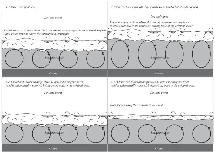
There are two hypotheses to be tested. These are that the clearing and consequent breaking up of the cloud is a result of the following:
1. Increased entrainment of dry air into the cloud layer, which reduces the total water content to levels below the saturation vapour mixing ratio at the initial altitude of the cloud level. This results in evaporation of the cloud when it descends to the original level.
Dry and warm
Ocean
Boundary layer
Entrainment of air from above the inversion serves to evaporate some cloud droplets. Total water remains above the saturation mixing ratio
1. Cloud at original level
Dry and warm
Ocean
Boundary layer
2. Cloud and inversion lifted by gravity wave (and adiabatically cooled)
Entrainment of air from above the inversion evaporates droplets - is total water below the saturation mixing ratio at the original level?
Dry and warm
Ocean
Boundary layer
3.a. Cloud and inversion drops down to below the original level (and is adiabatically warmed) before rising back to the original level.
Dry and warm
Ocean
Boundary layer Does the warming then evaporate the cloud?
3. b. Cloud and inversion drops down to below the original level (and is adiabatically warmed) before rising back to the original level.
Fig. 1.Schematic of the first hypothesis to be tested: does the cloud clear due to additional cloud-top entrainment as a result of the wave?
(1) Cloud is at its equilibrium level; (2) cloud and the inversion are lifted by the gravity wave, which results in higher liquid water contents due to cooling, entrainment causes increased evaporation relative to (1); (3) if the total water mixing ratio is still above the saturation vapour mixing ratio at the cloud’s equilibrium level, then the cloud will be maintained; (4) if the total water mixing ratio is below saturation, then the cloud will evaporate and clear and the air close to the inversion may decouple from fluxes of water below.
the air below and cutting off the boundary layer thermal and moisture circulation.
These processes are not necessarily independent and may both be in play; they are illustrated and explained in Figs. 1 and 2. It is hypothesised that enhanced entrainment occurs (as shown in Fig. 1) because of enhanced evaporation at the cloud top during entrainment events. The larger liquid wa-ter contents that are present in the crest of the wave result in more evaporative and radiative cooling, which enhances tur-bulence and mixing at cloud top. Both mechanisms appear to be plausible (indeed the second has been highlighted by previous studies), but it is important to understand which is the dominant mechanism so that if parameterisations are to be developed, they may take account of the relevant physics and thus be more realistic.
2 Background to the VOCALS study
The VOCALS project took place from 15 October to 15 November 2008 in the SEP to investigate the interactions be-tween land, sea and atmosphere with the aim of improving representation of processes in the region in both global and regional models. Detailed descriptions of the international ef-fort have been presented and discussed in the scientific liter-ature (e.g. Wood et al., 2011b,a; Allen et al., 2011) and so the details will not be repeated here; rather we will present an overview of the campaign and discuss the measurements relevant to this paper.
Dry and warm
Ocean
Boundary layer
Entrainment of air from above the inversion serves to evaporate some cloud droplets. Total water remains above the saturation mixing ratio
1. Cloud at original level
Dry and warm
Ocean
Boundary layer
2. Cloud and inversion lifted by gravity wave (and adiabatically cooled)
Additional condensation causes cloud drops to become larger colliding and coalescing to form rain
Dry and warm
Ocean
Boundary layer
Water is lost from the cloud and evaporating rain creates cold pools, cutting off closed cells and initiating more convection
3. Cloud and inversion drops down to below the original level (and is adiabatically warmed) before rising back to the original level.
Dry and warm
Ocean
Boundary layer Does this cause a transition to open cells?
4. Cloud and inversion drops down to below the original level (and is adiabatically warmed) before rising back to the original level.
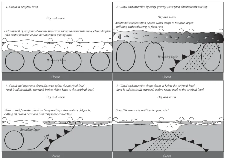
Fig. 2.Schematic of the second hypothesis to be tested: does the cloud clear due to drizzle forming and falling out? (1) Cloud is at its
equilibrium level; (2) cloud and the inversion are lifted by the gravity wave, which results in higher liquid water contents and drizzle formation, forming cold pools; (3) the boundary layer eddies are cut off by the cold pools and the cloud clears; (4) boundary cells form.
Allen et al. (2011) partitioned the VOCALS measurements into three regions, based on the location from the shore. These were coastal (to the east of 75◦W), transitional (be-tween 75◦W and 80◦W) and remote (to the west of 80◦W). They presented quad-log-normal fits to the median of the number–size distributions of aerosol particles measured in the MBL for each of these regions (these are shown in Ta-ble 1). The data show a clear trend of decreasing accumu-lation mode aerosol concentrations moving from the coastal to the remote region. Other statistics quantifying the region have been presented by Bretherton et al. (2010). Boundary layer height was∼1000 m close to the coast, increasing to ∼1500 m at 85◦W, whereas sea surface temperature (SST) increased to a maximum close to the coast (see Bretherton et al., 2010). These factors likely play a role in determining the location of POCs over the region, which tend to occur most frequently in the transition region and perhaps the re-mote region.
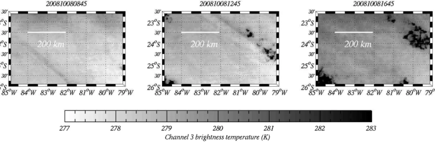
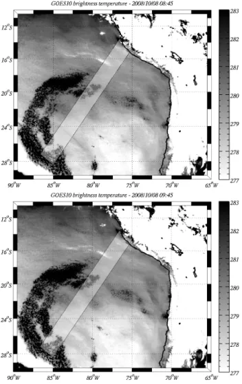
Figure 3 shows a case study that Allen et al. (2012) pre-sented of a gravity wave triggering the formation of POCs
within an area of otherwise overcast Sc. Throughout the day several gravity wave packets propagated in a north-east direction and eventually resulted in the cloud opening up (Fig. 3, centre) at 79 to 81◦W. This persisted and became more prevalent throughout the day (Fig. 3, right). The study will now focus on determining the mechanism that causes the cloud to clear.
3 Methodology
3.1 Large eddy modelling (LEM)
Version 2.4 of the UK Met. Office (Met. Office) large eddy model (LEM) (Gray et al., 2001) was used to simulate the in-teraction between dynamics, microphysics and radiation for an idealised case based on observations from the VOCALS campaign.
Fig. 3.GOES10 channel 3 brightness temperature imagery of gravity waves initiating POCs (Allen et al., 2012, adapted from). Left: bright-ness temperature observed at 08:45; centre: brightbright-ness temperature observed at 12:45; right: brightbright-ness temperature observed at 16:48. All times in the figure are GMT.
Table 1.Fit parameters to the measured aerosol size distributions observed during the VOCALS campaign. Reproduced following Allen
et al. (2011).
Mode Fit parameter Within the MBL
Coastal Transitional Remote
1 NL(cm−3) 20.065±0.009 13.278±0.803 46.642±1.730 log σg 0.435±0.000 0.260±0.019 0.348±0.015 Dm(µm) 0.014±4.740 0.013±0.000 0.018±0.000
2 NL(cm−3) 114.996±0.007 155.208±1.085 153.421±1.737 log σg 0.353±2.790 0.497±0.004 0.354±0.004 Dm(µm) 0.050±1.710 0.042±0.000 0.039±0.000
3 NL(cm−3) 268.099±0.008 175.766±1.017 166.774±1.992 log σg 0.444±1.704 0.429±0.002 0.465±0.006 Dm(µm) 0.157±3.272 0.158±0.000 0.154±0.001
4 NL(cm−3) 15.347±0.012 0.813±1.724 n/a log σg 0.310±0.000 0.350±0.860 n/a Dm(µm) 0.619±0.000 1.839±1.808 n/a
continuity is diagnosed via an elliptical equation and serves as a source term for momentum. The LEM explicitly resolves large-scale turbulent motions, which are responsible for most of the turbulent energy and transport, while parameterising sub-grid motions with a first-order turbulence scheme.
The majority of simulations presented use a vertical do-main extending from the surface to 3 km, while the horizontal domain is 16 km×16 km in extent. The horizontal resolution (1x,1y) is 120 m and the vertical resolution (1z) 20 m be-low the inversion. Starting 100 m above the inversion to an altitude of 2000 m the vertical grid spacing was stretched to 50 m. This results in a grid size of 128×128×105 points on which the solutions were computed. In Sect. 4.8 we assess whether our findings are sensitive to both domain size and grid resolution.
The initialisation time was 08:00 GMT, which is approx-imately 03:00 LT. The simulation time for all cases is 12 h with a variable time step to satisfy two separate Courant– Fredrichs–Lewy (CFL) criteria. The first criterion was that the Courant number, ∼u×1x1t ≤0.2, and the second was that the viscous stability parameter,∼41t ν
1x2 ≤0.2, whereν is the viscosity of the flow, the dependence of which has a parameterised relation to the resolved part of the flow. The maximum time step is limited to 5 s.
To initialise the model the vertical profiles of horizon-tal wind and geostrophic wind were set to a constant u= 7.0 m s−1andv= −1.0 m s−1. Geostrophic wind forcing is
required to maintain the horizontal winds, otherwise the effects of surface friction would reduce the wind speed throughout the simulation. The initial cloud liquid water con-tent was set to be adiabatic leading up to the inversion and specified to be horizontally homogeneous throughout the model, while the initial drop number concentration was set to be 100 mg−1of air. The total number of CCN was set to be 500 mg−1of air below the inversion and to zero above the in-version, which is consistent with the VOCALS region (Allen et al., 2011) for the purpose of a relative contrast between the MBL and free troposphere; however, there were episodes where pollution was transported large distances, resulting in discrete layers of higher CCN concentrations that may have been entrained into the MBL (this effect is not addressed in the current study).
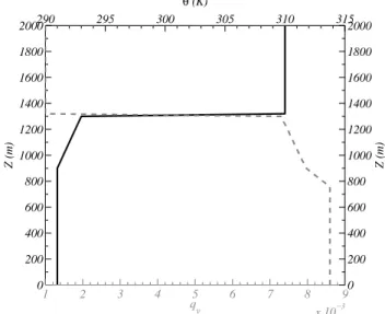
The potential temperature, θ, and vapour mixing ratio,
qv, were initialised with an idealised sounding as shown in
Fig. 4.
To promote turbulence a random perturbation with max-imum magnitude of ±0.1 K was applied to the initial po-tential temperature field below the inversion; no perturbation was added above the inversion. The model was also run with interactive shortwave and longwave radiation (Edwards and Slingo, 1996), which was updated every 150 s model time. Rather than use a set droplet effective radius for the radia-tive transfer scheme, it was diagnosed from the microphysics scheme, which allows the so-called “Twomey effect” to be accurately modelled. Large-scale divergence was specified to be 3×10⁻⁶s−1 , which is consistent with both QuikSCAT
and WRF simulations for the period in question (Rahn and Garreaud, 2010) and helps to maintain the inversion.
The microphysics scheme used was a two-moment scheme for both cloud water and rain water fields and based on that by Morrison et al. (2005), but with prognostic CCN. In accord with the in situ observations, the representation of the raindrop size distribution within the LEM microphysics scheme was parameterised as an exponential distribution. The rate of warm rain formation was parameterised using the auto-conversion scheme described by Seifert and Beheng (2006). This scheme requires that the cloud drop size distri-bution is input as a modified gamma distridistri-bution in mass and the rain drop distribution be exponentially distributed. Short-comings of assuming an exponential distribution for rain are acknowledged since, in reality, the larger drizzle drops tend to sediment out of the cloud, resulting in the drizzle hav-ing a well-defined “mode” rather than behav-ing exponentially distributed (Dearden et al., 2011), and the results here may prove to be sensitive to these assumptions.
In addition to the prognostic model fields for cloud drop number concentration and mass mixing ratio, a parameterisa-tion for the effective radius in stratocumulus clouds (Martin
290 295 300 305 310 315
0 200 400 600 800 1000 1200 1400 1600 1800 2000
Z (m)
θ (K)
1 2 3 4 5 6 7 8 9
x 10−3
0 200 400 600 800 1000 1200 1400 1600 1800 2000
q
v
Z (m)
Fig. 4.Initial potential temperature and vapour mixing ratio for the
model simulations presented.
et al., 1994) is used to enable the specification of all three pa-rameters in the modified gamma distribution for cloud water. The microphysics scheme also has a field for prognostic CCN, which interacts with the cloud fields, therefore hav-ing consistent sources and sinks. Observational data were used to constrain the CCN within the model as described in Sect. 3.1.2.
3.1.1 Gravity wave kinematics
The gravity wave properties were derived from GOES10 satellite observations of brightness temperature in the ther-mal infrared. The approximation was made that the bright-ness temperature was equal to the temperature of the top of the cloud and that the initial lifting (before precipitation oc-curred) was adiabatic. This allowed us to quantify the wave-length and amplitude of the gravity wave packet.
The observations showed that the wave was monochro-matic (Allen et al., 2012), and non-dispersive. Hence, the phase velocity,vp=ω
k, could be calculated using
consecu-tive images to see how far the wave crests travelled in a time period.
In order to do this we took two consecutive GOES10 satel-lite images, taken an hour apart, and drew a rectangular box perpendicular to the wave front. We then calculated means and standard deviations of the brightness temperatures as a function of distance perpendicular to the wave front. Figure 5 shows two GOES10 images that depict this procedure, with the rectangles showing the area over which statistics were taken.
Fig. 5.Gravity waves observed from GOES10 satellite data for im-ages taken at 08:45 and 09:45 GMT. The rectangles shown on each image depict the area over which the statistics of brightness temper-ature where calculated.
Allen et al. (2012) provided an estimate of the wavelength of ∼55 km, although our more rigorous analysis suggests that ∼100 km is a better characterisation. Comparing Fig. 6a and b it can be seen that the wave has moved around 55 km in distance from its original location at 08:45 GMT, hence the phase velocity of the wave,vp∼553600×103 ∼15.3 m s−1.
In order to convert the difference in brightness temperature to a displacement in altitude we assume that the wave lifting is adiabatic. At∼280 K the saturated adiabatic lapse rate is approximately 6 K km−1, and so this can be used to convert
the brightness temperatures to a displacement. Figure 6c and d suggest that the amplitude of the wave was around 50 to 100 m, at least for the period shown. In another case (not discussed here) the amplitude of the wave could extend to around 150 to 250 m.
Due to computational constraints, for the majority of runs, our model domain was only 16 km×16 km in the
horizon-tal. Figure 7 superimposes such a domain on a satellite im-age, showing it to be considerably smaller than the scale of convective organisation; thus we cannot aim to represent an MCC. Further, the domain is much smaller than the gravity wave wavelength (∼100 km), so we cannot model the pas-sage of the wave across the domain either. Rather, we restrict this study to an investigation of the physics leading to cloud clearing by applying a wave perturbation uniformly across the domain. This perturbation is generated by modulating the subsidence velocity in the model.
The properties of a time-dependent horizontally homoge-neous wave that this produces can be derived from the prop-erties of the travelling wave through the relation between phase velocity,vp, wave number,k=2πλ , and angular veloc-ity,ω=2π
T , i.e. vp=
ω k =
λ
T; (1)
therefore, we can derive the period of the equivalent time-dependent wave to be T = λ
vp ∼ 100×103
15.3 ∼6500 s. There
were slight variations in the derived time periods depending on the time of day and location; hence, an average value for the period of the wave, for use in the model, was taken to be
T =5400 s.
Adding this forcing produces an adiabatic cooling to the cloud, which the model microphysics and dynamics respond to. The requirement is that the amplitude at the inversion,A, is 150 m and that this decays to zero at the surface (to satisfy the gravity wave boundary condition). Thus we linearly in-creased the amplitude of the wave from zero at the surface to
Aat the height of the inversion:
z(z, t )=
z+Azz
i
sin2π[t−t0] T
ifz≤zi z+Asin2π[t−t0]
T
ifz > zi zift < t0ort > t0+n×T
. (2)
wherezis the altitude,t is time,zi is the height of the in-version,t0is the time when the wave starts,T is the period of the wave,nis the number of cycles of the wave that the cloud is subject to, andAis the wave amplitude. Differenti-ating Eq. (2) with regard to time yields the velocity
w(z, t )=
Az zi ×
2π T cos
2π[t−t0]
T
ifz≤zi A×2π
T cos
2π[
t−t0] T
ifz > zi
0 ift < t0ort > t0+n×T
, (3)
wherew is the vertical wind to be added to the subsidence forcing in the model.
The gravity wave therefore does not directly affect the small-scale dynamics within the Sc deck, but does so indi-rectly, through the inhomogeneities brought about by extra condensation and warm rain formation.
350 400 450 500 550 600 278
278.2 278.4 278.6 278.8 279 279.2
distance (km)
Brightness temp. (K)
(a) Brightness temp. perp. to wave @ 0845 UTC
350 400 450 500 550 600 278
278.2 278.4 278.6 278.8 279 279.2
distance (km)
Brightness temp. (K)
(b) Brightness temp. perp. to wave @ 0945 UTC
350 400 450 500 550 600−150 −100 −50 0 50 100 150
distance (km)
displacement (m)
(c) Vertical displacement @ 0845 UTC
350 400 450 500 550 600−150 −100 −50 0 50 100 150
distance (km)
displacement (m)
(d) Vertical displacement @ 0945 UTC
Fig. 6.Statistics of the gravity wave observed from GOES10 satellite data. (a)and (c)are the brightness temperatures and calculated
displacements for the left image in Fig. 5 respectively, while(b)and(d)are the same but for the right image in Fig. 5. The solid lines are means and the error bars depict 1 standard deviation, either side of the mean.
Fig. 7.Figure showing the scale of the model simulations. Left
shows the domain depicted on a satellite image of GOES10 bright-ness temperatures that extends 6–7◦in latitude and longitude, while the right image shows the domain depicted on a satellite image that extends 1◦in both latitude and longitude.
3.1.2 CCN activation and parcel modelling
The purpose of this section is to provide details on how observations were used to constrain the CCN inputs to the LEM. CCN activation within the LEM microphysics scheme used in this study follows the Twomey (1959) approach, where the number of CCN activated depends on the peak up-draft velocity at cloud base. In fact we used the more com-mon approximation found in Rogers and Yau (1989):
NCCN=0.88×C2/(2+k)×70×w3/2
(k/(2+k))
, (4)
whereNCCNis the drop concentration (cm−3) at cloud base, wthe updraught speed in m s−1andC(cm−3) andkare
con-stants describing the supersaturation activity of the CCN –
NCCN=Csk, wheresis the supersaturation in percent. This
approach requires the constantsCandk, which were derived by applying a parcel model (described below) to aerosol data taken from the BAe-146 FAAM aircraft measurements pre-sented in Allen et al. (2011).
Aerosol size distributions in the MBL over the SEP were measured on board the BAe-146 Facility for Airborne At-mospheric Measurements (FAAM) aircraft using an scanning mobility particle sizer (SMPS) and a passive cavity aerosol spectrometer probe (PCASP) as described by Allen et al. (2011). The chemical composition of the aerosol was mea-sured with a Aerodyne Aerosol Mass Spectrometer (AMS) and found to be predominantly sulfate internally mixed with a small amount of organics.
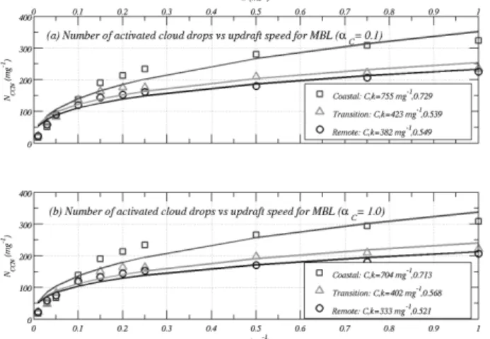
Fig. 8.Results from the parcel model simulating the number of ac-tivated cloud drops as a function of updraft velocity.(a)shows cal-culations when a mass accommodation coefficientαC=0.1 and(b) shows the same but forαC=1.0. In each case, squares are for the coastal region, triangles are the for transition region and circles for the remote region. Fitted values for the constantsCandkin Eq. (4) are shown in the legend.
determine the dependence of CCN number concentration on updraft speed. Following this, Eq. (4) was fitted to the model output, using non-linear regression, to find the constantsC
andk. This was repeated for each of the three regions de-scribed by Allen et al. (2011): coastal, transitional and re-mote. We also investigated the dependence of the results on the mass accommodation coefficient, αC, which is poorly
constrained at the present time, thus making a total of 60 runs for this analysis. The initial conditions for the ACPIM parcel modelling were pressure,P =950 mbar; temperature,
T =11◦C; and relative humidity, RH=0.95. The model was run for a total ascent of 200 m, at which point the number of activated cloud drops was determined.
The results of the ACPIM parcel modelling are shown in Fig. 8a and b, which shows only a small sensitivity toαCin the range 0.1≤αC≤1.0. As expected, the number of CCN decreases with increasing distance from the coast, although there is little drop-off in CCN concentrations when moving from the transition region to the remote region. In the context of this study the coastal CCN concentrations will be referred to as “high”, transitional will be referred to as “medium” and remote will be referred to as “low”. It is recognised that these CCN values do not represent a large variation in CCN number concentration; nevertheless, the descriptors, high, medium and low are relevant in the context of this study. All runs, unless explicitly stated, used medium CCN concentra-tions.
The LEM was used to investigate the effect of the imposed wave on the dynamics and microphysics of the stratocumu-lus clouds. A number of model runs based on the
methodol-Table 2. A summary of the sensitivity tests performed with the
LEM.
CNTRL Control simulation – no gravity wave, medium CCN GW150 Same as control, but with 150 m wave at 05:00 LT GW200 Same as control, but with 200 m wave at 05:00 LT GW250 Same as control, but with 250 m wave at 05:00 LT GW300 Same as control, but with 300 m wave at 05:00 LT GW150CCNL 150 m amplitude wave with low CCN
GW300CCNH 300 m amplitude wave with high
GW150x2 Same as control but with 2×150 m wave at 05:00 LT GW150x3 Same as control but with 3×150 m wave at 05:00 LT GW150x4 Same as control but with 4×150 m wave at 05:00 LT GW150x4 NR Same as GW150x4 and no warm rain
GW150 s3 Single 150 m wave occurring at 08:00 LT GW150 s4 Single 150 m wave occurring at 09:00 LT
ogy described in Sects. 3.1, 3.1.1 and above were performed, which, for completeness, are listed in Table 2.
4 Results – LEM simulations
Here we present results from the LEM simulations to show the sensitivity to the forcing imposed by gravity waves. The results are organised into eight main sections, dealing with the effects of the amplitude of the gravity waves on the re-sponse of the modelled MBL Sc; the effect of including multiple waves of amplitude,A=150 m; the effect of wave timing and the temporal evolution of the cloud, specifically waves occurring at night and during daytime; the effects of warm rain and CCN; and cloud-top entrainment and the grid spacing/domain size.
Firstly, we present images of the modelled LWP for two of the simulations: one without any imposed gravity wave forcing and one with a single 150 m amplitude gravity wave initiated at 05:00 LT. Figure 9 shows the results of these two simulations and shows that the effect of the wave is to firstly increase the LWP (Fig. 9a and e), following which the cloud clears and breaks up in the downward part of the wave (Fig. 9b and f). However, the LWP soon recovers almost to previous values (Fig. 9c and g), but then starts to break up towards the end of the simulation (Fig. 9d and h). Al-though there are similarities to the satellite images presented in Fig. 3, it is apparent that the modelled clouds take much longer to clear (some 8 h after the occurrence of the wave), whereas in the observations, clearance occurred almost im-mediately after the passage of the wave. The model results in this case are therefore not consistent with the observations.
4.1 Effect of wave amplitude
−5000 0 5000 −5000
0 5000
x (m)
y (m)
(a) no wave @ 05:15 local
−5000 0 5000
−5000 0 5000
x (m)
y (m)
(e) 150 m wave @ 05:15 local
−5000 0 5000
−5000 0 5000
x (m)
y (m)
(b) no wave @ 06:00 local
−5000 0 5000
−5000 0 5000
x (m)
y (m)
(f) 150 m wave @ 06:00 local
−5000 0 5000
−5000 0 5000
x (m)
y (m)
(c) no wave @ 08:30 local
−5000 0 5000
−5000 0 5000
x (m)
y (m)
(g) 150 m wave @ 08:30 local
−5000 0 5000
−5000 0 5000
x (m)
y (m)
(d) no wave @ 15:00 local
−5000 0 5000
−5000 0 5000
x (m)
y (m)
(h) 150 m wave @ 15:00 local
LWP (kg m−2)
1e−05 0.0001 0.001 0.01 0.1 1
Fig. 9.Snapshots of the LWP modelled for a case without an imposed gravity wave(a–d)and with an imposed gravity wave with amplitude,
A=150 m(e–h).(e)shows the cloud layer being lifted and the associated increase in LWP, whereas(f)shows the layer descended in the trough of the wave.(d)and(h)show that the effect of the wave is to break up the cloud layer.
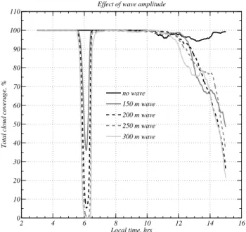
set of simulations. It is seen that the case without any grav-ity waves results in almost completely overcast conditions, whereas the cases with waves all result in a slow clearing of the cloud, some 8 h after the occurrence of the wave. While there are some subtleties, it is apparent in these simulations that wave amplitude does not have an appreciable effect on the clearing of the cloud. However, it is noteworthy that the 300 m wave results in the MBL Sc taking longer to fill in after the occurrence of the wave at∼06:50 LT. It may therefore be that waves with higher amplitudes than 300 m would result in a rapid clearing of the cloud; however, such high amplitudes were not observed and are deemed to be unrealistic.
4.2 Effect of multiple waves
It is clear from the GOES10 imagery that a gravity wave train can contain multiple peaks and troughs. Hence we decided to examine the sensitivity of the modelled MBL Sc to the number of gravity wave oscillations by including 1, 2, 3 or 4 successive cycles of the wave. Figure 11 shows a comparison of modelled LWP, comparing a case with no gravity waves to a case with 3 successive gravity waves. In this figure, pan-els (e), (f) and (g) show times in the downward moving part of the wave, and hence show the cloud breaking up after an
initial increase in LWP prior to this. When comparing these to the equivalent times without a gravity wave (a, b and c) it can be seen that each time a wave occurs, it results in an in-crease in the amount of broken cloud. Figure 11d and h show the cloud at the end of the model simulations, long after the waves occurred, where it is clear that the case with 4 waves has resulted in a significant amount of clearing of the cloud layer.
2 4 6 8 10 12 14 16 0
10 20 30 40 50 60 70 80 90 100 110
Local time, hrs
Total cloud coverage, %
Effect of wave amplitude
no wave 150 m wave
200 m wave 250 m wave
300 m wave
Fig. 10.Time series of the total cloud coverage from the LEM in
percent for gravity waves with different amplitudes,A. It is shown that the case without a gravity wave leads to overcast conditions, while all other cases lead to a reduction in cloud coverage – albeit some 8 h after the wave.
4.3 Effect of timing of the wave
To attempt to answer the question of whether the cumulative effect of multiple waves was important or whether it is the timing that is important we ran two simulations using single 150 m waves but altered the time of day at which they oc-curred: (i) the time at which the 3rd wave occurred in the 3-and 4-wave simulations “single 3rd wave” 3-and (ii) the time at which the 4th wave occurred in the 4-wave simulation “single 4th wave”. The LWP fields from these simulations are shown in Fig. 13. Figure 13a and e show the LWP before any grav-ity wave perturbations have been applied, whereas Fig. 13b shows a time just after the wave in the single 3rd wave sim-ulation; Fig. 13f is the same time but for the single 4th wave simulation. Figure 13g shows the LWP field at a time just af-ter the wave in the single 4th wave simulation. By this time both simulations display broken cloud, the amount of which increases towards the end of the simulation (Fig. 13d and h). Thus here it is apparent that the timing of the wave is crucial to its effect on the MBL Sc.
The results of the simulations shown in Fig. 13 are com-pared to the “no wave” case and summarised in terms of total cloud cover in Fig. 14. Here it is apparent that the single 3rd wave simulation does not result in a dramatic reduction in to-tal cloud cover, but it does take time to fill back in to 100 %, before breaking up again in a similar way to all single-wave cases. However the single 4th wave case does result in a clear reduction in cloud coverage, although not quite as dramatic
as the case that included four cycles of the wave. There is no strong evidence for a change in convective regime, like in Fig. 12. It is therefore apparent that both the timing and the number of waves affect cloud clearing. A point worth not-ing is that there was more drizzle in the case with multiple waves, and this had an impact on the development of weak cold pools in the MBL, which increased convective instabil-ity.
Figures 14 and 15a suggest that at 09:00 LT the boundary layer is still strongly coupled to the surface fluxes of mois-ture; this is why the single 3rd wave case does not result in a clearing of the cloud layer. However, by approximately 11:00 LT (or just after) it appears that the boundary layer becomes decoupled from the moisture fluxes. The decoupling of the cloud layer from the lower level fluxes may be demonstrated by a vertical profile of the variance of vertical velocity,w′w′.
Figure 15a and b show the variance of the vertical veloc-ity for five model simulations: the no wave case, the single 1st wave case, the case with 4150 m waves and the single 3rd wave and single 4th wave case. Figure 15a shows the variance of vertical velocity at 09:00 LT showing thatw′w′
is reasonably high in the cloud region for all cases except the simulation with 4 wave cycles. It should be noted that at 09:00 LT in both the simulation with 4 wave cycles and the single 3rd wave case wave subsidence is occurring, which effectively lowers the inversion by 150 m.
Figure 15b shows the corresponding variance of vertical velocity at 12:00 LT and shows a significant reduction in the velocity variance for all simulations, with a weighting towards higher variances near the surface, thus signalling the decoupling of the cloud from the surface fluxes. It is notice-able that both the simulation with 4 waves and the single 4th wave case have lower variance of vertical velocity in the re-gion 600< Z <1200 m than the other cases at this time. Al-though not shown here, analysis of the variance of vertical velocity at the end of the simulations shows that, of all of the simulations, the case with 4 waves leads to the highest vari-ances throughout the depth of the boundary layer. Although this demonstrates some degree of coupling, it is not homo-geneous across the model domain and is more similar to Cu type convection.
4.4 Evolution of cloud throughout the day
−5000 0 5000 −5000
0 5000
x (m)
y (m)
(a) no wave @ 07:15 local
−5000 0 5000
−5000 0 5000
x (m)
y (m)
(e) 4x150 m waves @ 07:15
−5000 0 5000
−5000 0 5000
x (m)
y (m)
(b) no wave @ 08:45 local
−5000 0 5000
−5000 0 5000
x (m)
y (m)
(f) 4x150 m waves @ 08:45
−5000 0 5000
−5000 0 5000
x (m)
y (m)
(c) no wave @ 10:15 local
−5000 0 5000
−5000 0 5000
x (m)
y (m)
(g) 4x150 m waves @ 10:15
−5000 0 5000
−5000 0 5000
x (m)
y (m)
(d) no wave @ 15:00 local
−5000 0 5000
−5000 0 5000
x (m)
y (m)
(h) 4x150 m waves @ 15:00
LWP (kg m−2)
1e−05 0.0001 0.001 0.01 0.1 1
Fig. 11.Same as Fig. 9 except the comparison is for no wave vs. 4 successive gravity waves with amplitude,A=150 m. The cases with 4
successive waves are shown in(e–h).(e–g)show conditions in the downward part of the last 3 waves respectively, whereas(h)shows the end of the simulation.
It is shown that cloud-top altitude after the single 3rd wave and single 4th wave simulations is lower than the no wave case. This is similar for the cloud-base altitude. In both cases the difference is considerably greater than in the single 1st wave case. The lowering of the cloud top is an indicator of cloud-top entrainment; hence, these results suggest that there is not much enhancement of cloud-top entrainment in the sin-gle 1st wave case. This is a qualitative demonstration that entrainment is enhanced in the cases with imposed gravity waves and that the timing of the wave is crucial to the effect that cloud-top entrainment has on the evolution of the cloud.
4.5 Effect of warm rain formation
The importance of multiple successive waves may suggest that each time the cloud layer is lifted, the resulting warm rain acts to reduce the LWP resulting in a cumulative ef-fect on the clearing of the cloud. Warm rain generation was indeed seen in the model fields each time the cloud layer was lifted; however, this rarely reached the surface in the model, as it evaporated during its descent. In order to ascer-tain the importance of the warm rain process we ran an addi-tional model simulation with the warm rain auto-conversion scheme switched off for the case with 4 successive waves.
The results of this are summarised in Fig. 17. Here it can be seen that both cases result in a clearing of the MBL Sc, there-fore suggesting that the main process responsible for clearing the cloud is not the warm rain process itself. However, we note that the simulation with warm rain results in a change in convective regime later in the simulations (as shown by the more rapid increase in total cloud coverage near the end of the simulation). Other analyses of the variance of vertical velocity (not shown) indicate that the “4×150 m wave” case with rain has much higher variances in the cloud layer at the end of the simulations compared to the same case without warm rain. The reason for this is that the evaporation of rain below cloud destabilises the boundary layer so that the cloud layer has better coupling to the surface fluxes of moisture. Also worthy of note is that the simulation with warm rain re-sults in the lowest cloud coverage in each downward part of the wave, which is as expected since warm rain removes total water from the cloud layer.
4.6 Influence of CCN concentration
2 4 6 8 10 12 14 16 0
10 20 30 40 50 60 70 80 90 100 110
Local time, hrs
Total cloud coverage, %
Effect of wave number of waves
no wave 150 m wave
2x150 m wave 3x150 m wave
4x150 m wave
Fig. 12.Similar to Fig. 10 but comparing the effect of different
num-bers of gravity wave. It is seen that the cases with both 3 and 4 waves lead to a dramatic reduction in total cloud coverage.
CCN concentrations for all three regions are described in Sect. 3.1.2 and shown in Fig. 8. To investigate the role of CCN, two additional simulations were performed, both in-cluding warm rain processes. One was a 300 m wave with high CCN and the other was a 150 m wave with low CCN. These were chosen to demonstrate whether (i) high CCN could suppress the slow clearing of the cloud that occurred 8 h after the wave (Fig. 10) and whether (ii) low CCN could lead to additional clearing of the cloud due to warm rain.
Figure 18 (top) shows the time series of total cloud cover for these simulations. The results show that the 300 m wave with high CCN results in a cloud with almost 100 % cloud coverage. This is in contrast to the simulation with a 300 m wave (and medium CCN), which resulted in a clearing of the cloud. The reason for this is that the case with higher CCN re-sulted in more cloud-top radiative cooling (because the cloud droplets were smaller and more numerous), an effect that was able to maintain the cloud coverage at higher values due to additional condensation.
The simulation with a 150 m wave and low CCN failed to clear the cloud. More warm rain was produced in this case than the simulation with a 150 m wave and medium CCN, which resulted in lower cloud coverage at 11:00 LT; however, the cloud coverage then recovered, presumably because this moistened and cooled the air below the cloud and resulted in a more coupled boundary layer. Hence, it appears that CCN do play an important role in the clearing of the cloud. The in-termediate CCN values away from the coast are more likely to result in a clearing of the cloud than both the higher CCN values close to the coast and the lower CCN values away
from the coast. Although the CCN variability within the VO-CALS dataset was higher than that taken from comparing the means from the three regions (coastal, transitional and remote), it is encouraging that use of observationally con-strained CCN within the LEM is able to provide insights into some of the reasons why the clearing of cloud occurs prefer-entially in the transition region. It is also likely that bound-ary layer height plays an important role in the clearing of the cloud; however, this effect is not investigated here.
Figure 18 (bottom) shows the time series of the domain-averaged LWP for the CCN simulations. It can be seen that LWP increases during the crest of the wave, decreases during the trough and then increases to values that are below those seen in the no wave case. Also evident is that higher CCN results in higher LWPinitially, but later in the simulations the opposite is true (e.g. compare “150 m wave” with “150 m wave low aerosol” and “300 m wave” with “300 m wave high aerosol”).
4.7 Effect of cloud-top entrainment
In order to probe whether entrainment of dry air from aloft may be responsible for cloud clearance, we initialised a pas-sive tracer in the model, set to 1.0 above the inversion and zero below the inversion (Fig. 19a). Figure 19b shows the horizontal mean of the tracer field in the model at 12:00 LT. This shows some mixing of the tracer from above the inver-sion into the boundary layer for all model runs.
Interestingly, the run with one 150 m gravity wave occur-ring early in the morning has a tracer distribution that is al-most the same as the case without any wave; hence the sin-gle, early gravity wave does not cause any additional mixing. When 4×150 m waves are used for the forcing, there is much more mixing of air above the inversion into the cloud layer. In addition, a similar effect happens when we use a single 150 m gravity wave that occurs later in the day (single 4th wave). Therefore, the tracer results suggest that it is the mix-ing in to the cloud of warm, dry air from above the inversion that causes the rapid evaporation of the cloud shortly after the wave. The eddies responsible for the mixing of dry air into the cloud were resolved in the model wind field, as can be seen in the variance of the vertical velocity (Fig. 15), and were a result of latent heating creating more energetic ther-mals that were able to break through the inversion.
4.8 Effect of grid spacing and domain size
−5000 0 5000 −5000
0 5000
x (m)
y (m)
(a) wave (time of 3rd) @ 07:15
−5000 0 5000
−5000 0 5000
x (m)
y (m)
(e) wave (time of 4th) @ 07:15
−5000 0 5000
−5000 0 5000
x (m)
y (m)
(b) wave (time of 3rd) @ 08:45
−5000 0 5000
−5000 0 5000
x (m)
y (m)
(f) wave (time of 4th) @ 08:45
−5000 0 5000
−5000 0 5000
x (m)
y (m)
(c) wave (time of 3rd) @ 10:15
−5000 0 5000
−5000 0 5000
x (m)
y (m)
(g) wave (time of 4th) @ 10:15
−5000 0 5000
−5000 0 5000
x (m)
y (m)
(d) wave (time of 3rd) @ 15:00
−5000 0 5000
−5000 0 5000
x (m)
y (m)
(h) wave (time of 4th) @ 15:00
LWP (kg m−2)
1e−05 0.0001 0.001 0.01 0.1 1
Fig. 13.Same as Fig. 9 except the comparison is for a single 150 m amplitude wave occurring before sunrise vs. a single 150 m gravity wave
with the same amplitude occurring at the same time as the last wave in the 4×gravity wave case.
2 4 6 8 10 12 14 16
0 10 20 30 40 50 60 70 80 90 100 110
Local time, hrs
Total cloud coverage, %
Effect of timing of the wave
no wave
150 m wave @ time of 3rd wave 150 m wave @ time of 4th wave
Fig. 14.Similar to Fig. 10 but comparing the effect of waves
occur-ring later in the day. It can be seen that the later the wave occurs the more dramatic the clearing of the cloud layer is.
150 m wave occurring at the time of the 4th wave (single 4th wave).
Figure 20a–c show the LWP for the high-resolution runs both before and after the gravity wave. It is clear that the cloud coverage is reduced most in the case with the grav-ity wave, a result that is consistent with the lower-resolution simulations (Fig. 13e–h). This consistency is further demon-strated by the total cloud cover (Fig. 21). It is notable that the amount of clearing taking place after the gravity wave (Fig. 21 grey solid line) is indeed slightly lower for the high-resolution case than the control (Fig. 14, black dashed line), suggesting that the entrainment rate is indeed lower in the high-resolution case. Nevertheless, the same effects are still evident in these high-resolution cases.
Feingold et al. (2010) demonstrated that cloud variability results from interactions between cellularisation, precipita-tion and mesoscale circulaprecipita-tions. To test whether our results are sensitive to the choice of domain size, we performed an additional two simulations: one without a gravity wave and one with a gravity wave occurring at the time of the 4th wave (single 4th wave). Each of the large-domain runs had
0 0.05 0.1 0.15 0
200 400 600 800 1000 1200 1400 1600 1800 2000
w’w’ (m2 s−2)
Z (m)
(a) Time=9:00 (coupled BL)
0 0.05 0.1 0.15 0
200 400 600 800 1000 1200 1400 1600 1800 2000
w’w’ (m2 s−2)
Z (m)
(b) Time=12:00 (decoupled BL)
no wave 150 m wave 4x150 m waves
150 m @ time of 3rd wave 150 m @ time of 4th wave
Fig. 15.Variance of vertical velocity throughout the model domain in simulations with no wave; four consecutive cycles of a 150 m wave
“4×150 m waves” a 150 m wave occurring at different times (“150 m wave”; “150 m wave @ time of 3rd wave” and “150 m wave @ time of 4th wave”).(a)shows the variance at 09:00 LT and(b)shows it at approximately 12:00 LT.
2 4 6 8 10 12 14 16
0 200 400 600 800 1000 1200 1400 1600 1800 2000
Local time, hrs
Altitude (m)
Effect of timing of the wave
no wave
150 m wave @ time of 1st wave
150 m wave @ time of 3rd wave 150 m wave @ time of 4th wave
Fig. 16.Shows the evolution of average cloud-top and cloud-base
heights for a simulation with no wave and three simulations with a 150 m wave that occurred at the time of the 1st, 3rd and 4th wave in the 4-wave simulation: single 1st wave, single 3rd wave and single 4th wave respectively.
it is demonstrated that the case with a gravity wave clears the cloud more effectively than the case without. However, it is evident that the case without a gravity wave also leads to sig-nificant cloud clearance (Fig. 20e).
2 4 6 8 10 12 14 16
0 10 20 30 40 50 60 70 80 90 100 110
Local time, hrs
Total cloud coverage, %
Effect of warm rain
no wave 4x150 m wave
4x150 m wave without warm rain
Fig. 17.Similar to Fig. 10, but comparing the effect of having warm
rain switch on or off in the model microphysics scheme. Very little difference is evident.
2 4 6 8 10 12 14 16 0
10 20 30 40 50 60 70 80 90 100 110
Local time, hrs
Total cloud coverage, %
Effect of CCN
no wave 150 m wave
300 m wave 150 m wave low aerosol
300 m wave high aerosol
2 4 6 8 10 12 14 16
0 0.05 0.1 0.15 0.2 0.25 0.3 0.35 0.4 0.45 0.5
Local time, hrs
Average LWP (kg m
−2
)
Effect of CCN
no wave 150 m wave 300 m wave 150 m wave low aerosol
300 m wave high aerosol
Fig. 18.Top: similar to Fig. 10 but looking at the effect of
hav-ing low or high CCN. In the 300 m amplitude wave it is shown that high CCN suppresses the clearing of the cloud. It is also true that low CCN suppresses the clearing of the cloud in the case of the 150 m amplitude wave. Bottom: plot shows the corresponding domain-averaged LWP.
Feingold et al. (2010); hence, domain size is important to the findings. Nevertheless, the model shows that this clear-ance occurs over several hours, whereas for the case with the gravity wave the reduction in cloud coverage is coincident with the wave. This rapid clearing after the gravity wave is consistent with the satellite observations.
5 Discussion
The model results suggest that gravity waves are able to re-sult in a rapid clearing of the cloud only when they occur after sunrise. In the simulations presented, this is likely re-lated to the fact that the Sc starts to become decoupled after sunrise. Decoupling of the boundary layer was a common oc-currence away from the coastal region during the VOCALS campaign (Jones et al., 2011), even in the mid-morning, be-fore solar insolation leads to stronger decoupling; however, despite the decoupling there was still often 100 % cloud cover.
In our simulations, when there is strong coupling between the sea and the cloud-topped boundary layer, gravity waves do not cause arapidclearing of the cloud, as the fluxes of wa-ter vapour from the ocean surface are sufficient to promote condensation and fill in the cloud, thus restoring the long-wave cooling that drives the turbulence within the boundary layer.
However, when gravity waves were specified to occur in Sc that were less strongly coupled, they did result in arapid
clearing of the cloud. The decoupled cloud was more patchy in appearance and therefore, after lifting, cloud-top entrain-ment was enhanced by horizontal gradients in evaporation, reducing the total water mixing ratio. After the ascent the majority of the cloud evaporated in the trough of the gravity wave due to adiabatic warming, which suppresses radiative cooling of the boundary layer air by virtue of increased short-wave heating and reduced longshort-wave cooling, thus reducing the LWP further. Since the cloud is less strongly coupled to the surface, the flux of water vapour is insufficient to replen-ish the cloud.
For gravity waves that occurred in a strongly coupled Sc the clearing of the cloud occurred over a much longer timescale (if at all), and was much slower. In this case the lifting caused by the gravity wave resulted in an increase in warm rain formation, which after precipitating out of the cloud resulted in a Sc with lower LWP, but still with 100 % cloud coverage. The slow clearing of the cloud that some-times occurred in these cases was due to the warming of the boundary layer throughout the day, and the associated increase in saturation vapour mixing ratio.
Hence, in the morning, strong coupling between the sur-face and cloud layer renders the effect of the gravity wave minimal as the surface fluxes suppress drying of the cloud by entrainment and radiative heating. However, when the cloud decouples, the extra LWP during the upward cycle of the gravity wave leads to an enhanced entrainment, which mixes in more dry air. This effect is not compensated by surface fluxes as the cloud is decoupled, and therefore the result is that the cloud clears.
0 0.2 0.4 0.6 0.8 1 1.2 0
200 400 600 800 1000 1200 1400 1600 1800 2000
tracer field
Z (m)
(a) Time=3:00 (start)
0 0.2 0.4 0.6 0.8 1 1.20
200 400 600 800 1000 1200 1400 1600 1800 2000
tracer field
Z (m)
(b) Time=12:00
no wave 150 m wave
4x150 m waves
150 m @ time of 4th wave
Fig. 19. (a)shows the initial concentration of a passive tracer that was set up to look at air entraining from above the inversion;(b)shows the
concentration of the tracer 9 h into the simulation for cases without a wave, with a 150 m wave occurring early in the morning, for 4×150 m amplitude waves and for a single 150 m wave occurring at the same time as the last wave in the 4×case.
clearing only occurred when CCN concentrations were spec-ified to be medium. However, it is noted that, in reality, CCN variability may be significant across all three regions; there-fore, using averages for each of these regions may not give a completely accurate picture. Nevertheless, it does give some useful insights into the processes that cause the cloud to clear. Wang et al. (2010) investigated aerosol perturbations on the generation of POCs using ∼100 km2-scale model simula-tions at 300 m horizontal resolution, finding that gradients in aerosol were indeed significant in promoting the develop-ment of POCs. This effect has not been investigated here.
The effect that CCN concentrations and warm-rain for-mation has on LWP in the simulations is notable. Here it is shown that initially the LWP is lower in the runs with lower CCN concentrations, as might be expected because, for a given LWP, lower drop concentrations lead to faster rain formation; however, later in the simulations the oppo-site was true. Such findings highlight the non-linearity of aerosol–cloud interactions.
Other reasons that the clearing is observed preferentially at distances away from the coast may be due to boundary layer depth, which increases with distance away from the coast, or SST, which decreases a short distance from the coast and then starts to increase with distance into the transition zone (see Bretherton et al., 2010). However, investigating these effects is outside of the scope of this study.
The question of whether clearing of the cloud will lead to the formation of POCs is difficult to answer with the cur-rent set of simulations as the domain size is not large enough to model mesoscale circulations and their self-organisation. Nevertheless, the simulation with four gravity waves dis-played an increase in turbulence after the cloud cleared, due to drizzle evaporating and causing cold pools; this led to a cloud layer that was more strongly coupled to the surface moisture fluxes towards the end of the simulation. Cold pools have been shown to be important components of open MCC circulations in an aircraft case study during the same project (Wood et al., 2011a). Our results support the finding of Wood et al. (2011a), who suggest that warm rain is not a sufficient condition for the formation of POCs, since at least in our simulations the clearing of the cloud occurs by mixing in of dry air, with cold pools serving to reinvigorate Cu-like con-vection.
6 Conclusions
The conclusions drawn from the study are as follows:
Fig. 20.Snapshots of liquid water path for high-resolution runs(a–c)and for large-domain runs with the same resolution as the control(d–f).
(a),(b),(d)and(e)are runs without gravity waves, whereas(c)and(f)are liquid water paths for runs with a single gravity wave occurring at the time of the 4th wave.
– Within the simulations presented, it was a combination of the entrainment of dry air from above the inversion and a reduction in longwave cooling that was responsi-ble for the rapid clearing of the cloud after the gravity wave occurred.
– Warm rain was important to reinvigorating cumulus clouds following the clearing of the Sc. This was be-cause the rain evaporated and resulted in colder air in the MBL, which displaced the warmer air and resulted in greater convective instability.
– Using transition or “medium” CCN values was impor-tant to simulate the slow clearing of the cloud that oc-curred towards the end of the simulation. Coastal or “high” CCN was able to suppress the clearing of the cloud because of cloud-top radiative cooling, which is consistent with observations of fewer POCs in the “coastal” region. Remote or “low” CCN also suppressed the clearing over the day because it resulted in a more coupled cloud.
– Using multiple waves to force the simulation resulted in a more dramatic clearing of the cloud, similar to that observed. Timing of the waves needs to be later in the day (after sunrise) for rapid clearing of the cloud.
– It appears that both hypotheses are true to an extent. The evidence presented from the model is that entrainment of dry air from aloft occurs where there is a rapid clear-ing of the cloud shortly after the gravity wave; however, warm rain may play a role in the transition to open cellu-lar convection through the generation of cold pools that result in increased convective instability.
2 4 6 8 10 12 14 16 0
10 20 30 40 50 60 70 80 90 100 110
Effect of resolution and domain size
Local time, hrs
Total cloud coverage, %
no wave−high res
150 m wave @ time of 4th wave−high res no wave−large domain
150 m wave @ time of 4th wave−large domain
Fig. 21.Total cloud coverage for the high-resolution and the
large-domain runs, both with and without gravity waves. Solid lines are for the high-resolution run and dashed lines are for the large-domain run. Black lines are runs without a gravity wave, and grey lines are runs with a single gravity wave at the time of the 4th wave.
Acknowledgements. We would especially like to acknowledge
Paul Williams and his colleagues at the Manchester FGAM who provided the in situ aerosol measurements and for their particular care and attention to the quality control and assurance of these data products. We would like to acknowledge the pilots of the BAe-146 aircraft. Funding from NERC is acknowledged for the VOCALS project under the grant code NE/F019874/1. Acknowledgement is also given to Dr. Dave Topping (University of Manchester/National Centre for Atmospheric Science) who provided the thermodynamic data for the aerosol so that the CCN properties could be predicted.
Edited by: R. Wood
References
Agee, E. N.: Observations from space and thermal convection: a his-torical perspective, B. Am. Meteorol. Soc., 65, 938–949, 1984. Albrecht, B. A.: Aerosols, cloud microphysics and fractional
cloudiness, Science, 245, 1227–1230, 1989.
Allen, G., Coe, H., Clarke, A., Bretherton, C., Wood, R., Abel, S. J., Barrett, P., Brown, P., George, R., Freitag, S., McNaughton, C., Howell, S., Shank, L., Kapustin, V., Brekhovskikh, V., Klein-man, L., Lee, Y.-N., Springston, S., Toniazzo, T., Krejci, R., Fochesatto, J., Shaw, G., Krecl, P., Brooks, B., McMeeking, G., Bower, K. N., Williams, P. I., Crosier, J., Crawford, I., Connolly, P., Allan, J. D., Covert, D., Bandy, A. R., Russell, L. M., Trem-bath, J., Bart, M., McQuaid, J. B., Wang, J., and Chand, D.: South East Pacific atmospheric composition and variability sam-pled along 20◦S during VOCALS-REx, Atmos. Chem. Phys., 11, 5237–5262, doi:10.5194/acp-11-5237-2011, 2011.
Allen, G., Vaughan, G., Toniazzo, T., Coe, H., Connolly, P. J., Yuter, S., Burleyson, C. D., Minnis, P., and Ayers, J. K.: Gravity-wave-induced pertubations in marine stratocumulus, Q. J. Roy. Meteo-rol. Soc., 139, 32–45, doi:10.1002/qj1952, 2012.
Berner, A. H., Bretherton, C. S., and Wood, R.: Large-eddy simu-lation of mesoscale dynamics and entrainment around a pocket of open cells observed in VOCALS-REx RF06, Atmos. Chem. Phys., 11, 10525–10540, doi:10.5194/acp-11-10525-2011, 2011. Bretherton, C. S., Macvean, M. K., Bechtold, P., Chlond, A., Cot-ton, W. R., Cuxart, J., Cuijpers, H., Khairoutdinov, M., Kosovic, B., Lewellen, D. C., Moeng, C. H., Siebesma, A. P., Stevens, B., Stevens, D. E., Sykes, I., and Wyant, M. C.: An intercompari-son of radiatively driven entrainment and turbulence in a smoke cloud, as simulated by different numerical models, Q. J. Roy. Meteorol. Soc., 125, 391–423, 1999.
Bretherton, C. S., Uttal, T., Fairall, C. W., Yuter, S., Weller, R., Baumgardner, D., Comstock, K., Wood, R., and Raga, G.: The EPIC 2001 stratocumulus study, B. Am. Meteorol. Soc., 85, 967– 977, 2004.
Bretherton, C. S., Wood, R., George, R. C., Leon, D., Allen, G., and Zheng, X.: Southeast Pacific stratocumulus clouds, precip-itation and boundary layer structure sample along 20◦S during VOCALS-REx, 10, 10639–10654, 2010.
Connolly, P. J., M¨ohler, O., Field, P. R., Saathoff, H., Burgess, R., Choularton, T., and Gallagher, M.: Studies of heterogeneous freezing by three different desert dust samples, Atmos. Chem. Phys., 9, 2805–2824, doi:10.5194/acp-9-2805-2009, 2009. Connolly, P. J., Emersic, C., and Field, P. R.: A laboratory
in-vestigation into the aggregation efficiency of small ice crystals, Atmos. Chem. Phys., 12, 2055–2076, doi:10.5194/acp-12-2055-2012, 2012.
Dearden, C., Connolly, P. J., Choularton, T. W., and Field, P. R.: Evaluating the effects of microphysical complexity in idealised simulations of trade wind cumulus using the Factorial Method, Atmos. Chem. Phys., 11, 2729–2746, doi:10.5194/acp-11-2729-2011, 2011.
Edwards, J. M. and Slingo, A.: Studies with a flexible new radiation code. Part I. Choosing a configuration for a large scale model, Q. J. Roy. Meteorol. Soc., 122, 689–719, 1996.
Feingold, G., Koren, I., Wang, H., Xue, H., and Brewer, W. A.: Precipitation-generated oscillations in open cellular cloud fields, Nature, 466, 849–852, 2010.
Garay, M. J., Davies, R., Averill, C., and Westphal, J. A.: Actino-form clouds. Overlooked examples of cloud self-organization at the mesoscale, B. Am. Meteorol. Soc., 85, 1585–1594, 2004. Garreaud, R. D. and Mu˜noz, R. C.: The Diurnal Cycle in
Circu-lation and Cloudiness over the Subtropical Southeast Pacific: A Modeling Study, J. Climate, 17, 1699–1710, 2004.
Gray, M. E. B., Petch, J. C., Derbyshire, S. H., Brown, A. R., Lock, A. P., Swann, H. A., and Brown, P. R. A.: Version 2.3 of the Met Office Large Eddy Model: Part II. Scientific Documentation, Tech. rep., 2001.
Hubert, L. F.: Mesoscale cellular convection, Tech. rep., 1966. Jiang, Q. and Wang, S.: Impact of Gravity Waves on Marine
Stra-tocumulus Variability, J. Atmos. Sci., 69, 3634–3652, 2012. Jones, C. R., Bretherton, C. S., and Leon, D.: Coupled vs.