Nonlinear Processes
in Geophysics
c
European Geosciences Union 2003
Geometric aspects of HF driven Langmuir turbulence in the
ionosphere
E. Mjølhus1, E. Helmersen2, and D. F. DuBois3
1University of Tromsø, Faculty of Science, Department of Mathematics and Statistics, N-9037 Tromsø, Norway 2Poseidon Simulation AS, N-8376 Leknes, Norway
3Los Alamos National Laboratory, Los Alamos, NM 87545, USA
Received: 24 September 2001 – Revised: 25 February 2002 – Accepted: 5 April 2002
Abstract.The geometric aspects of HF-generated Langmuir turbulence in the ionosphere and its detection by radars are theoretically discussed in a broad approach, including local modelling (damped and driven Zakharov system), basic para-metric instabilities, polarization and strength of the driving electric field, and radar configurations. Selected examples of numerical results from the local model are presented and discussed in relation to recent experiments, with emphasis on recent experiments at the EISCAT facilities. Anisotropic as-pects of the cavitation process in the magnetized plasma are exhibited. Basic processes of cascades and cavitation are by now well identified in these experiments, but a few problems of the detailed agreement between theory and experiments are pointed out.
1 Introduction
The outdoor experimental studies of parametric instabilities in a plasma, by transmitting powerful HF radio waves into the ionosphere and using VHF and UHF radars as diagnos-tics, started long ago (Carlson et al., 1972; Wong and Tay-lor, 1971). Experimental configurations have, up until re-cently, been in active use at Arecibo, Puerto Rico, and since the early 1980s at EISCAT, northern Scandinavia (Hagfors et al., 1983). Since about 1988, there has been a remarkable development of experimental techniques, leading to options of space-and time-resolved experiments with simultaneously high spectral resolution (Djuth et al., 1990; Fejer et al., 1991; Sulzer and Fejer, 1994; Kohl and Rietveld, 1996; Rietveld et al., 2000; Cheung et al., 2001; Djuth et al., 2002). This has allowed for a detailed comparison between experiments and theoretical predictions.
These studies may be said to occupy a position between controlled laboratory experiments and geophysical observa-tions. DuBois et al. (1996) discuss connections between these experiments and studies of parametric processes occur-Correspondence to:E. Mjølhus ([email protected])
ring in laser experiments. In the addition, these studies may open the road to using radars in studies of naturally occurring Langmuir turbulence in the ionosphere (Forme, 1999).
Early saturation theory was based on weak turbulence for-malism (Perkins et al., 1974; Fejer and Kuo, 1973; Rypdal and Craigin, 1979; Das et al., 1985). Recent theoretical ef-forts have been based on numerical solutions to full wave models of the Zakharov type with damping and parametric drive included (Nicholson et al., 1984; DuBois et al., 1990, 1991; Hanssen et al., 1992; Hanssen, 1992; Sprague and Fe-jer, 1995; DuBois et al., 1993a, 2001). This allows for the inclusion of phenomena not describable in weak turbulence theory (e.g. cavitation) and also for a more precise descrip-tion of the phenomena that weak turbulence theory includes, such as cascading.
A main issue of debate in the early stage of the period after 1988 was the mutual role of cavitation and cascade (Stubbe et al., 1992a, b; DuBois et al., 1992). Theoretically, a picture emerged (Hanssen et al., 1992; DuBois et al., 1993a, 2001) that cascading was to be expected in most of the height range below the O-mode reflection height, but that near the reflec-tion height, Langmuir cavitareflec-tion was to be expected. Predic-tions of radar spectral features resulting from the numerical studies (DuBois et al., 1988, 1990; Hanssen et al., 1992), were confirmed qualitatively in experiments at Arecibo (Fe-jer et al., 1991; Sulzer and Fe(Fe-jer, 1994; Cheung et al., 1989, 1992, 2001) and later also at Tromsø (Kohl and Rietveld, 1996; Isham et al., 1999b; Rietveld et al., 2000; Djuth et al., 2002), thus, strongly supporting the existence of Langmuir cavitation in these experiments.
is relevant for the case of the Arecibo experiments; in the EISCAT experiments other polarizations must also be con-sidered.
The present paper is devoted to two main issues which are somewhat interrelated: (i) numerical results will be presented for the first time for the case when the electric field polariza-tion is off-parallel , and (ii) more generally, the radar observ-ability of the HF driven Langmuir turbulence will be a cen-tral issue. The latter is connected to the relation between the directions of the radar line of sight and the electric field po-larization. The appropriate 2D driven and damped Zakharov model, including the ambient magnetic field and allowing for arbitrary polarization of the pump electric field (in the magnetic meridian plane), will be formulated and discussed in Sect. 2. In Sect. 3, the geometric aspects of the growth rates of the parametric instabilities contained in the model are discussed. In order to predict the competition between cas-cading and cavitation, the relative magnitude of the growth rates of the parametric decay instability (PDI) and the “os-cillating two-stream instability” (OTSI) appears to be crucial (Hanssen et al., 1992; Shapiro and Shevchenko, 1984); Two-dimensional aspects of this will be highlighted. In Sect. 4, the geometric issue of observability is discussed. In the ac-tual experiments, oblique (with respect to the vertical) radar lines of sight as well as HF incidence are often used. A sim-ple ray tracing model is used to infer the actual configurations of angles of incidence, electric field amplitude and polariza-tion, and radar line of sights, in the active experiments. In particular, a study of the swelling at oblique incidence, as well as the locus of the turning point outside of the spitze, is presented. In Sect. 5, a collection of examples of numerical runs of the 2D model is presented. In particular, interesting results in the cavitation range, at high values of the magnetic parameter, are presented. In this parameter range, the cavita-tion process tends to become more similar to the 1D case. In Sect. 6, the current status between theory and experiments is discussed, with emphasis on recent experiments at the EIS-CAT facilities. Some problems with the current theoretical understanding of these experiments are indicated.
2 Model
The basic features behind the choice of Zakharov-like mod-els for the HF driven Langmuir turbulence in the ionosphere are the following two inequalities:
m
M ≪1 (1)
vt e
c ≪1. (2)
In Eq. (1) m, M are the electron and ion masses, respec-tively, in Eq. (2),vt e = (κTe/m)1/2is the electron thermal velocity,κis the Boltzmann constant,Teis the electron tem-perature, andcis the speed of light. Equation (1) is the basis for separation of time scales; both experiments and general theoretical considerations lead to the understanding that the
nontrivial processes take place on a time scale characteris-tic of ion motion; then the equations of motion can be av-eraged over the period of the transmitted pump wave, since only the electrons can respond on that time scale, with the result that the electron nonlinearities are collected in the pon-deromotive force. Equation (2) is likewise the basis for the separation of spatial scales: Eq. (2) characterizes the ratio between a typical wavelength of an electrostatic wave and an electromagnetic wave; confining attention to an electrostatic turbulence, the electrostatic approximation is introduced for the high frequency electric field, leading to a scalar equation; then Eq. (2) allows for the electric field of the electromag-netic pump wave to be represented as spatially constant.
In the first place, these assumptions imply that the electric field can be represented as
E= 1
2
(E0+ ∇9)exp(−iω0t )+c.c.
, (3)
whereE0is constant and9is varying slowly withtrelative to time scale 1/ω0. Then, in order for this to be true, one must also have the inequalities
n n0 ≪
1 k2λ2D≪1
Y2≪1 (ω0−ωpe)/ω0≪1 (4)
νce ω.0 ≪1
In Eq. (4),n0is the background electron density andnis its perturbation;k is a typical Langmuir wave number andλD the Debye length;Y =ce/ω0withce the electron gyro-frequency;ωpe=(4π e2n0/m)1/2is the electron plasma fre-quency, whereeis the magnitude of the electron charge, and νce is the effective frequency of the collisions of electrons with heavy particles. The inequalities (4) can all be seen as assumptions that perturbations of the Langmuir disper-sion relation around the basic cold plasma disperdisper-sion relation ω = ωpe be small. In order to satisfy the condition on the density perturbation in Eq. (4), the (total) electric field must satisfy
E2 4π n0κTe ≪
1. (5)
These assumptions then lead to the following set of equa-tions (see DuBois et al. (1995) for a comprehensive deriva-tion):
∇ ·hi(∂t+νe∗)+(−n)+ ∇2
i
∇9−B∇⊥29
=E0· ∇n (6a)
Equations (6) are written in their dimensionless form; the units
ˆ T = 3
2η M
m 1
ω0 (7a)
ˆ X=3
2
M
mη
1/2
λD (7b)
ˆ
Ec =ηm M
1/264π n0κTe
3
1/2
(7c)
ˆ nc=
4ηm 3M
n0 (7d)
for time, space, electric field and density are uniquely deter-mined by the requirement that the coefficients of the classi-cal undriven, undamped version of the Zakharov system (Za-kharov, 1972) be unity. In Eq. (7),η =1+γiTi/Te, where Te,i are the background temperatures of electrons and ions, andγi is the polytropic exponent of the ions,λD =vte/ωpe is the Debye length. For the nondimensional quantitiesnand 9of model (6), the inequalities (4), (5) give
4η 3
m Mn≪1 4η
3 m M|∇9|
2≪1. (8)
Effects from linearized kinetic plasma theory are buried in the damping operatorsνeandνi. In the Fourier-transformed version of the equations, they are represented as multiplica-tion by funcmultiplica-tions of k. For the damping rate of Langmuir waves, we use
νe=ν+νL(k) ν= 1
2νec, (9)
where νec is the frequency of collisions between electrons and heavy particles (in the units of Eq. (7)), whileνL(k)is the Landau damping rate,
νL(k)=π 8
1/23
2
4M
ηm
5/2
1
|k|3
·exp −9 8 M ηm 1 k2−
3 2
. (10)
For k beyond the maximum value of Eq. (10), the Lan-dau damping rate νL(k)is, for numerical reasons, contin-ued smoothly asck2, as in earlier 2D, as well as 1D simu-lations (e.g. DuBois et al., 1990; Hanssen et al., 1992). This is based on simulation studies of the burnout process (Dy-achenko et al., 1991).
For the damping rate of ion-acoustic waves, we neglect collisional damping, while for the Landau damping, we use the formula
νi(k)=νi0|k|, (11)
which is the form valid for unmagnetized plasma, whereνi0 is a constant.
The input parameters of this model are listed in Table 1. We comment on their significance as follows.
Table 1.Input parameters to the model
=(ω0−ωpe)Tˆ mismatch
E0(in units ofEˆc) drive B= 12(2ce/ω0)T anisotropy ν= 12νecTˆ electron collisions
νi0 ion Landau damping parameter
M/m mass ratio
The mismatch parameter can also be interpreted as a height relative to the critical height (i.e. O-mode reflection height), assuming horizontal stratification and a smoothly varying density increasing with height; then increases from zero when moving downwards from the critical height. Emphasis on the dependence of the dynamics on this param-eter has been crucial in the recent comparison between theory and experiment (Hanssen et al., 1992; DuBois et al., 1993b, 2001).
The driveE0is in our 2D model a two-dimensional vec-tor with complex components. Since the phase is arbitrary (i.e. the phase ofE0is inherited by∇9),E0contains three real parameters. The two space dimensions will be assumed to span the magnetic meridian plane. For a progressive O-polarized wave, those two components of the electric field are in phase, and thus,E0will contain two real parameters only. However, also including the reflected wave, at the same time as oblique incidence is allowed for, an allowance for an imaginary part of one of the components ofE0can take care of the combined effect of relative phase and different polar-ization between the upgoing and downgoing pump wave. We have not included examples with different phase in the two components ofE0in Sect. 5.
The magnetic field enters our model through the term in Eq. (6a) containing the anisotropy parameterB. In order for our model to be valid, the weak magnetic field condition Y2 ≪ 1 listed in Eq. (4) should be satisfied. Many terms of relative orderY2have been neglected in Eqs. (6): in the ponderomotive force (right-hand side of Eq. (6b), in the ion-acoustic response (left-hand side of Eq. (6b)), in the kinetic damping termsνi(k),νL(k), and so on. However, it should be noted that Eq. (6b) loses validity in a small range ofk
nearly perpendicular to the magnetic field. The assumption ofY2will only be weakly satisfied in the experimental situ-ation; typically 1/3 > Y > 1/5. Therefore, the parameter Bwill take large values under typical experimental condi-tions. The significance of this parameter will be of primary attention in the present work.
as|E0|increases, where the last cascade occurs far before the “Langmuir condensate” is reached. It should also be noted that it is only the Langmuir damping that accounts for the energy dissipation within this model (see the end of this sec-tion).
The ion Landau damping parameterνi0will depend cru-cially on the temperature ratio Ti/Te. In Hanssen et al. (1992), a formula valid at small values of this ratio was used. Actually, the problem of choosing an appropriate value for νi0is strongly connected to one of the major weaknesses of the model (6). It is clear that the kinetic description of the ion response cannot be approximated asymptotically by an equa-tion of the form (6b) unless the temperature ratioTi/Te≪1 (Stubbe et al., 1992a). One possibility is to determine the ion-acoustic dispersion relation, which is generally specified by a Landau damping rate with the dependence (11) onk, and a phase velocity. Indeed, Eq. (6b) reproduces the correct functional form of the ion-acoustic dispersion relation in the unmagnetized and quasi-neutral limit 1/ ci ≫τ ≫1/ωpi, where τ is a characteristic time of the process. However, important processes contained in the model do not satisfy the ion-acoustic dispersion relation; this is the case for the OTSI instability. DuBois et al. (1995) and Sprague and Fe-jer (1995) chose the value ofνi0, as well as the parameter ηentering the normalizations (7), so as to represent the cor-rect relation between the thresholds of OTSI vs. PDI. This leads to a valueνi0=0.49 whenTi/Te =1, which is con-siderably larger than that used in earlier work (e.g. Hanssen et al., 1992). In DuBois et al. (1995), this was called the “best fit two-pole approximation”. By choosingνi0 in this way, Sprague and Fejer (1995) obtained from the model co-existing features of PDI and OTSI which had been observed in experiments (Kohl and Rietveld, 1996), but which were not obtained in the earlier 1D simulations (Hanssen et al., 1992, Hanssen, 1992). This choice cannot simultaneously be expected to represent a fair competition between the growth rates of the two instabilities. On the other hand, the gen-eral features of them, such as the qualitative aspects of their dependence onE0,θ versus0,θ (see next section) will be retained. In general, νi0 should be chosen in the interval 0.1< νi0<0.5, increasing with the ratioTi/Te.
In DuBois et al. (1995), a three-pole approximation was also tested. This builds on an idea of Hammet and Perkins (1990). In its original form transferred to replace Eq. (6b), the three-pole approximation of Hammet and Perkins (1990) did not provide a good representation of thresholds and growth rates of the parametric instabilities contained in Eq. (6). DuBois et al. (1995), therefore, introduced a “best fit three-pole approximation”. Numerical comparison between this and the “best fit two-pole approximation” (as described above) in DuBois et al. (1995), showed good qualitative sim-ilarity between the two.
The mass ratio M/m enters significantly in the defini-tions of the parameters of Table 1. If Langmuir Landau damping were neglected (as would be appropriate in most of the cascading range), then the mass ratio would not en-ter the model in any other way. However, it is seen from
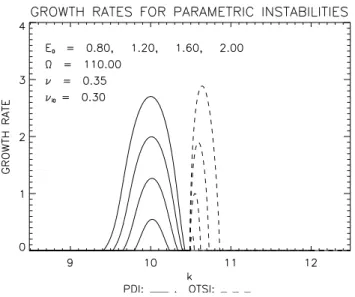
Fig. 1. Example of growth rates for the parametric instabilities. Solid lines for PDI and dashed lines for OTSI, for four values of E0,θ.
Eq. (10) to enter strongly in the Landau damping. For pa-rameter values where cavitation occurs, Landau damping is crucial. Therefore, wave numbers ranging up to the Lan-dau damping range kL ∼ 1/λD must be contained in the numerical model. On the other hand, the cascading steps have wave number decrements1k = 1/Xˆ. The numerical wave number space must resolve these intervals well. Con-sequently, the number of Fourier modesnx×nymust satisfy nx,y ≫2kL/1k∼3√M/(ηm)(the factor 2 arises, because both positive and negative must be included). This require-ment on the number of modes in most cases also ensures that the fairly narrow wave number ranges of the parametric insta-bilities are well resolved in the numerical model. The latter is very important; as an example, refer to Fig. 1: if the numer-ical wave number space does not hit near the maxima of the growth rates, the instabilities, as well as their mutual com-petition, might be misrepresented in the numerical model. Figure 1 will be further explained in Sect. 3.
rescaling the points on the broken line on Fig. 27 of Hanssen et al. (1992), with reduced mass ratio, will bring them into the cascading range. In this paper, efforts are made to re-tain parameters corresponding to realistic mass ratio, and the mode number is chosen accordingly.
The numerical method by which Eq. (6) is integrated is an integral part of the modelling. Periodic boundary conditions are used, implying that physics can go on in a system of fi-nite size, but still without boundaries. This makes our model a local model, where the background state is constant, spec-ified by the choice of values of the parameters of Table 1. The periodic boundary conditions then allow for optimized, two-dimensional fast Fourier transform routines to be used. Periodic boundary conditions are physically acceptable pro-vided the dimensions of the simulation cell are large com-pared to the intrinsic correlation lengths of the turbulence, as measured by the inverse width ink space of the dominant spectral features. For example, the size of the simulation cellL must be large enough that the resolution ink space 2π/L≪1k, where1kis the width of the cascade lines, as discussed above in the context of mode number requirement. The model described above is rich in dynamical behaviour, having a large parameter space, and no doubt, many aspects of the observed behaviour in the actual radio experiments is contained qualitatively in it. Even so, there is obviously im-portant physics left out of it. Among the major omissions and weaknesses we list the following:
1. The constraining to two space dimensions probably constitutes the most severe simplification. There are several aspects of this:
(a) For the cavitation range, the dimensionality is im-portant, both for the nucleation phase and the col-lapse phase. In 1D, nucleation is easy, while inertial collapse, wherein the cavitation asymptotically de-couples from the heater field, does not exist but di-rectly driven collapse is observed instead. Even so, numerical studies show that energy is transferred in k space to the Landau damping range also in this case (Hanssen et al., 1992; Hanssen, 1992). In 2D, numerics indicate that nucleation takes place less frequently, while inertial collapse now comes into existence. For 3D, numerical studies have been possible only with very poor wave vector space res-olution (Robinson et al., 1988). It is expected that the trend from 1D to 2D continues when passing from 2D to 3D. For example, collapse in 2D re-quires a threshold for the trapped energy, but not in 3D. Though, see our discussion of cases with largeB in Sect. 5, indicating that in the magne-tized case, things become more similar to 1D. (b) Constraining the excited dynamics to the magnetic
meridian plane, implies constraining out paramet-ric excitation by the component of the electparamet-ric field perpendicular to this plane. The latter is in
quadra-ture with the component in the magnetic meridian plane.
2. The reaction of the electron distribution function on the turbulence represents important physics left out of our present model. In the cavitation range, this is probably a very important feature: all particle simulations of HF generated Langmuir turbulence show that the electron distribution is perturbed by the Langmuir turbulence; thus, an energetic tail on the electron distribution will be formed. Recent reduced particle-in-cell simulations in Sanbonmatsu et al. (2000) indicate that for weakly driven systems, the fast particle acceleration has a neg-ligible effect on the turbulence levels and spectra. For more strongly driven cases, the turbulence levels are suppressed by increased Landau damping. One alterna-tive is to represent this by updating the electron distri-bution by a quasi-linear velocity space diffusion model, as has recently been done (Sanbonmatsu et al., 1999, 2000). On the other hand, this type of modelling is complicated by the intrinsic nonlocality of the problem; assuming that cavitation takes place in a thin layer in the vicinity of the O-mode reflection level, accelerated particles may leave this layer, but subsequently some of them may return after collision with heavy particles (Gurevich et al., 1985).
3. The locality of the model: the feature of accelerated electrons is already mentioned; here, we focus on other aspects of this. In the model (6), the background state is defined by a set of parameter values (cf. Table 1). However, these values are space dependent in the ex-perimental situation. This is in particular true for the electric fieldE0, the scale of which is given by the O-mode wavelength. Also, the spatial variation ofmay be important. The local model is justified if the meso-scopic variation of the background parameters, such as the density profile and the heater interference pattern, vary on scales large compared to the correlation lengths of the turbulence. In this case the predicted radar spec-trum can be represented as an incoherent sum of the lo-cally computed spectra over the observed altitudes. In the cascading range, different states will be coupled by Langmuir propagation, which is limited by Langmuir linear damping. In the cavitation regime, the spectra are broad, indicating small correlation lengths; here, the local approximation should be excellent. Accelerated electrons are also a potential mechanism of nonlocal coupling in all regimes. The recent resolved altitude or-dering of the observed turbulence (Rietveld et al., 2000; Cheung et al., 2001; Djuth et al., 2002) indicates that the local approximation is, in fact, valid, even in the cascading regime.
5. The inadequacy of the representation of the kinetic de-scription of the ion dynamics has been mentioned above and is discussed by Stubbe et al. (1992b) and DuBois et al. (1995). A 1D numerical study with linearized Vlasov dynamics of the ions has been presented by Helmersen and Mjølhus (1994); it showed the same qualitative features as obtained in the 1D Zakharov model, al-though a bias towards the cavitation regime was found. Vlasov simulations (Wang et al., 1994, 1995) and re-duced particle-in-cell simulations (Sanbonmatsu et al., 1999, 2000) with particle electrons and ions have shown the same qualitative features as predicted by the Za-kharov model and in some weakly driven cases, quan-titative agreement between the models was obtained as mentioned above.
The driven and damped character of the model (6) should be emphasized, as opposed to the conservative version (Za-kharov, 1972) often emphasized in earlier work. The drive represented byE0is clearly exhibited when the energy bal-ance equation for the model is written up. Using the proce-dure on p. 17 530 of Mjølhus et al. (1995), the balance
d
dtU¯ = ¯W− ¯D (12)
can be obtained, where
¯ U= 1
2
Z
T2|∇
9|2dx (13)
is the electrostatic energy in the simulation cellT2,
¯ D= 1
2
Z
T2
∇9·(νe∗ ∇9∗)+c.c.dx (14) the dissipation, and
¯ W =1
2iE ∗ 0·
Z
T2
n∇9dx+c.c. (15)
is the Joulean energy injection into the cell (Doolen et al., 1985). The energy loss from the incident radio wave is a global effect that is not represented in the local model (6); instead, a spatial damping on a global scale can be accounted for (Mjølhus et al., 1995).
3 The dispersion relation
The feature of external drive, represented by the complex vectorE0, implies that the unperturbed staten=0,∇9 =0 may be unstable, typically when|E0|is above some thresh-old. The instabilities, the parametric decay instability (PDI), and the “Oscillating Two-Stream Instability” (OTSI), are well-known. However, the dispersion relation leading to these instabilities from the model (6) is quite complex, and so we discuss here some useful approximate formulas and general features.
In particular, it is intended to exhibit explicitly the depen-dence of the modes on the geometric features. Fortunately,
the basic formulation of this aspect is rather simple: stabil-ity is investigated by considering plane wave solutions of the linearization of Eqs. (6); however, plane wave implies 1D spatial variation, so one will come to the same result by con-sidering the constraining of Eqs. (6) to dependence on one spatial direction, and thereafter, linearize and Fourier ana-lyze. A unit vector in this direction is denoted byeξ, and the spatial coordinate in that direction is denoted byξ. Then, the system of Eqs. (6) is readily brought into the form
h
i(∂t+ν∗)+(θ−n)+∂ξ2
i
E=E0,θn−ij2 (16a) (∂t2+2νi∗∂t−∂ξ2)n=∂ξ2|E+E0,θ|2 (16b) after one integration of Eq. (6a). Here, E = ∂ξ9, j2 =
−ihnEi(spatial average) can be considered as a constant of integration (for example, necessary to make9 well-defined on our periodic numerical model), and
E0,θ =E0·eξ (17a)
θ =−Bsin2θ , (17b)
where θ is the angle between the direction eξ and the ex-ternal magnetic field. It is seen that Eq. (16) has the form of a 1D Zakharov system, such as, for example, considered in Hanssen et al. (1992); the geometric features enter only through the parametersE0,θ andθ of Eq. (17). In partic-ular,E0,θ can now be considered real and positive, with no loss of generality, because any phase can be absorbed intoE. For the case ofE0real (i.e. the two components in phase), one has
E0,θ =E0cos(α−θ ) , (18)
whereαis the angle betweenE0and the magnetic field di-rection. Linearizing Eq. (16) around the vanishing state and subsequently Fourier analyzing as∼ exp[i(kθξ −ωt )], the quartic dispersion relation
P0(ω)=2kθ2µE02,θ (19)
with P0(ω)=
4
Y
j=1
(ω−ω0j) , (20)
where ω01=µ−iν
ω02= −µ−iν
ω03=ckθ−iνi0|kθ|
ω04= −ckθ−iνi0|kθ|
c=
q
1−νi20 µ=kθ2−θ
represented independently by complex amplitudes. Alterna-tively, one can treat E andE∗ (complex conjugate) as in-dependent. E∗is then often referred to as the “anti Stokes component”.
In Eq. (19), we considerωas unknown, andk,θ,E0,θ, νandνi0as parameters. In general, the 4 roots of Eq. (19) have a complicated dependence on these parameters. In the limitE0,θ = 0, we have the roots ω = ω0j,j = 1, ...,4, which represent the Langmuir wave described byE (ω01), the Langmuir wave described byE∗(ω02), and the forwards and backwards propagating sound wave (ω03andω04). The Langmuir mode propagates forwards (backwards) whenk > 0 (<0).
Instabilities, i.e. positive values of the imaginary part of the roots of Eqs. (19) and (20), exist near values ofk for which the real parts ofω0j coalesce. The PDI, with right-moving Langmuir wave and left-right-moving ion-acoustic wave, occurs when Re(ω01)=Re(ω04), e.g.k2θ −θ+ckθ =0, kθ >0, also implying Re(ω02)=Re(ω03), which gives
ˆ
kθ = −c 2 +
q
θ+c2/4. (21)
Similarly, for the left-moving Langmuir wave (kˆθ < 0) and the right-moving ion-acoustic wave, the resonance condition is Re(ω01)= Re(ω03), leading to the negative of Eq. (21). For these two situations,µ < 0, implying a negative fre-quency shift, a well-known property of parametric instabili-ties of decay type.
The OTSI occurs near values ofk, for whichω01 andω02 are both zero, i.e.µ=0. At the exact valueµ=0, the cou-pling term (i.e. the right-hand side of Eq. (19)) again van-ishes, so for that value of k the roots are the modes ω0j, which are all damped. As it turns out, this instability ex-ists for a range of values ofkθ for whichµ >0. In Fig. 1, an example of the growth rates of each of them as a function of kat increasing values ofE0,θ are plotted, as computed from Eq. (20). The growth ranges, i.e. the range ofkwith positive growth rate, are seen to be relatively narrow. More useful: the pointµ=0 cannot be in any of the growth ranges for the reason stated above; therefore, this condition separates the growth ranges of the two instabilities. This is a useful cri-terion to identify the two instabilities when solving Eq. (19) numerically.
From Fig. 1, the competition between the two instabilities is also seen; the OTSI has the largest threshold, but its growth rate increases more rapidly withE0,θ, so that it wins at higher values, at least at sufficiently small values ofθ.
In order to obtain useful formulas for the two instabili-ties, a natural approximation is to substitute the resonance condition into the two non-resonant factors on the left-hand side of Eq. (19); this will give quadratic equations for the growth rates. Consider first the PDI. Assuming the resonance condition, implying Eq. (21), putω = µ = −ckˆθ and ne-glect damping in the two nonconfluent factors of (19), and ω=µ+iγ = −ckˆθ+iγ in the confluent factors; this gives γ2+ν+νi0| ˆkθ|
γ −
1
2kˆθ E0,θ
c −ννi0| ˆkθ|
=0. (22)
Fig. 2. Example of maximum growth rates for the PDI instability as a function ofθ for three different values ofE0,θ. Dashed lines show result from using two-mode formula.
ForE0,θ> E0,t, where
E20,t =2cννi0, (23)
Eq. (22) has one positive (and one negative) real root; thus, E0,t is the threshold value in approximation (22). This threshold is not an exact result from Eq. (19), although it is a very good approximation in most situations. The true threshold increases somewhat whenθ decreases. ForE0,θ above this threshold, the maximum growth rate according to Eq. (22) is
γM,P DI = − 1 2νi0| ˆkθ|
+
s
1 2
ˆ
kθ(E02,θ−E02,t)
c +
1 4ν
2
i0| ˆkθ|2, (24) where ν ≪ νi0|k|was assumed. Just above the threshold, the second term under the square root will dominate, and one has the simplified formula
γM,P DI ≃ 1 2
(E02,θ−E02,t)
cνi0
. (25)
In the opposite limit: far above threshold, one has the simpli-fied formula
γM,P DI ≃ 1 2kˆθ
E02,θ
c
!1/2
−1
2νi0| ˆkθ|. (26) A closer inspection shows that the two-mode approxima-tion (22) requiresE02,θ/kˆθ ≪1. In Fig. 2, we show the PDI growth rate as a function ofθ, for 3 values ofE0,θ, and compare it with the two-mode formula (24).
Fig. 3.Example of maximum growth rates for the OTSI instability as a function ofθfor three different values ofE0,θ. Dashed lines show result from using two-mode formula.
numerical study showed that this is an excellent approxima-tion, although apparently neither is fully exact.
For the OTSI instability, one can analyze Eq. (19) as fol-lows: first, substitutingω =iγ, the left-hand side becomes a polynomial with real-valued coefficients. Next, a condition for the constant term to vanish is
ν2+µ2−2µE02,θ=0. (27)
At values ofkwhere this is satisfied, the dispersion relation has a rootγ =0. Assuming this is a simple rootγ (k)which has∂kγ 6=0, there will be values ofkin the neighbourhood for whichγ (k)is positive (as well as negative). Thus, there is a purely growing instability. Actually, Eq. (27) defines two values ofkwhenE0,θ > E0,t, where
E02,t =ν (28)
and there is positive growth rate precisely between these val-ues. Equation (27) clearly shows thatµ >0 for this to hap-pen. The threshold (28) is exact (within the model (6)). In or-der to obtain simple approximate expressions for the growth rate, we neglect again the growth rate in the acoustic factors of Eq. (19), while retaining it in the two confluent factors, giving
(γ +ν)2+µ2−2µE02,θ =0. (29) It is readily seen that the largest growth rate occurs forµ= E02,θ, e.g.kθ =(θ+E20,θ)1/2. This gives
γM,OT SI = −ν+E02,θ. (30)
In Fig. 3, the numerically computed maximum growth rate of OTSI is plotted as a function ofθ, together with the results using formula (30), for three different values ofE0,θ. It is seen that Eq. (30) is not a particularly good approximation
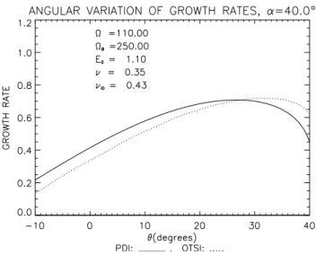
Fig. 4. Example of maximum growth rates for the OTSI and PDI instability as a function ofθforα= 40 andνi0= 0.45. Dashed line shows OTSI growth rate and solid line shows PDI growth rate.
at higher values of E0,θ. By comparing Figs. 2 and 3, or considering Fig. 1, it can be seen that, at the smaller values ofθ and larger values ofE0,θ, the OTSI may have a larger growth rate than the PDI, with respect to a fixed direction. In Hanssen et al. (1992), it was concluded from numerical material that the dynamics goes to cavitation when the OTSI has the largest growth rate. An original motivation for the present study was to look for this to happen when the drive is off-parallel. For example,α may be small andE0,α large, so that the OTSI has the largest growth rate in directionα. However, looking at directionθwithα > θ > 0, one sees from Eqs. (17) thatθincreases while going towards smaller θ, whileE0,θwill decrease. This trade-off may result in PDI having the largest growth rate, occurring at an angleθm,α > θm > 0. In Fig. 4, we show a case where the OTSI has (slightly) the largest overall growth rate. It does not seem worthwhile to express this trade-off analytically.
The angular growth range of the PDI, defined as the range of directionsθfor which the PDI has a positive growth rate, can be obtained from Eqs. (23) and (18) as
α−θc< θ < α+θc, (31)
where cosθc=
√
2ννi0c
E0 . (32)
4 Observability: geometric aspects
Radiated Power (ERP), 3–9 MHz) transmitter located 17 km to the northeast of the radar. The EISCAT facilities consist of a high power (<1.2 GW ERP) HF transmitter located near Tromsø, Norway, which can operate in the frequency range 3.85–8.0 MHz, and two diagnostic radars of 224 MHz (VHF) and 933 MHz (UHF). The UHF radar, in addition, has remote receivers in Kiruna, Sweden, and Sodankyl¨a, Finland.
The radar predictions from the model (6) are made as fol-lows:
1. Using a spectral method for generating a numerical so-lution to Eq. (6), it will consist of nx ×ny time se-ries9(t;k),n(t;k), where nx (ny) are the number of Fourier modes inx (y) directions (wherek =(kx, ky) takesnx×nyvalues).
2. Each radar configuration described above defines a cer-tain wave vectorkpfor Bragg scatter as
kp= ±2k0cos φ
2 eφ/2 (33a)
k0=ωR/c , (33b)
whereωR is the (angular) frequency of the radar,φis the angle between the lines of sight of the transmitting and receiving radar to the ionospheric volume element being probed, andeφ/2a unit vector bisecting the angle between these lines.
3. One can then select the complex time series9(t; ˜kp), n(t; ˜kp), wherek˜p is the (discrete) wave vector in the numerical model that best approximateskp, and per-form a discrete Fourier transper-form overmselected time subintervals of equal length, and form the averaged power spectra
Sp(ω)= 1 m
m
X
j=1
| ˜k2p9j(ω; ˜kp)|2 (34a)
Si(ω)= 1 m
m
X
j=1
|nj(ω; ˜kp)|2. (34b)
Here, the indicesp,istand for “plasma line” and “ion spectrum”, respectively. For the three radars, we are us-ing the valueskp = 9.38 m−1(EISCAT VHF), kp = 18.01 m−1 (Arecibo), andkp = 39.08 m−1 (EISCAT UHF, monostatic mode). In Sect. 5, we refer to dimen-sionless quantities; thenkp 7→ ¯kp = ˆXkp, whereXˆ is given in Eqs. (7).
Thus, our model is that these spectra are proportional to the contribution to the observed radar spectrum arriving from the particular ionospheric location modelled by the param-eter values entered into Eqs. (6), in the “plasma line” and “ion line” bands, respectively, (DuBois et al., 1988, 1990; Hanssen et al., 1992). We shall refer to these power spec-tra at fixed wave vectors as “virtual radars”. The ability to
extract plasma line and ion line power spectra from the sim-ulation data is perhaps the most important diagnostic in the recent approach to Langmuir turbulence and led directly to predictions of cavitating turbulence features near reflection density (DuBois et al., 1988), which were subsequently iden-tified in experiments (Cheung et al., 1989). We note that no other approach to this problem has produced power spectra.
The theoretical prediction of observability of the HF-generated Langmuir turbulence is then related to the occur-rence and strength of a Fourier component atk˜pin the gen-erated solution. This, in turn, depends on the parameters de-scribed in Sect. 2. In particular, the direction and strength of
E0is decisive. Of particular interest is the polarization and electric field amplitude at the matching stateX = Xmatch, where waves of frequencyω0and wave vectorkpsatisfy the Langmuir dispersion relation
1−Xmatch=3(λDkp)2+Y2sin280, (35) where80is the angle between the radar line of sight and the magnetic field direction, andX=ωpe2 /ω20is the normalized plasma frequency. In the dimensionless quantities of Sect. 2, this takes the form
¯
k2p+ ¯kp=φ0 , (36)
whereθis defined in Eq. (17b) (the second term on the left-hand side of Eq. (36) is not included in Eq. (35); it represents the frequency downshift of the decay instability).
In order to describe the aspects of electric field polariza-tion and amplitude in more detail, it was natural to referE0to two different orthonormal right-hand bases (see Fig. 5). For a description of polarization, the baseek,e⊥,ezis used, where ekis along the magnetic field direction,e⊥is perpendicular toek, but in the magnetic meridian plane, andezis perpendic-ular to the magnetic meridian plane. For a description of the energy conservation and ray optics in a horizontally plane-stratified medium, X = X(ξ ), the baseeξ,eη,eζ is more natural, whereeξ points vertically,eη points horizontally in the magnetic meridian plane, andeζ =ez. The components ofE0are then connected as
E0,ξ =E0,kcosα0+E0,⊥sinα0 (37a) E0,η= −E0,ksinα0+E0,⊥cosα0 (37b)
E0,ζ =E0,z, (37c)
whereα0is the angle between the vertical and the magnetic field.
The polarization relations can now be taken from Stix (1962), and read
E0,⊥= −RE0,k (38a)
E0,z=iσ E0,⊥ (38b)
where
R= 1−X−N 2sin2θ
N2sinθcosθ (39a)
σ = D
Fig. 5.Coordinate unit vectors. (a) The meaning ofθ. (b) Coordi-nate vectors oriented with respect to vertical vs. those oriented with respect to the magnetic field.
andǫ⊥=1−X/(1−Y2),D=XY /(1−Y2). The O-mode index of refractionN is given by
N2=1− X(1−X)
1−X−12Y2sin2θ+1 (40a) 1=
"
(Y (1−X)cosθ )2+
1 2Y
2sin2θ
2#1/2
. (40b)
Here,θhas the same meaning as in Sect. 3, namely the angle between the currentk and the magnetic field. For normal (i.e. vertical) incidence and plane-stratified medium,θ =α0, otherwiseθwill vary along the ray path, and will have to be determined by ray tracing.
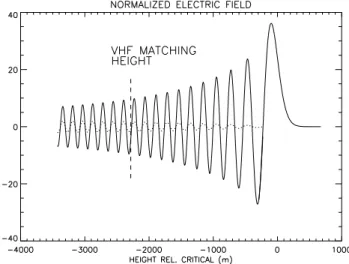
Fig. 6.Example of the spatial structure of the electric field of a nor-mally incident radio wave just below the critical height, according to (46) and (48) (withEˆ0=1). Solid line:E0,k, broken line:E0,⊥. The parameters: ω0 = 2πf0 withf0 = 4.544 MHz, α0 = 12◦, Y = fce/f0withfce = 1.35 MHz, andL = 160 km. The VHF matching height is marked according toTe=0.17 eV.
The most commonly used model to estimate the strength ofE0 at a given location, e.g. the matching height, has the following two steps:
1. Often, the transmitter power is given as ERP (Equiva-lent Radiated Power). Then, at vertical heightH and angle of incidenceθ0(relative to the vertical), the verti-cal component of the time-averaged Poynting flux is
¯ Pξ =
Qcos3θ 0
4π H2 , (41)
where, for simplicity, straight rays are assumed. 2. For propagation over distances much smaller thanH, in
the vicinity of the O-mode reflection levelX = 1, the following model is usually adapted:
(a) plane-stratified medium,X=X(ξ ), and
(b) parallel rays, kη = ωcNη = const., whereNη is related to the angle of incidence byNη=sinθ0. Then, the variation of the wave amplitude is governed by the conservation ofP¯ξ, which is given by
¯ Pξ =
c 8π
Nξ(|E0,ζ|2+ |E0,η|2)
−Nη1 2(E0,ηE
∗
0,ξ+c.c)
, (42)
where Nη,ξ = (c/ω)kη,ξ are the dimensionless wave vec-tor components. Using the polarization relation (38) and the transformation (37), the components of the electric field am-plitude can be expressed as
E0,k=KkEˆ0 (43a)
whereEˆ0is a reference electric field amplitude determined as theηcomponent of a vacuum circularly polarized wave electric field at heightH and angle of incidenceθ0, which from Eqs. (41), (42) is given by
ˆ
E0= Qcos 4θ
0 cH2
!1/2
. (44)
(WhenQis given in watts, we obtainEˆ0in SI units volts/m by substituting 1/c7→cµ0/4π, whereµ0=4π×10−7.) In Eq. (43), the swelling factors are given by
Kk=
2
cosθ0
1/2
K0 (45a)
K⊥= −RKk (45b)
K0=
n
Nξ
h
σ2R2+(sinα0+Rcosα0)2
i
+Nη(sinα0+Rcosα0)(cosα0−Rsinα0)
o−1/2
. (45c) In the case of vertically incident wave,θ0=0, e.g.θ =α0, the incident and reflected wave will overlap, and the spatial structure of the electric field should be described as
Ek(ξ ) E⊥(ξ )
=2
Kk K⊥
ˆ E0sin
Z 0
ξ ω0
c N dξ+ π
4
!
, (46)
whereKkof (45) in this case is given by
Kk=
2
N[σ2R2+(sinα0+Rcosα0)2]
1/2
, (47)
Nis given by (40), andξ =0 atX=1. Equations (46), (47) break down asξ → 0 (X → 1), becauseN → 0 in (47); then just belowX=1, (46), (47) overlap with
E0,k=2
√
2πω0 c L
1/6
sinα0−2/3Eˆ0Ai(ξ / l) (48a)
E0,⊥=0, (48b)
whereLis the scale height defined as dX/dz|X=1 = 1/L, Ai(v)is the Airy function of argumentv(Abramowitz and Stegun, 1970), andl =(c2Lsin2α0/ω20)1/3. Equation (48) is based on an approximationN2≃(1−X)/sin2α0, valid in the immediate neighbourhood ofX=1. A computed exam-ple is shown in Fig. 6, based on parameters of the experiment of Rietveld et al. (2000). From Eq. (48),
maxE0,k=KAiEˆ0, (49)
where the swelling factor for Airy maximum is given as KAi =2√2πω
cL
1/6
sinα0−2/3max Ai, (50) where the maximum value of the Airy function is max Ai= 0.536 attained at ξ / l = −1.0 (Abramowitz and Stegun, 1970). This gives the value
Ai = 3 4η
M m
ω
0 c
L sinα0
−2/3
(51)
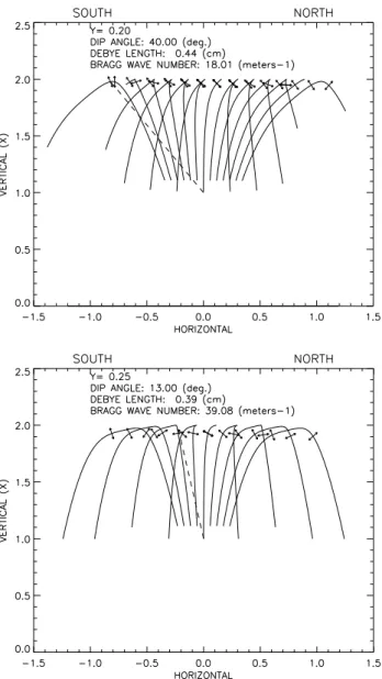
Fig. 7.Some examples of rays above HF transmitter, with polariza-tion (ofE0component in the magnetic meridian plane) at match-ing height indicated by arrows. The ray tracmatch-ing model underly-ing this, as well as Figs. 8 and 10, is briefly sketched in the main text, where the horizontal and vertical length scales are also ex-plained. (a)A case corresponding to the Arecibo setup: dip angle 40◦, Y = 0.2, based onfce = 1.05 MHz, Bragg wave number 18.01 m−1, Te = 0.12 eV (for calculation of matching height).
(b)A case corresponding to the EISCAT UHF setup: Y = 0.25 (based onfce = 1.35 MHz), dip angle 12◦, Bragg wave number 39.08 m−1,Te=0.1 eV.
for at Airy maximum. At the end of this section, Airy swelling at oblique incidence is briefly discussed. Alterna-tively, the uniform approximation of Lundborg and Thid´e (1986) could have been used.
ˆ
E0 = 0.346 V/m, which gives E0,k = 3.3 V/m at match-ing height and E0,k = 13.2 V/m at Airy maximum. For the parameters of Fig. 6, we have Ecˆ = 0.94 V/m, giv-ing dimensionless valuesE0,k =3.5 (matching height) and E0,k = 14.0 (Airy maximum). These are rather extreme values, compared to those that have been used in numer-ical solutions of the model (6) or its one-dimensional ver-sion. Extreme values were also noted by Lundborg and Thid´e (1986) (cf. p. 493), and Djuth et al. (2002). For compari-son, applying the same model to an Arecibo case (α0=40◦, fce = 1.05 MHz,f0 = 5 MHz, L = 50 km, Q= 80 MW (ERP),H = 245 km, Te = 0.12 eV),E0,k = 1.3 V/m at matching height (dimensionless: 1.5) andE0,k = 3.0 V/m (dimensionless: 3.5) at Airy maximum were obtained. Al-though far more moderate, still these values are large com-pared to those that have been used previously in theoretical work based on the model (6).
For the case of oblique incidence, the direction of the wave vector, i.e. the angleθ, must be determined by solving the Booker quartic (Budden, 1985) forNξ. We have developed a ray tracing model by simply considering the Booker quar-tic as a Hamiltonian and thus, following its O-mode root. Some results of this have been shown in Figs. 7 and 8. In our simplified model, we assume a vacuum up to 100 km, then a linear density profile withL=100 km up to the critical level X =1, thus, interpreting the units on the axes of Figs. 7, 8, and 10 as 100 km.
In Fig. 7a, we show 13 rays, ranging from angles of in-cidence 18◦to the south to 18◦to the north, for a case cor-responding to the Arecibo setup. The magnetic field direc-tion is shown by means of a dashed line. The polarizadirec-tion at matching density is shown by means of arrows. For the central vertically incident ray, the polarization is seen to be essentially parallel to the magnetic field, thus, making an an-gle of∼ 40◦with the line of sight. On the other hand, for the southernmost rays, it is seen that the polarization in the downleg is more favourable. Figure 7b shows a similar pic-ture for the Tromsø UHF case (9 rays with incidence from 12◦ south to 12◦ north). For the central ray (vertical inci-dence), one sees that the polarization at matching height is indeed very unfavourable. Again, the most favourable cases are the downward moving rays to the south. In Kohl et al. (1987) it is stated that, by experience, a “useful” configu-ration for plasma line observation with EISCAT UHF is to tilt the heater beam 6◦ to the south and observe along the magnetic field. We shall refer to this as the “Kohl setup”. This corresponds approximately to the second ray towards the south counted from the central (vertical incident) ray. For the central, vertically incident ray, the polarization at VHF matching height is nearly along the magnetic field. Usually, in Heating-EISCAT VHF experiments, both the Heater and the VHF antenna are oriented vertically.
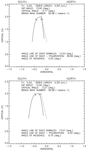
Let us elaborate a little further on the configuration based on the downward moving wave in the EISCAT UHF case. In Fig. 8a, b we show single rays at vertical incidence, 5.5◦ (a) or 6.75◦(b) to the south. It is seen that the rays make a
Fig. 8. Single rays to further illustrate the dependence of the po-larization of the pump field at EISCAT UHF matching height on plasma parameters.(a)Y =0.25; Debye lengthλD=0.5 cm (cor-responding to applied frequencyf0=5.4 MHz andTe=0.16 eV).
(b)Y = 0.2; λD = 0.3 cm (corresponding to applied frequency f0=6.75 MHz andTe=0.09 eV).
coun-Fig. 9.Solid line:Kk, broken line:K⊥, at EISCAT UHF matching height on downleg, as a function of the applied frequency.
teracts this effect. In Fig. 9, this effect is illustrated quantita-tively.
It is tempting to refer to the experimental work of West-man et al. (1995) in this connection: by changing the ap-plied frequency from 5.423 MHz to 6.77 MHz, a plasma line spectrum was obtained with the monostatic UHF configura-tion with unprecedented detail: decay line and 5 cascades could be counted. The configuration corresponds by far to the one modelled in Fig. 8a: λD = 3 mm,Y = 0.2 which withfce=1.35 MHz corresponds tof0=6.75 MHz; more-over, the angle of incidence of 6◦ and direction of sight of 12◦also corresponds to the experiment.
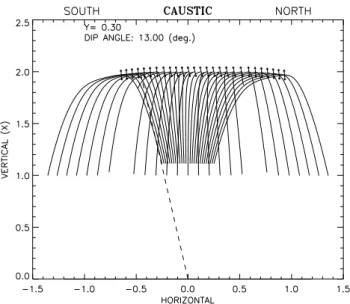
Fig. 10.The caustic of the ray bundle for Tromsø parameters. The arrows show the polarization of the electric field component in the magnetic meridian plane at the turning point.
Fig. 11. The mismatch parameterat the turning point as a func-tion of the angle between the direcfunc-tion of the line of sight towards the turning point and the vertical. The markers indicate the spitze.
It is well-known that the Tromsø UHF plasma line is dif-ficult to observe in the range of larger Debye lengths, e.g. high temperature and low applied frequency. This has usu-ally been attributed to an increased Landau damping, which increases the threshold (Stubbe et al., 1985). The feature il-lustrated in Fig. 8a, b offers an alternative explanation to this observation.
We have compared the Landau and collisional damping rates in the actual parameter range. Details are omitted. We concluded, as did Stubbe et al. (1985), that the Landau damp-ing explanation is also feasible. The polarization feature de-scribed above represents an added effect.
Recently, there has been a de-emphasis of the role of the matching height for these oblique HF-UHF experiments and an increased emphasis on explanations in terms of cavitation (Isham et al., 1999b). For the Kohl setup (with the UHF radar pointing along the magnetic field), the HF wave field will not reach the critical levelX =1 on the radar line of sight, ac-cording to our horizontally stratified model. We shall call the highest point of a given ray (specified by its angle of in-cidenceNη =sinθ0and the plasma parameters) its turning point; other names may also exist. Thus, it has become of interest to discuss the possibility of explaining UHF observa-tions as due to cavitating Langmuir turbulence near the turn-ing point at oblique incidence. In the followturn-ing, we report briefly on a study of what the input parameters to model (6) will be near the turning point, in particular, as seen at the line of sight 13◦south.
Fig. 12. The swelling factor as a function of angle of incidence, relative to that of normal incidence (as given by Eq. (50)). The broken line indicates(sinα0)2/3withα0=13◦, corresponding to the unmagnetized case.
mismatch parameterat the turning point, as a function of the angle between the vertical and the line of sight. It is seen that the value ofat the turning point seen at 13◦south in the chosen example is around 100, i.e. as a rule-of-thumb, comparable with the value at VHF matching height.
Near the turning point, there will also be a swelling of the electric field amplitude, as in the case of vertical incidence described above. It should be stated that the relevant concept here is the caustic rather than the turning point, where the caustic is the envelope of the rays. We choose to replace the caustic by the turning point, which we expect to be a good approximation. The turning point will be the caustic for par-allel rays, i.e. fixedNηfor all rays. Then the electric field in the vicinity of the turning point will be described by an Airy function of the vertical coordinate, in addition to the polar-ization relations at the turning point. The appropriate theo-retical formulation of this for the case of oblique incidence does not exist in published form, according to the authors’ present knowledge. In particular, at normal incidence, the factor sinα−2/3occurs in the swelling factor, which gives a strong extra swelling effect at high-latitudes. It is of interest to find out how this swelling effect behaves at oblique inci-dence. In Fig. 12, we show the swelling factor relative to that given by Eq. (50), as a function of angle of incidence. At the two critical directions, it formally goes to 0, however, near those values, the calculation is not valid anyway be-cause coupling to the Z-mode takes place (Mjølhus, 1990). It is seen that for incidence around 10◦, the swelling factor is still around half that of normal incidence. The details on the computations leading to Fig. 12 will be described elsewhere. It is emphasized that the simple model described above should be considered as a reference model only. The two main sources of deviation are:
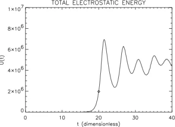
Fig. 13. Time evolution ofU(Eq. (52)) for example I. Onset of averaging marked.
1. absorption,
2. refraction due to large-scale irregularities introducing horizontal gradients.
Both of them are essentially uncontrolled and unpredictable and it would, therefore, scarcely be of any help to try to im-plement them into the model. On the other hand, the electric field distribution in actual experiments must be expected to be influenced by these factors. For the absorption, there are two main components:
1. Absorption in the lower ionosphere (D layer), where the neutral density and consequently the collision frequency is high. This depends very strongly on the actual degree of ionization of these lower layers. It is also a question to what extent this ionization can be influenced by the high-power HF wave.
2. Anomalous absorption of the HF wave near the critical layer due to the energy loss into generation of the Lang-muir turbulence, along the already traversed part of the ray path. For long duration high duty cycle exposure, one will also have strong anomalous absorption due to striations (e.g. Jones et al., 1984).
5 Some numerical examples
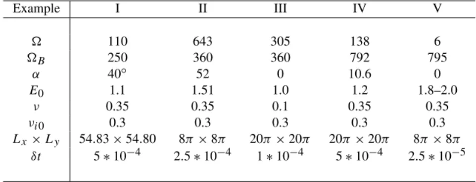
In this section, we show some selected examples of results of numerical solutions to Eqs. (6), in order to illustrate fea-tures discussed in Sects. 3 and 4, as well as to shed some theoretical light on recent experiments. The parameters of the examples are listed in Table 2.
Table 2.
Example I II III IV V
110 643 305 138 6
B 250 360 360 792 795
α 40◦ 52 0 10.6 0
E0 1.1 1.51 1.0 1.2 1.8–2.0
ν 0.35 0.35 0.1 0.35 0.35
νi0 0.3 0.3 0.3 0.3 0.3
Lx×Ly 54.83×54.80 8π×8π 20π×20π 20π×20π 8π×8π δt 5∗10−4 2.5∗10−4 1∗10−4 5∗10−4 2.5∗10−5
channel the valueω = 0 corresponds to no frequency shift relative to the applied frequencyω0, and positive (negative) values ofωcorrespond to outshift (inshift). The frequency resolution isδω = 2π/(N1δt ), whereN1 is the number of sampled values andδtis the time step.
Example I (Figs. 13–14) is intended to illustrate the ge-ometric aspects of the maximum growth rates of the para-metric instabilities, as discussed in Sect. 3 and illustrated in Fig. 4. In fact, the parameters of example I are the same as those of Fig. 4. In Fig. 13, we show the overall evolution by exhibiting the time evolution of the quadratic sum of all the
Fig. 14.Contour plots of time-averaged modal spectra, example I. Direction of driving electric field indicated with arrow in upper panel.
Fourier modes U (t )=
ny
X
jx=1 nx
X
jy=1
|k9(kjx, kjy, t )|
2, (52)
which is proportional to the total electrostatic energy of the simulation cell. One can see a growth stage, 0≤t ≤20 (in units (7)), and thereafter, in this case, damped modulations. In Fig. 14, we show contour plots of the time-averaged modal spectra,h|k9(k, t )|2i,h|n(k, t )|2i, where the averaging goes overtave ≤ t ≤ tend, withtave = 20 and tend = 40 in this case. In the upper panel, the direction of the driving electric field is indicated by an arrow (α = 40◦in this case). The primary decay and two cascades can be seen. The excita-tion maximum in thek-plane is not along the driving electric field, but it agrees reasonably with the direction of maximum PDI growth rate of Fig. 4 (max excitation occurs in the range 20◦< θ <25◦, while the theoretical max growth rate occurs atθ =27◦).
In the spectrum ofn(lower panel), the primary decay (A) and the two first cascades (B) can also be seen; in addition, there is a spectrum in a range neark=0(C) corresponding to density channels along the group velocity of the primary decay.
A feature of example I is that the OTSI has the overall largest growth rate. In addition, the system sizesLxandLy were chosen such that thekof maximum growth rate of the OTSI was approximated optimally in the numerical system. Still, the outcome of example I is saturation by cascade.
as-Fig. 15.Same as Figure 14, but for example II.
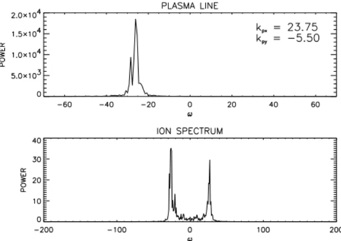
suming a scale heightL = 35 km. We have calculated the polarization at the matching height to make an angle of 52◦ to the magnetic field. We chose a fairly largeE0 (= 1.51), corresponding to the “super heater” (1.2 GW ERP) used by Djuth et al. (1994). With gyrofrequencyfce = 1.35 MHz, η=2.5 and mass ratioM/m=3∗104, we haveB=360. Some results of example II are shown in Figs. 15–17. Fig-ure 15 shows the modal spectra, averaged over 15≤t ≤40. In the upper panel, the electric field polarization and the vir-tual radar are indicated. One sees that this example again appears as cascade-saturated. Figure 16 shows sections of the modal spectrum ofEalong the two directions indicated in Fig. 15. The wave number of primary decay instability in the two directions, according to Eq. (21), are indicated. We see that along the radar direction, the maximum excitation is not at the primary decay. The excitation level along the radar direction is∼1/30 of that along the driver direction.
Figure 17 shows the virtual radar spectra for this situa-tion. It will be interesting to compare them with virtual radar spectra of example V. In example II, we ran 9 nearby virtual radars. Surprisingly, the frequency downshift of the plasma line varied considerably in the range−10> ω >−40.
Also, the setup at Arecibo has been recognized as geomet-rically unfavourable, with the E0polarization nearly along the magnetic field, and the radar line-of-sight usually along the vertical, making 40◦–45◦ withE0, cf. Fig. 7a. This is discussed in detail in DuBois et al. (2001) and Cheung et al. (2001). In example III, we show a case pertaining to that
Fig. 16. Sections of the modal spectrum ofEalong the direction ofE0(upper) and along the radar probing direction (lower), exam-ple II. Locus of primary decay indicated by vertical dotted lines.
Fig. 17.Virtual radar spectra for example II. Five half-overlapping subspectra of lengthN1=215, sampled with time stepδt =2.5∗ 10−4.
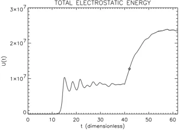
Fig. 18. Time evolution ofUfor example III. For 0≤ t ≤40, it was run withν=0.25, while for 40≤t ≤62,ν =0.1. Onset of averaging and virtual radar sampling att=42 marked.
Fig. 19. Contour plots of time-averaged modal spectra for exam-ple III. Driver and virtual radar indicated in upper panel.
for the electron collision frequency, DuBois et al. state that νec/ωpe=1.5∗10−5. From this we obtainν=0.1. Finally, DuBois et al. putνi0 = 0.32445 (again, “best fit two-pole approximation”).
The results for example III are shown in Figs. 18–20. The plasma line strength of Fig. 20 is about half that of Fig. 22 below, while the ion spectrum is about one-fifth of the latter.
Fig. 20. Virtual radar spectra for example III. Three half-overlapping subspectra of lengthN1=214, sampled with time step δt=10−4.
It is also interesting to compare with the results of Mjølhus et al. (2001), where radar matching of numerically generated Langmuir spectra was promoted by refraction in plasma den-sity ducts. Both virtual radar spectra of Fig. 8 of Mjølhus et al. (2001) are about one-half of the corresponding spectra of Fig. 20.
As has been emphasized in many papers, the main pre-diction from the model (6) is saturation by decay-cascades at some distance below the O-mode reflection level, which will be observable by a radar detecting scattered signal from the radar’s matching height Eq. (34), and a cavitating turbu-lence just below the reflection level, expected to be observ-able by a range of radars (Hanssen et al., 1992; DuBois et al., 1993a, b; 2001). This qualitative prediction has indeed been supported by experiments in great detail (Sulzer and Fejer, 1994; Rietveld et al., 2000; Cheung et al., 2001; Djuth et al., 2002). In particular, Rietveld et al. (2000) presented an ex-ample with height-separated spectra of cascade versus cavi-tation type obtained by the Tromsø VHF radar. In Sect. 4, we made estimates of the electric field strength and polarization for data corresponding to that experiment. In the next two ex-amples, we show numerical results obtained for parameters chosen relative to the Rietveld et al. (2000) experiment.
Let us first emphasize that, by using electric field values as estimated in Sect. 4, or corrected for, say, 30% D-layer absorption, (i) model (6) cannot currently be handled numer-ically, and (ii) would be expected to lead to a prediction of cavitating Langmuir turbulence in all of the height ranges from which HF-enhanced backscatter was obtained by the EISCAT VHF radar in the Rietveld et al. (2000) experiment. In the examples we show, we have used far smaller values of E0than those estimated in Sect. 4.
correspond-Fig. 21.Contour plots of modal spectra, example IV. Averaging and virtual radar sampling were done for 60≤t ≤ 90. Virtual radars (3) and driver indicated in upper panel.
ing to vertical probing. The component of the driving elec-tric field in the magnetic meridian plane made 10.6◦with the magnetic field. For the mass ratio, we usedM/m=3∗104, we putη=2.5,f0=4.54 MHz andfce =1.35 MHz; this givesB =792. Furthermore, we assumedTe =2000◦K, which gives a nondimensional probing wave numberkp¯ = 9.4; this, in turn, gives a matching height of=138.
Some results of example IV are shown in Figs. 21–24. Figure 21 shows the modal spectra. In Fig. 22, we show the spectra for the virtual radar which comes closest to the matching for the primary decay line. It shows the decay line with the correct downshift (upper panel) and the ion shoul-ders with correct shift (lower panel). In addition to this, we show in Figs. 23 and 24 interesting results of two other vir-tual radars run in example IV. In Fig. 23, we show spectra corresponding to a virtual radark¯p =(9.6,−2.2), which is near the growth range for the OTSI instability. In the plasma line spectrum, there is a sharp peak centered at vanishing frequency shift, about 1/10 of the intensity in Fig. 22, and similarly for the ion spectrum. Strangely, the wave number of this virtual radar is slightly below the OTSI growth range. It seems that it is necessary to use a value of the parameter νi0that is not too small, in order to observe these “OTSI” fea-tures in cascade cases (Sprague and Fejer, 1995). We also ran a virtual radar atk¯p =(9.7,−2.2), which is in the growth range of the OTSI. The spectra showed similar features, but at a lower intensity. In Fig. 24, we show the result of a virtual
Fig. 22. Virtual radar for example IV. Sixteen half-overlapping spectra of lengthN1=213, sampled with time stepδt=5∗10−4. In this figure: a radar resonant with the primary decay.
Fig. 23.Another virtual radar for example IV. Same sampling and averaging as in Fig. 22.
Fig. 25. Time evolution ofU in example V. For 0 ≤ t ≤ 30, E0=1.8, while for 30≤t≤42,E0=2.0. Start of averaging and sampling att=32 marked.
Fig. 26. Contour plots of the natural logarithm of the averaged modal spectra of example V. Contours of ln(A(k)/maxA)are plot-ted with equidistance equal to 0.5, and A(k) = h|k9(k)|2i or h|n(k)|2i. Averaging was done for 32≤t≤42.
radar atk¯p =(8.2,−1.9). In this case, the plasma line vir-tual radar probes the first cascade, which comes out even stronger than the primary decay line of Fig. 22. In the ion spectrum, we see traces of the third harmonic reported by Kohl and Rietveld (1996).
Fig. 27.Contour plot of the density att=30 for example V, whole spatial system. 20 levels. Cuts of Figures 28 and 29 shown.
Fig. 28.Contour plots of density and ponderomotive pressure of the state att=30 of example V in a section of the spatial system con-taining the minimum point ofn. Broken lines in the contour plot of ncorrespond to positive values ofn. In each plot, 40 equidistant lev-els are used. The minimum value ofnisnmin= −8874, occurring at(x, y)=(−6.38,−4.12); the maximum value isnmax=2173, occurring at(x, y) = (−6.33,−4.12). The maximum value of |∇9|2is 1465, occurring at(−5.89,−4.05).
From Figs. 27–29, the following properties are observed: (i) the cavitations are strongly anisotropic, with a short length scale alongB0and a much longer scale transverse toB0. This is a result of the large value of the magnetic parameterB, so the shape expresses a balance between the parallel derivative contribution to the last term, and the next to the last term, of the left-hand side of Eq. (6a):
∂49
∂x4 versus B∇ 2 ⊥9 .
For the undriven case, this feature was discussed by Petvi-ashvili (1975) and Krasnoselskikh and Sotnikov (1977); (ii) a further consequence of this anisotropy, is that there is a clear up-stowing of plasma at each side of the cavities, along the magnetic field direction. This can be seen in Figure 28 as broken level curves (corresponding to positive density per-turbations), e.g. at each side of the cavity positioned at (−6.38,−4.12); similar features can be seen around all of the stronger cavities in Figs. 28 and 29. The crudest picture of trapping of Langmuir oscillations requires that the caviton is surrounded by states withθ −n < 0, whereθ is de-fined in Eq. (16b), andθ is measured as the angle between
Fig. 29. Contour plots of ponderomotive pressure and density of example V att = 30 in a section of the spatial system containing the maximum point of the ponderomotive pressure. Broken lines in the contour plot ofncorrespond to positive values ofn. In each plot, 40 equidistant levels are used. The maximum value of|∇9|2 is 18561, occurring at(x, y) = (9.6,9.06). The minimum value ofnisnmin= −3860, occurring at(x, y)=(9.65,9.06), and the maximum value is 861, occurring at(x, y)=(9.57,9.06).