On Equations of State for Simulations of
Multiphase Flows
Shaban Jolgam,
Member, IAENG,
Ahmed Ballil,
Member, IAENG,
Andrzej Nowakowski, and Franck Nicolleau
Abstract—An efficient Eulerian numerical method is con-sidered for simulating multiphase flows governed by general equation of state (EOS). The method allows interfaces between phases to diffuse in a transitional region over a small number of computational cells. The seven-equation model of Saurel and Abgrall [Saurel, R. and Abgrall, R., A multiphase Godunov method for compressible multifluid and multiphase flows, J. Comput. Phys. 150 (1999), 425 - 467] is employed to describe the compressible multiphase flows. For one dimensional flow the model which is strictly hyperbolic consists of seven equations. These equations are the volume fraction evolution equation and the conservation equations (mass, momentum and energy) for each phase. The solution of the hyperbolic equations is obtained using HLL Riemann solver. In the present work various equations of state (EOSs) have been discussed. Error analysis, number of time steps and CPU time comparisons between EOSs have been presented. Well known test cases are examined to simulate compressible as well as incompressible multiphase flows.
Index Terms—compressible multiphase flow, hyperbolic PDEs, Riemann problem, Godunov methods, shock waves, HLL Riemann solver.
I. INTRODUCTION
T
HE study of multiphase flows is very important to investigate natural phenomena and several engineering applications which are encountered in our everyday life. This importance has led researchers to build up different mathematical models to simulate such flows. For example, Baer and Nunziato [1] have proposed the seven-equation model with two velocities and two pressures for the study of deflagration-to-detonation transition in reactive granu-lar materials. Following the assumptions of [2], a simigranu-lar model was obtained by Saurel and Abgrall [3] to study two compressible fluids. Allaire et al. [4] have proposed a five-equation model with both a single velocity and a single pressure for the numerical simulation of interfaces in two-phase flows, assuming that both phases are immiscible with no phase change and mass transfer at the interface. Two simple models have been derived from Baer-Nunziato’s model by Kapila et al. [5], the first one is similar to that of [4]: i.e. the five-equation model and the six-equation model with a single velocity and two pressures. Murrone and Guillard [6] have derived another five-equation model from the model of [3] to study compressible two-phase flow problems. Many other models have been suggested to study wide range of multiphase flows and details on these models can be found in, for example [7], [8].A great effort has been made to construct numerical meth-ods for simulating multiphase flows. In general, there are
Manuscript received March 05, 2012; revised March 21, 2012. Shaban Jolgam, Ahmed Ballil, Andrzej Nowakowski, and Franck Nicol-leau are with the Sheffield Fluid Mechanics Group, Department of Me-chanical Engineering, The University of Sheffield, Sheffield, UK, S1 3JD, e-mails:{mep08saj, A.Ballil, a.f.nowakowski, f.nicolleau}@sheffield.ac.uk
two main approaches; the first is the Sharp Interface Method (SIM) in which the numerical diffusion is not allowed at the interface and the second is the Diffuse Interface Method (DIM) in which the numerical diffusion at the interface is al-lowed. This feature is necessary for capturing discontinuities, for example, see [3], [9], [10], [11] for details.
During the last three decades, many works have been proposed for carrying out investigations on compressible multiphase flows. In these works, different models and numerical methods have been implemented with various equations of state [3], [12], [13], [14], [15]. However, none of these studies have included comparison studies between these equations of state. In this work, we attempt to compare between stiffened gas (SG) EOS and van der Waals EOS for gas and stiffened gas (SG) EOS and Tait’s EOS for water in terms of accuracy and the computational cost to obtain the solution. The compressible multiphase flow model of [3] and DIM with Godunov’s approach using HLL Riemann solver described in [3] have been used as a platform in this study. This paper is organised as follows: in section II the seven-equation model is written and closure relations are given; the numerical method used is mentioned in section III; the results of the simulations obtained using the developed numerical application are verified via classical benchmark test problems and comparisons between equations of state in terms of time steps and CPU time are presented in section IV. Finally conclusions are drawn in section V.
II. THE MULTIPHASE FLOW MODEL
The compressible multiphase flow model considered in this work is a full non-equilibrium model because each phase has its own pressure, velocity, etc. This model is known as
the parent model. The model was proposed for the first
∂αkρk
∂t +
∂αkρkvk
∂x = 0, (1a)
∂αkρkvk
∂t +
∂(αkρkvk2+αkpk)
∂x =
Pi
∂αk
∂x +λ(uk−uk′) +αkρkg, (1b) ∂αkρkEk
∂t +
∂(αkρkEkvk+αkvkpk)
∂x =
PiVi
∂αk
∂x +Viλ(uk−uk′)
−µPi(pk−pk′) +αkρkgvk, (1c)
∂αk
∂t +Vi
∂αk
∂x =µ(pk−pk′). (1d)
where:gis the gravitational force;Pi,Viare the interfacial
pressure and velocity, respectively; αk,ρk, vk, pk, Ek, are
the volume fraction, the density, the velocity, the pressure and the total energy for the phase k, respectively; k′ is the other phase;Ek =ek+12v
2
k whereek is the specific internal
energy of the phasek.
The termsPi∂α∂xk andPiVi∂α∂xk result from the averaging
process and appear in the momentum (1b) and energy (1c) equations of the system (1). They are non-conservative terms because they prevent the system from being in the divergence form. The terms µPi(pk−pk′)andµ(pk−pk′)in (1c) and (1d), respectively, represent the pressure relaxation terms. The termλ(uk−uk′)in (1b) and (1c) represents the velocity relaxation term. The pressure and velocity relaxation terms respectively are responsible for bringing the relaxed pressure and velocity of both fluids to common values that fulfil the interfacial pressure and velocity conditions between fluids. The parameterµandλcontrol the rate at which the pressures and velocity of both fluids reach the equilibrium state. More details are given in [3], [9]. The last terms in the momentum (1b) and energy (1c) equations are related to the gravitational force. The effect of the gravitational force is not taken into account in the shock tube but its effect is considered in the water faucet test. The instantaneous pressure and velocity relaxation processes have made the parent model applicable for a wide range of applications, for instance, simulations of interfaces separating phases, cavitating flows, detonation and so on.
A. Closure Problem
Due to the averaging process used to derive the parent model from the Navier-Stokes equations, extra terms appear in the model to represent the transfer processes that may take place at the interface. To close the system (1) the number of equations must equal the number of unknown variables. Thus the following closure relations are considered:
1) Adding the equation (1d) which represents the volume fraction evolution obtained by the averaging procedure of [2]: The existence of this equation has made the model well posed.
2) The volume fraction of both phases are constrained as follows
X
k
αk = 1. (2)
3) Each phase is governed by its equation of state.
4) The mixture pressure at the interface is given as follows
Pi=
X
k
pkαk. (3)
5) The mixture velocity at the interface is given by
Vi=
P
kαkρkvk
P
kαkρk
. (4)
B. Equations of State
Some multiphase models lose their hyperbolicity due to negative squared sound speed produced when cubic EOSs are used, such as van der Waals EOS. To overcome this issue each phase has to be governed by its own EOS [17]. The advantage of this model is that it is able to deal with different EOSs. For example, one can use van der Waals or stiffened EOS to govern gases and Tait’s or stiffened EOSs to govern water. These EOSs can be written in the form of Mie-Gr¨uneisen:
pk(ρkek, ρ) = (Γk(ρk)−1)ρkek−Πk(ρk) (5)
whereΓk(ρk)andΠk(ρk)are functions to be determined
according to the EOS in consideration as we will see.
1) Ideal gas EOS: This EOS in terms of pressure can be
written as follows:
pk= (γk−1)ρkek (6)
whereγk is the adiabatic specific heat ratio and depends on
the gas under consideration. By writing the ideal gas EOS (6) in the form of Mie-Gr¨uneisen EOS (5), we have the following equations:
Γk(ρk) =γk,
Πk(ρk) = 0.
2) Stiffened gas (SG) EOS : This EOS can be used for
both liquids and gases. It takes the following form:
pk = (γk−1)ρkek−γkπk (7)
By writing the SG EOS (7) in the form of Mie-Gr¨uneisen (5) EOS, we have the following equations:
Γk(ρk) =γk,
Πk(ρk) =γkπk.
3) Tait’s EOS: This EOS is particularly used for water
and can be written in the following form as given in [15]:
pk = (γ−1)ρe−γ(B−A) (8)
whereA, Bandγare constant parameters depending on fluid under consideration. By writing Tait’s EOS (8) in the form of Mie-Gr¨uneisen (5) EOS we have the following equations:
Γk(ρk) =γ,
4) van der Waals gas EOS: This EOS is written in the following form:
p=
γ−1
1−bρ
(ρe−π+aρ2
)−(π+akρ2) (9)
wherea, b, γandπare constants parameters, they depend on the gas being considered. This EOS may be rewritten in the form of Mie-Gr¨uneisen EOS (5) as
p=
γ−1
1−bρ
+ 1−1
ρe
−
1−
γ−1
1−bρ
aρ2
+
γ−1
1−bρ
+ 1
π (10)
Thus, we have the following equations:
Γ(ρ) =
γ−1
1−bρ
+ 1
Π(ρ) =
1−
γ
−1
1−bρ
aρ2
+
γ−1
1−bρ
+ 1
π
III. NUMERICAL METHOD
The existence of the non-conservative terms in equations (1b, 1c), the non-conservative equation of the volume fraction evolution (1d) and the relaxation and source terms in the system (1) has made its numerical solution very difficult. Therefore, the solution can be obtained by splitting the model into two operators. The first of these operators is the hyperbolic operatorL△ht, which consists of the left hand side of the system (1) with the non-conservative terms appear in the right hand side of the momentum and energy equations (1b) and (1c). The second of these operators is the source and relaxation operatorL△t
s which consists of the relaxation and
source terms appear in the right hand side of the momentum, energy and volume fraction equations (1b), (1c) and (1d), respectively. These operators may be solved in succession by implementing the Strang splitting technique which may be written as follows:
Un+1
i =L△ t s L△
t h U
n
i (11)
where Uin+1 and Un
i are the conservative vector at time
n+ 1 and n, respectively. The hyperbolic operator of the
system (1) with gas and liquid phases may be written in the following form:
∂U
∂t +
∂F(U)
∂x =H(U)
∂αg
∂x . (12a)
∂αg
∂t +Vi
∂αg
∂x = 0 (12b)
whereU = [αgρg, αgρgvg, αgρgEg, αlρl, αlρlvl, αlρlEl]T,
F(U) = [αgρgvg, αgρgvg2 + αgPg, vg(αgρgEg +
αgPg), αlρlvl, αlρlv2l +αlPl, vl(αlρlEl +αlPl)]T and
H(U) = [0, Pi, PiVi, 0, −Pi, −PiVi]T.
In this work, the DIM is implemented with second order accuracy based on Godunov’s approach to solve the hy-perbolic operator using HLL approximate Riemann solver described in [3] to calculate the intercell fluxes. Then the velocity and pressure relaxation are solved as given in [3], [18].
TABLE I
THE TIME STEPS AND THECPURUN TIME FOR WATER-AIR SHOCK TUBE, (I)WATER AND AIR ARE GOVERNED BYSG EOS, (II)WATER IS
GOVERNED BYSG EOSAND AIR IS GOVERNED BY VAN DERWAALS EOS.
I II
Mesh Time step CPU time (s) Time step CPU time (s)
100 207 0 212 0
200 409 0 419 0
500 1014 1 1041 1
1000 2024 3 2077 3
2000 4044 13 4149 14
5000 10103 77 10365 82
IV. NUMERICAL RESULTS
The considered test problems were chosen to verify the performance of the developed second-order computational algorithm. At the same time, they were used to compare between the SG and van der Waals EOSs for air and SG and Tait EOSs for water. The CFL number is always set equal to 0.6.
A. Water-air Shock Tube Test
The standard water-air shock tube test problem of 1m length filled with nearly pure water on the left and nearly pure air on the right. The water is under high pressure and air is at atmospheric pressure and both fluids are at rest. The initial discontinuity which separates liquid and gas is located atx= 0.7 m and the initial conditions, taken from [3], are as follows:
(ρ, u, p) =
1000, 0.0, 109
ifx≤0.7 50, 0.0, 105
ifx >0.7
In this test a strong shock wave with a pressure ratio of 10,000 propagates from a high density fluid to a low density fluid. The water is governed with SG EOS whereas air is governed with SG and van der Waals EOSs. The constant parameters for SG EOS are as follows:γ= 1.4, π= 0for air andγ= 4.4, π= 6×10⁸
for water. The van der Waals EOS constant parameters are as follows: a = 5, b = 10−3
, γ =
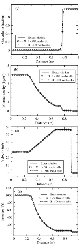
1.4 and π = 0. Two simulations of water-air shock tube were conducted using different mesh resolutions. In the first simulation, curve (I), both fluids are governed by SG EOS and in the second simulation, curve (II), water is governed by SG EOS and air is governed by van der Waals EOS. Figure 1 shows the results of volume fraction (a), mixture density (b), velocity (c) and pressure (d) using 500 cells compared to the exact solution at timet= 229µs. It can be observed that the shock position obtained in the first simulation, curve (I), is closer to the exact solution than that obtained in the second simulation, curve (II). Table I gives the computational costs for both simulations using different mesh cells. It can be seen that at mesh resolution of 2000 and higher van der Waals EOS needs more CPU time than SG EOS to obtain the solution. Also, it can be seen that van der Waals EOS needs more time steps than SG EOS to obtain the solution for all mesh resolutions.
B. Gas-air Shock Tube Test
0 0.2 0.4 0.6 0.8 1 Distance (m)
0 0.2 0.4 0.6 0.8 1
Gas volume fraction
Exact solution I - 500 mesh cells II - 500 mesh cells (a)
0 0.2 0.4 0.6 0.8 1
Distance (m) 0
200 400 600 800 1000 1200
Mixture density (kg/m
3 )
Exact solution I - 500 mesh cells II - 500 mesh cells (b)
0 0.2 0.4 0.6 0.8 1
Distance (m) 0
100 200 300 400 500
Velocity (m/s)
Exact solution I - 500 mesh cells II - 500 mesh cells (c)
0 0.2 0.4 0.6 0.8 1 Distance (m)
0 2e+08 4e+08 6e+08 8e+08 1e+09 1.2e+09
Pressure (Pa)
Exact solution I - 500 mesh cells II - 500 mesh cells
(d)
Fig. 1. Water-air shock tube results: curve (I) water and air are governed by SG EOS, curve (II) water is governed by SG EOS and air is governed by van der Waals EOS.
m. The gas on the left side is given an initial velocity to the right. The initial conditions, taken from [19], are as follows:
(ρ, u, p) =
3.984, 27.355, 1000 ifx≤0.2
0.01, 0.0, 1 ifx >0.2
A strong shock wave with a pressure ratio of 1000 propagates from a high density gas to a low density gas. The constant parameters for both EOSs for air are as given in the previous test. The SG EOS parameters for the gas on the left side are γ= 1.667andπ= 0. Two simulations of gas-air shock tube were conducted using different mesh resolutions. In the first simulation, curve (I), both gases are governed by SG EOS,
TABLE II
THE TIME STEPS AND THECPURUN TIME FOR GAS-AIR SHOCK TUBE, (I)GAS AND AIR ARE GOVERNED BYSG EOS, (II)GAS IS GOVERNED
BYSG EOSAND AIR IS GOVERNED BY VAN DERWAALSEOS.
I II
Mesh Time step CPU time (s) Time step CPU time (s)
100 665 0 665 0
200 1343 0 1343 0
500 3351 2 3351 2
1000 6697 10 6697 10
2000 13389 40 13389 42
5000 33465 250 33465 263
while in the second simulation, curve (II), gas is governed by SG EOS and air is governed by van der Waals EOS. Figure 2 shows the results of volume fraction (a), mixture density (b), velocity (c) and pressure (d) using 500 cells compared to the exact solution at time t = 0.01 s. It can be noticed that both simulations are identical. Table II gives the computational costs for both simulations of gas-air shock tube using different mesh cells. It can be seen that at mesh resolution of 2000 and higher van der Waals EOS needs more CPU time than SG EOS to obtain the solution. But both EOSs need the same time steps to obtain the solution for all mesh resolutions.
C. Water-faucet Test
This test has been used to show the ability of this compressible model to solve incompressible flows. It was proposed by Ransom [20]. The test consists of a 12m vertical tube that contains a water column that is surrounded by air. Water leaves the faucet atvo= 10 m/s andαo= 0.8under
the effect of gravity and the water narrows as it moves down. The velocity relaxation process is not performed because each fluid has a different velocity direction. The initial conditions are as follows
(ρ, u, p, α) = (
1000, 10, 105, 0.8
Water 1, 0, 105
, 0.2 Air (13)
Tait’s and SG EOSs parameters for water areγ= 7.15, B= 3.31×10⁶
Pa and γ = 4.4, π = 6×10⁶
0 0.2 0.4 0.6 0.8 1 Distance (m)
0 0.2 0.4 0.6 0.8 1
Gas volume fraction
Exact solution I - 500 mesh cells II - 500 mesh cells (a)
0 0.2 0.4 0.6 0.8 1
Distance (m) 0
1 2 3 4 5
Mixture density (kg/m
3 )
Exact solution I - 500 mesh cells II - 500 mesh cells (b)
0 0.2 0.4 0.6 0.8 1
Distance (m) 0
10 20 30 40 50 60
Velocity (m/s)
Exact solution I - 500 mesh cells II - 500 mesh cells (c)
0 0.2 0.4 0.6 0.8 1
Distance (m) 0
200 400 600 800 1000 1200
Pressure (Pa)
Exact solution I - 500 mesh cells II - 500 mesh cells
(d)
Fig. 2. Gas-air shock tube results: curve (I) gas and air are governed by SG EOS, curve (II) gas is governed by SG EOS and air is governed by van der Waals EOS.
the following form
L2=
s
PN
i (xi,ex−xi,num)
2
N (14)
where the subscriptsexandnumdenote the values obtained from the exact solution and the numerical solution respec-tively, andNis the number of mesh cells. Figure 5 (a) shows the error norm of gas volume fraction for the four simulations using different mesh cells; the accuracy of all simulations, curves (I), (II), (III) and (IV), is the same for all resolutions
0 2 4 6 8 10 12
Distance (m) 0.1
0.2 0.3 0.4 0.5
Gas volume fraction
Exact solution 100 mesh cells 200 mesh cells 500 mesh cells 1000 mesh cells 1500 mesh cells (a)
0 2 4 6 8 10 12
Distance (m) 9
10 11 12 13 14 15
Water velocity (m/s)
Exact solution 100 mesh cells 200 mesh cells 500 mesh cells 1000 mesh cells 1500 mesh cells
(b)
Fig. 3. Water-faucet results using different mesh resolutions both fluids are governed by SG EOS: (a) gas volume fraction and (b) water velocity.
TABLE III
THE TIME STEPS AND THECPURUN TIME FORWATER-FAUCET, (I) WATER AND AIR ARE GOVERNED BYSG EOS, (II)WATER IS GOVERNED
BYSG EOSAND AIR IS GOVERNED BY VAN DERWAALSEOS.
I II
Mesh Time step CPU time (s) Time step CPU time (s)
100 2130 0 2133 0
200 4257 1 4263 1
500 10639 8 10860 9
1000 21276 30 22108 37
1500 31915 69 33472 83
except at 1500 cells where Tait’s EOS produces overshot with Both SG and van der Waals EOSs for air, curves (III) and (IV). Figure 5 (b) shows that the error norm of water velocity is the same for all simulations for all mesh cells. Tables III and IV give the computational costs for the four simulations of water-faucet test using different mesh cells. It can be seen that SG and Tait’s EOS for water need the same number of time steps and CPU time to obtain the solution but van der Waals EOS needs more number of time steps and CPU time than SG EOS for air to obtain the solution for relatively higher mesh.
V. CONCLUSION
0 2 4 6 8 10 12 Distance (m)
0.1 0.2 0.3 0.4 0.5
Gas volume fraction
Exact solution A - 500 mesh cells B - 500 mesh cells C - 500 mesh cells D - 500 mesh cells (a)
0 2 4 6 8 10 12
Distance (m) 9
10 11 12 13 14 15
Water velocity (m/s)
Exact solution A - 500 mesh cells B - 500 mesh cells C - 500 mesh cells D - 500 mesh cells
(b)
Fig. 4. Water-faucet (a) for volume fraction (b) for water velocity. Curve (I) water and air are governed by SG EOS, curve (II) water is governed by SG EOS and air is governed by van der Waals EOS, curve (III) water is governed by Tait’s EOS and air is governed by SG EOS, curve (IV) water is governed by Tait’s EOS and air is governed by van der Waals EOS.
0 500 1000 1500 2000
Number of mesh cells 0.01
0.02 0.03 0.04
L2
volume fraction error norm
I II III IV
(a)
0 500 1000 1500 2000
Number of mesh cells 0
0.05 0.1 0.15 0.2 0.25
L2
veocity error norm
I II III IV (b)
Fig. 5. Water-faucetL2error norm (a) for volume fraction (b) for water
velocity. Curve (I) water and air are governed by SG EOS, curve (II) water is governed by SG EOS and air is governed by van der Waals EOS, curve (III) water is governed by Tait’s EOS and air is governed by SG EOS, curve (IV) water is governed by Tait’s EOS and air is governed by van der Waals EOS.
accuracy and are in good agreement in all simulations with the exact and the reference results.
TABLE IV
THE TIME STEPS AND THECPURUN TIME FORWATER-FAUCET, (III) WATER IS GOVERNED BYTAIT’SEOSAND AIR IS GOVERNED BYSG EOS, (IV)WATER IS GOVERNED BYTAIT’SEOSAND AIR IS GOVERNED
BY VAN DERWAALSEOS.
III IV
Mesh Time step CPU time (s) Time step CPU time (s)
100 2130 0 2133 0
200 4257 1 4263 1
500 10638 8 10866 9
1000 21274 30 22124 37
1500 31912 69 33500 83
REFERENCES
[1] M. R. Bear and J. Nunziato, “A two-phase mixture theory for the de-flagration to detonation transition DDT in reactive granular materials,”
Int. J. Multiphase Flow, vol. 12, pp. 861–889, 1986.
[2] D. A. Drew, “Mathematical modeling of two-phase flow,” Annual review of fluid mechanics, vol. 15, pp. 261–291, 1983.
[3] R. Saurel and R. Abgrall, “A multiphase Godunov method for com-pressible multifluid and multiphase flows,”Journal of Computational Physics, vol. 150, no. 2, pp. 425– 467, 1999.
[4] G. Allaire, S. Clerc, and S. Kokh, “A five-equation model for the numerical simulation of interfaces in two-phase flows,” Comptes Rendus de l’ Academie des Sciences Paris - Series I: Mathematics, vol. 331, no. 12, pp. 1017–1022, 2000.
[5] A. K. Kapila, R. Menikoff, and D. Stewart, “Two-phase modeling of deflagration-to-detonation transition in granular materials: Reduced equations,”Physics of Fluids, vol. 13, no. 10, pp. 3002–3024, 2001. [6] A. Murrone and H. Guillard, “A five equation reduced model for
compressible two phase flow problems,” Journal of Computational Physics, vol. 202, pp. 664–698, 2005.
[7] H. B. Stewart and B. Wendroff, “Two phase flow: Models and methods,” Jornal of Computaional Physics, vol. 56, pp. 363–409, 1984.
[8] R. Abgrall and S. Karni, “Computations of compressible multifluids,”
J. Comput. Phys., vol. 169, pp. 594–623, 2001.
[9] R. Saurel and O. LeMetayer, “A multiphase model for compressible flows with interfaces, shocks,detonation waves and cavitation,”Journal of fluid mechanics, vol. 431, pp. 239–271, 2001.
[10] R. Scardovelli and S. Zaleski, “Direct numerical simulation of free-surface and interfacial flow,” Annu. Rev. Fluid Mech., vol. 31, p. 567603, 1999.
[11] G. Tryggvason, B. Bunner, A. Esmaeeli, D. Juric, N. Al-Rawahi, W. Tauber, J. Han, S. Nas, and J. Y. J., “A front-tracking method for the computations of multiphase flow,”J. Comput. Phys., vol. 169, p. 708759, 2001.
[12] K. Shyue, “A fluid-mixture type algorithm for compressible multi-component flow with van der Waals equation of state,” Journal of Computational Physics, vol. 156, pp. 43–88, 1999.
[13] K. M. Shyue, “A fluid-mixture type algorithm for compressible mul-ticomponent flow with Mie-Gr¨uneisen equation of state,”Journal of Computational Physics, vol. 171, pp. 678–707, 2001.
[14] R. Saurel, E. Franquet, E. Daniel, and O. Le Metayer, “A relaxation-projection method for compressible flows. part I: The numerical equation of state for the Euler equations,”Journal of Computational Physics, vol. 223, no. 5, pp. 822–845, 2007.
[15] H. W. Zheng, C. Shu, Y. T. Chew, and N. Qin, “A solution adaptive simulation of compressible multi-fluid flows with general equation of state,” International Journal for Numerical Methods in Fluids, vol. DOI:10.1002/fld, 2010.
[16] M. Ishii, Thermo-fluid dynamic theory of two-phase flow. Paris: Eyrolles, 1975, vol. 22.
[17] R. Saurel, F. Petitpas, and R. Abgrall, “Modelling phase transition in metastable liquids: application to cavitating and flashing flows,”
Journal of Fluid Mechanics, vol. 607, pp. 313–350, 2008. [Online]. Available: http://dx.doi.org/10.1017/S0022112008002061
[18] M. H. Lallemand, A. Chinnayya, and O. LeMetayer, “Pressure re-laxation procedures for multiphase compressible flows,”International Journal for Numerical Methods in Fluids, vol. 49, no. 1, pp. 1–56, 2005.
[19] X. Y. Hu and B. C. Koo, “An interface interaction method for compressible multifluids,”J. Comput. Phys., vol. 198, pp. 35–64, 2004. [20] V. H. Ransom,Numerical benchmark tests, In Multiphase Science and