Components of variation of polygenic systems with digenic epistasis

(1)

INTRODUCTION

Breeders can assess the potential of base populations for their use in breeding programs and the selection effi-ciency by assessing the relative importance of the addi-tive, dominance and epistatic effects in determining each important trait, as well as choosing the selective proce-dure that will maximize genetic gain with one or more se-lection cycles. In a polygenic system, additive effects are effects which are individually attributable to genes deter-mining a quantitative trait. The existence of differences between the additive genetic values of the individuals in a population is a necessary condition for intrapopulational breeding. The viability of a breeding program aimed at de-veloping hybrids depends on the existence of dominance effects, that is the interaction between allelic genes (Hallauer and Miranda Filho, 1988; Falconer and MacKay, 1996).

Epistatic effects are those effects due to interactions between non-allelic genes. Many questions remain as to the importance of epistasis in breeding programs. In cross-pollinated species,in which individual plants possess ho-mozygous and heterozygous genic combinations, what is the importance of additive x additive, additive x dominance and dominance x dominance epistatic effects? If the ob-jective of a breeding program is the development of supe-rior pure lines only additive x additive, additive x additive x additive, etc., epistatic effects can contribute to the supe-riority of a line in relation to the outstanding parent be-cause each population is formed of one homozygous geno-type. If the objective of the program is to develop single, double and three-way crosses, different kinds of epistatic effects can be important to ensure the production of a

su-perior population because the genotype (or each genotype present) has homozygous and heterozygous genic combi-nations.

Inferences regarding the genetic control of quantita-tive traits are made by means of methods that employ lin-ear and quadratic statistics, e.g., means, variances and co-variances. The methods normally employed in determin-ing genetic components of generation means and genotypic variances and covariances do notpermit the assessment of the contribution of epistatic effects or the assessment of their relative importance compared to other effects. In ge-netic studies it is commonly thought that epistatic effects contribute little to the genotypic values of individuals, and that epistatic variance is small or negligible compared to both additive and dominance variance. However, there is evidence from many analyses that epistatic effects cannot always be ignored (Rishipal, 1993; Ramsay et al., 1994; Saha Ray et al., 1994; Rahman et al., 1994; Mgonja et al., 1994; Bartual et al., 1994; Das and Griffey, 1995; Barakat, 1996).

In a theoretical work on the analysis of the genetic effects of several oil palm traits, Baudouin et al. (1995) concluded that “Epistasis effects may contribute substan-tially to population means if the material tested is highly heterozygous, the genetic base is narrow (selected mate-rial or few individuals used) or there is linkage disequilib-rium (due to further selection and insufficient intercross-ing generations.)”, although in the papers published by Balatero et al. (1995), Gingera et al. (1995) and Holtom

et al. (1995) there was no evidence of epistasis. In all cited papers, the methodology used was generation mean analy-sis with first degree epistaanaly-sis, either exclusively or asso-ciated with diallel (Bartual et al., 1994; Mgonja etal., 1994)

METHODOLOGY

Components of variation of polygenic systems with digenic epistasis

José Marcelo Soriano Viana

Abstract

In this paper an extension of the biometric model of Mather and Jinks for the analysis of variation with digenic epistasis is presented. Epistatic effects can contribute favorably to the determination of the genotypic values of selected individuals or families and of superior hybrids. Selection will be inefficient, however, if there is a large number of interacting genes because the epistatic components of the between-family and within-family genotypic variances are very high compared to the portion attributable to the average effects of genes. Selection tends to be efficient when the number of interacting genes is reduced, but this depends on the magnitude of due to dominance and environmental variances. The dominance component (H) and the epistatic component due to interactions between homozygous and heterozygous genic combinations (J) can only be estimated when one or more quadratic statistics from the S3 generation, obtained by randomly mating F2 individuals, are used.

(2)

or triple test cross analysis (Ramsay et al., 1994), or with analysis of variation without epistasis (Holtom et al., 1995; Barakat, 1996). A limitation of generation mean analysis is that the absence of the linear components attributable to epistatic effects does not imply the absence of epistasis, since the linear components of means can be null even when constituent effects are not. In this case, there are both posi-tive and negaposi-tive effects (Mather and Jinks, 1974; Kearsey and Pooni, 1996). This problem reveals the importance of analysis of variation using quadratic statistics in establish-ing inferences on the genetic control of quantitative traits. In some genetic studies it is therefore necessary to take into account the contribution of epistatic effects to the expression of one or more traits under analysis to ob-tain unbiased estimates of the genetic parameters. Mather and Jinks (1974) and Kearsey and Pooni (1996) discusses the effect of epistasis on genotypic variances and covari-ances without considering the estimation of the epistatic components. The present paper is an extension of the model presented by the above authors in which I consider analysis of variation in the presence of first degree epistasis.

COMPONENTS OF VARIATION

The genotypic values of individuals for a digenic sys-tem with epistasis in which the genes have independent as-sortment and two allelic forms (A/a and B/b) are presented in Table I (Mather and Jinks, 1974), where d is the differ-ence between the genotypic value of the homozygote with greatest expression and the mean of the genotypic values of the homozygotes (m), h is the difference between the genotypic value of the heterozygote and m, i is the epi-static effect due to the presence of two homozygous genic combinations in an individual, j is the epistatic effect at-tributable to the presence of one homozygous genic com-bination and one heterozygous genic comcom-bination and l is the epistatic effect due to the presence of two heterozy-gous genic combinations. If P1 and P2 are two homozygous

parents having different allelic genes at the two loci under consideration, regardless of the gene distribution in the parents, the following can be shown:

Variance (V) of the genotypic values of the F2 individuals

is:

V1F2 = (d2a + d2b) + (h2a + h2b) + (i2ab) +

+ (j2

ab + j2ba) + (12ab) + (dajab + dbjba) +

Variance of the genotypic means of the F3 families is:

V1F3 = (d2a + d2b) + (h2a + h2b) + (i2ab) +

+ (j2

+ (ha1ab + hb1ab)

Mean of the variances of the genotypic values of the indi-viduals in the same F3 family is:

V2F3 = (d2a + d2b) + (h2a + h2b) + (i2ab) +

+ (j2

+ (ha1ab + hb1ab)

Covariance (W) between the genotypic value of the F2

in-dividual and the genotypic mean of its F3 family is:

W1F23 = (d2a + d2b) + (h2a + h2b) + (i2ab) +

+ (j2

+ (ha1ab + hb1ab)

Variance of the genotypic means of the S3 biparental

fami-lies (obtained by the random mating of F2 individuals) is:

V1S3 = (d2a + d2b) + (h2a + h2b) + (i2ab) +

+ (j2

+ (ha1ab + hb1ab)

Mean of the variances of the genotypic values of the indi-viduals in the same S3 biparental family is:

V2S3 = (d2a + d2b) + (h2a + h2b) + (i2ab) +

+ (j2

+ (ha1ab + hb1ab)

Covariance between the mean of the genotypic values of the F2 parents and the genotypic mean of their S3 biparental

family is:

W1S23 = (d2a + d2b) + (i2ab) + (j2ab + j2ba) +

+ (dajab + dbjba)

Variance of the genotypic means of the groups of F4

fami-Table I - Possible genotypes of two loci.

BB Bb bb

AA m + da + db + iab m + da + hb + jab m + da - db - iab

Aa m + ha + db + jba m + ha + hb + lab m + ha - db - jba

aa m - da + db - iab m - da + hb - jab m - da - db + iab

4 1

+ (ha1ab + hb1ab)

2 1

4 1

16 3

2 1

4 1

16 1

256 3

4 1

32 1

4 1

8 1

16 5

64 3 8

1

8 1

16 1

2 1

8 1

4 1

8 1

64 3

8 3

32 3

4 1

16 1

64 5

256 9

4 1

16 1

4 1

16 3

64 11

256 39

4 1

16 3

4 1

16 1

(3)

lies (the F4 progenies in a group have a common F2

ances-tor) is:

V1F4 = (d2a + d2b) + (h2a + h2b) + (i2ab) +

+ (j2

+ (ha1ab + hb1ab)

Mean of the variances of the genotypic means of the prog-enies in the same group of F4 families is:

V2F4 = (d2a + d2b) + (h2a + h2b) + (i2ab) +

+ (j2

+ (ha1ab + hb1ab)

Mean of the variances of the genotypic values of the indi-viduals in the same F4 family is:

V3F4 = (d2a + d2b) + (h2a + h2b) + (i2ab) +

+ (j2

+ (ha1ab + hb1ab)

Covariance between the genotypic mean of the F3 progeny

and the genotypic mean of its F4 family group is:

W1F34 = (d2a + d2b) + (h2a + h2b) + (i2ab) +

+ (j2

+ (ha1ab + hb1ab)

Mean of the covariances between the genotypic value of an F3 individual and the genotypic mean of its F4 progeny in

the same group of F4 families is:

W2F34 = (d2a + d2b) + (h2a + h2b) + (i2ab) +

+ (j2

+ (ha1ab + hb1ab)

Covariance between the genotypic value of an F2 individual

and the genotypic mean of its F4 family group (covariance

between the genotypic value of the F2 parent and the

geno-typic mean of its F4 descendants) is:

W1F24 = (d2a + d2b) + (h2a + h2b) + (i2ab) +

+ (j2

+ (ha1ab + hb1ab)

Variance of the genotypic values of the F3 individuals is:

VF3 = V1F3 + V2F3

Variance of the genotypic values of the S3 individuals is:

VS3 = V1S3 + V2S3 = V1F2

Variance of the genotypic means of the F4 families is:

VGbF4 = V1F4 + V2F4

Variance of the genotypic values of the F4 individuals is:

VF4 = V1F4 + V2F4 + V3F4

Covariance between the genotypic value of an F3 individual

and the genotypic mean of its F4 family is:

WF34 = W1F34 + W2F34

Let us now consider a polygenic system with interac-tion between genic combinainterac-tions of two loci and genes with independent assortment. If there are allelic differences for all loci among the initial parents, then:

V1F2 = D + H + I + J + L + DJ + HL

V1F3 = D + H + I + J + L + DJ + HL

V2F3 = D + H + I + J + L + DJ + HL

W1F23 = D + H + I + J + L + DJ + HL

V1S3 = D + H + I + J + L + DJ + HL

V2S3 = D + H + I + J + L + DJ + HL

W1S23 = D + I + J + DJ

V1F4 = D + H + I + J + L + DJ + HL

V2F4 = D + H + I + J + L + DJ + HL

V3F4 = D + H + I + J + L + DJ + HL

(4)

where: D = ∑d2

r is a parameter determined by the sum of the

squares of the deviations between the genotypic value of the homozygote with greatest expression and the mean of the homozygotes, for each locus of a poly-genic system, and is a function of the additive effects; H = ∑h2

r is a parameter determined by the sum of the

squares of the deviations between the genotypic value of the heterozygote and the mean of the homozygotes, in relation to each locus of a polygenic system, and is a function of the dominance effects;

I = ∑∑i2

rs (r < s) is a parameter determined by the sum

of the squares of the epistatic effects between two homozygous genic combinations (additive x additive epistatic component);

J = ∑∑ j2

rs (r ≠ s) is a parameter determined by the sum

of the squares of the epistatic effects between a ho-mozygous genic combination and a heterozygous genic combination (additive x dominance epistatic component);

L = ∑∑ l2

rs (r < s) is a parameter determined by the sum

of the squares of the epistatic effects between two heterozygous genic combinations (dominance x dominance epistatic component);

DJ =∑∑ dr jrs (r ≠ s) is a parameter determined by the sum

of the products between the d deviation of a locus and the epistatic effect between a homozygous genic combination of the same locus and a heterozygous genic combination;

HL = ∑∑ hr lrs (r ≠ s; lrs = lsr) is a parameter determined by

the sum of the products between the h deviation of a locus and the epistatic effect between the heterozy-gous genic combination of the same locus and an-other heterozygous genic combination.

The genotypic variances of the generations obtained by backcrossing are functions of the described genetic pa-rameters and also of others that depend on the gene distri-bution in the parents.

DISCUSSION

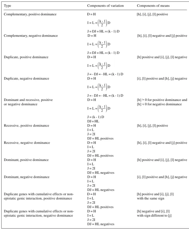
The possible kinds of digenic epistasis are shown in Table II for a polygenic system with k genes. The

param-eters [h], [i], [j] and [l] are due to dominance, additive x additive, additive x dominance and dominance x dominance components of means, respectively (Mather and Jinks, 1974; Kearsey and Pooni, 1996).

In the Fn generation the total (VFn), between-families

(VGbFn) and within-families (VGwFn) genotypic variances can

be expressed in the following way:

VFn =

VGbFn =

VGwFn =

The covariance between the genotypic value of indi-vidual Fn and the mean genotypic value of its progeny Fn + 1

is:

WFn(n + 1) =

After an infinite number of selfing generations,

with-r

W2F34 = D + H + I + J + L + DJ + HL

4 1 16 1 16 5 16 1 256 3 32 3 128 3 2 1 32 1 256 3 1024 3

W1F34 = D + H + I + J + L + DJ + HL

4 1 32 1 16 3 r r s r s r s r s r s

W1F24 = D + H + I + J + L + DJ + HL

16 1 4 1 16 1 256 3 16 5 128 5 2 1 I +

n - 1

1 -2 1      

n - 1

2 1

      J +

22n - 2 - 1 24n - 4

 

 

 

D +

n - 1

1 -2 1

   

  1

-n - 1

2 1

     

n - 1

2 1

      H +

n - 1

1 -2 1       2 L +

n - 1

1 -2 1       +

n - 2

2 1

   

  DJ +

n - 1

1 -2 1

   

  HL

2n - 3

2 1

     

n - 2

1 -2 1       +

n - 2

2 1

   

  DJ +

n - 2

1 -2 1

   

  HL

2n - 2

2 1       D +

n - 2

1 -2 1

   

  1

-n - 2

2 1       n 2 1       H +

n - 2

1 -2 1       2 I +

n - 2

1 -2 1       n 2 1       J +

22n - 4 - 1 24n - 4

 

 

 L +

D +

n - 1

2 1

     

2n - 3 22n - 2

      n 2 1    

  H + I + J +

n

2 1

   

  22n 3

     L +

2n - 2

2 1       DJ + +

2n - 3

2 1

   

  HL

22n - 2 - 1 24n - 2

 

 

 L +

n - 1

1 -2 1       + 2n 3      DJ +

+

n - 1

1 -2 1

   

  22n 3

     HL

+

n - 1

1 -2 1

      I +

2

n - 1

1 -2 1       n 2 1       J +

D +

n - 1

1 -2 1

   

  1

-n - 1

(5)

out selection, mutation, migration or genetic drift, we have:

lim VFn = lim VGbFn = lim WFn(n + 1) = D + I

lim VGwFn = 0

Therefore, as expected, in the generation with an in-breeding coefficient of one (F = 1) the covariance between relatives, the differences between the genotypic values of the individuals in the population and the differences

be-tween the mean genotypic values of the families are due to the differences between the additive genetic values and the additive x additive epistatic values of the individuals. Con-sequently, epistatic effects between homozygous genic combinations can be important in the determination of the superiority of a pure line in relation to the best parent. In breeding programs with self-pollinated plants, the common objective for successive selection cycles is to fix the great-est number of favorable genes in a line. However, the ef-fects of interaction between homozygous genic

combina-Table II - Types of digenic epistasis.

Type Components of variation Components of means

Complementary, positive dominance D = H [h], [i], [j], [l] positive I = L = D

J = DJ = HL = (k - 1) D

Complementary, negative dominance D = H [h], [i], [l] negative and [j] positive I = L = D

J = DJ = HL = (k - 1) D

Duplicate, positive dominance D = H [h] positive and [i], [j], [l] negative I = L = D

J = - DJ = - HL = (k - 1) D

Duplicate, negative dominance D = H [i], [l] positive and [h], [j] negative I = L = D

J = - DJ = - HL = (k - 1) D

Dominant and recessive, positive D = H [h] > 0 for positive dominance and

or negative dominance [h] < 0 for negative dominance

I = L = D J = (k - 1) D DJ = HL

Recessive, positive dominance D = H [h], [i], [j], [l] positive I = L

J = 2I

DJ = HL positives

Recessive, negative dominance D = H [h], [i], [l] negative and [j] positive I = L

J = 2I

DJ = HL positives

Dominant, positive dominance D = H [h] positive and [i], [j], [l] negative I = L

J = 2I

DJ = HL negatives

Dominant, negative dominance D = H [i], [l] positive and [h], [j] negative I = L

J = 2I

DJ = HL negatives

Duplicate genes with cumulative effects or non- D = H [h] positive and [i], [j], [l] epistatic genic interaction, positive dominance I = L with the same sign

J = 2I

DJ = HL positives

Duplicate genes with cumulative effects or non- D = H [h] negative and [i], [l] epistatic genic interaction, negative dominance I = L with sign different to [j]

J = 2I

DJ = HL negatives       k - 1

2       k - 1

2

      k - 1

2

      k - 1

2

      k - 1

2

n →∞ n →∞ n →∞

(6)

tions of desirable genes can contribute in a negative way to the genotypic value of a selected line. If favorable genes increase trait expression and the component [i] is positive, the additive x additive epistatic effects contribute to the superiority of a pure line in relation to the outstanding par-ent. The same is true when the genes of interest decrease trait expression and the component [i] is negative.

Differently to the quadratic components of variation, which are always greater than or equal to zero, the compo-nents DJ and HL can be negative. The sign of the compo-nent DJ is determined by the signs of the additive x domi-nance epistatic effects (j). When positive, it can be con-cluded that epistatic effects due to interactions between homozygous and heterozygous genic combinations are pre-dominantly positive, evidence of complementary genic action or recessive epistasis or dominant and recessive epistasis or duplicate genes with cumulative effects or non-epistatic genic interaction, the last two with positive domi-nance. If the additive x dominance effects are most nega-tive, DJ will be less than zero, indicating duplicate genic action or dominant and recessive epistasis or dominant epistasis or duplicate genes with cumulative effects or non-epistatic genic interaction, the last two with negative domi-nance. When there is no additive x dominance epistatic ef-fects, then DJ = 0.

As the dominance effects (h) and the epistatic effects between heterozygous genic combinations (l) can be nega-tive, null or posinega-tive, if the component HL is positive it can be concluded that these effects should be predominantly positive or negative, indicating complementary genic ac-tion or recessive epistasis or dominant and recessive epista-sis or duplicate genes with cumulative effects or non-epi-static genic interaction, the last two with positive domi-nance. When HL is negative, there is evidence that the domi-nance and domidomi-nance x domidomi-nance effects have opposite signs, an indication of duplicate genic action or dominant and recessive epistasis or dominant epistasis or duplicate genes with cumulative effects or non-epistatic genic inter-action, the last two with negative dominance. If there are no dominance or dominance x dominance epistatic effects, then HL is zero.

Considering that the objective of a breeding program is intrapopulational breeding or hybrid development, epi-static effects between favorable homozygous genic com-binations and heterozygous genic comcom-binations, as well as between heterozygous genic combinations themselves, are causes of covariance between relatives and of genetic vari-ability in the populations. Nevertheless, if these effects have a sign different to the additive effects of the favorable genes they contribute negatively to the determination of the ge-notypic values of the individuals, thus limiting the genetic gain.

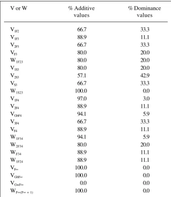
The relative importance of epistatic effects in deter-mining a quantitative trait can be assessed from the analy-sis of the values presented in Tables III to IX. Table III shows the percentage of various genotypic variances and

covari-ances attributable to differences between the additive and dominance genetic values of individuals in the population, assuming complete dominance and the absence of epista-sis. Independent of the number of genes and the genera-tions involved, differences between the individuals in rela-tion to their additive genetic values always determine the major part of the genotypic variance and covariance when compared to the proportion attributable to deviations due to dominance, this being true even when there is epistasis (see Tables IV to IX). The difference between fractions at-tributable to additive and dominance effects increases as the population approaches homozygosis. In comparison to the values in Table III, the percentage attributable to the differences between the additive genetic values will be greater if there is partial dominance and less if there is overdominance.

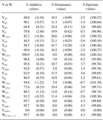
Assuming deviations d of approximately the same magnitude, if there is complementary genic action or re-cessive epistasis, as the number of interacting genes in-creases the greater is the proportion of genotypic variances and covariances due to epistatic effects (Table IV). The same is true when there is duplicate genic action or domi-nant epistasis, also assuming dr≅ d for each dr(r = 1, ..., k) (Table V). For the last two types of epistasis, since the com-ponents DJ and HL are negative and have a high magnitude, compared to D, H, I and L, the values of many genotypic variances and covariances in initial segregant generations can be negative if the number of interacting genes is the

Table III - Percentage of genotypic variances (V) and covariances (W) attributable to differences between additive and dominance genetic

values, assuming complete dominance and absence of epistasis.

V or W % Additive % Dominance

values values

V1F2 66.7 33.3

V1F3 88.9 11.1

V2F3 66.7 33.3

VF3 80.0 20.0

W1F23 80.0 20.0

V1S3 80.0 20.0

V2S3 57.1 42.9

VS3 66.7 33.3

W1S23 100.0 0.0

V1F4 97.0 3.0

V2F4 88.9 11.1

VGbF4 94.1 5.9

V3F4 66.7 33.3

VF4 88.9 11.1

W1F34 94.1 5.9

W2F34 80.0 20.0

WF34 88.9 11.1

W1F24 88.9 11.1

VF∞ 100.0 0.0

VGbF∞ 100.0 0.0

VGwF∞ 0.0 0.0

(7)

same as those in the polygenic system. Even when the num-ber of genes that interact is reduced the total contribution of the epistatic components to genotypic variances and covariances is negative, decreasing their values.

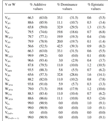
In the case of dominant and recessive epistasis, it is not possible to assume that these types of interaction will occur for each pair of genes. In relation to any three of the genes in a polygenic system (e.g., A/a, B/b and C/c), this kind of epistasis is only possible for two pairs of genes (e.g., A/a and B/b, A/a and C/c), while for the third pair (B/ b and C/c) epistasis is complementary or duplicate. Tables VI and VII show that the contribution of epistatic effects to genotypic variances and covariances is proportional to the number of interacting genes, and that as these increase the greater is the percentage of genotypic variances and covariances due to differences between epistatic genetic values.

In the case of duplicate genes with cumulative effects or non-epistatic genic interaction (both with positive domi-nance), if the number of interacting genes is reduced and epistatic effects are of insignificant magnitude compared to deviations d, the greater part of genotypic variances and covariances will be attributable to differences between the additive genetic values of the individuals, a situation favor-ing selection (Table VIII). As the epistatic effects approach the values of the deviations d, the fractions of the geno-typic variances and covariances due to differences between the additive, dominance and epistatic genetic values will be close to those for complementary epistasis (Table IV). When this is true for duplicate genes with cumula-tive effects and non-epistatic genic interaction (with nega-tive dominance) the values approach those seen for dupli-cate epistasis (Table V). Note that for these types of epista-sis the contribution of the epistatic components to geno-typic variances and covariances in segregant generations is negative (Table IX). An extreme situation occurs when all

k genes in a polygenic system interact: in the initial gen-erations the genotypic variances and covariances are nega-tive because of the values of the DJ and HL components.

If the number of genes that interact approaches the number of genes in the polygenic system the differences between epistatic genetic values of the individuals account for approximately 100% of the genotypic variances and covariances regardless of the type of epistasis, the genera-tion and the relative values of the epistatic effects. The consequences are low, close to zero, heritability at indi-vidual and family levels (even in advanced generations), inefficient selection, and biased estimates of the additive and dominance components and consequently of heritabil-ity, predicted genetic gains, proportions of lines superior to the outstanding parent and other genetic parameters, if the additive-dominance model is adjusted.

On the other hand, if the proportion of interacting genes is reduced, independently of the predominant kind of epistasis, it can be expected that as the population ap-proaches homozygosis the percentage of the genotypic Table IV - Percentage of genotypic variances (V) and covariances

(W) attributable to differences between additive, dominance and epistatic genetic values, assuming complementary genic action or recessive epistasis (dr≅ d), 1000 genes, 10 and 1000

(values in parentheses) interacting.

V or W % Additive % Dominance % Epistatic

values values values

V1F2 58.2 (0.04) 29.1 (0.02) 12.7 (99.94)

V1F3 82.6 (0.11) 10.3 (0.01) 7.1 (99.88)

V2F3 59.6 (0.05) 29.8 (0.03) 10.6 (99.92)

VF3 73.2 (0.08) 18.3 (0.02) 8.5 (99.90)

W1F23 72.3 (0.07) 18.1 (0.02) 9.6 (99.91)

V1S3 71.0 (0.06) 17.8 (0.01) 11.2 (99.93)

V2S3 49.3 (0.03) 36.9 (0.02) 13.8 (99.95)

VS3 58.2 (0.04) 29.1 (0.02) 12.7 (99.94)

W1S23 89.0 (0.07) 0.0 (0.00) 11.0 (99.93)

V1F4 92.6 (0.19) 2.9 (0.01) 4.5 (99.80)

V2F4 82.1 (0.10) 10.2 (0.01) 7.7 (99.89)

VGbF4 88.8 (0.14) 5.6 (0.01) 5.6 (99.85)

V3F4 60.4 (0.06) 30.2 (0.03) 9.4 (99.91)

VF4 83.2 (0.12) 10.4 (0.01) 6.4 (99.87)

W1F34 88.8 (0.14) 5.5 (0.01) 5.7 (99.85)

W2F34 72.8 (0.07) 18.2 (0.02) 9.0 (99.91)

WF34 82.7 (0.11) 10.3 (0.01) 7.0 (99.88)

W1F24 81.8 (0.09) 10.2 (0.01) 8.0 (99.90)

VF∞ 95.7 (0.20) 0.0 (0.00) 4.3 (99.80)

VGbF∞ 95.7 (0.20) 0.0 (0.00) 4.3 (99.80)

VGwF∞ 0.0 (0.00) 0.0 (0.00) 0.0 (0.00)

WF∞(F∞ + 1) 95.7 (0.20) 0.0 (0.00) 4.3 (99.80)

Table V - Percentage of genotypic variances (V) and covariances (W) attributable to differences between additive, dominance

and epistatic genetic values assuming duplicate genic action or dominant epistasis (with dr≅ d), 1000 genes, 10

and 1000 (values in parentheses) interacting.

V1F2 69.0 (-0.18) 34.5 (-0.09) -3.5 (100.27)

V1F3 90.1 (-0.57) 11.3 (-0.07) -1.4 (100.64)

V2F3 64.8 (0.21) 32.4 (0.11) 2.8 (99.68)

VF3 79.8 (2.48) 19.9 (0.62) 0.3 (96.90)

W1F23 82.3 (-0.26) 20.6 (-0.06) -2.9 (100.32)

V1S3 84.5 (-0.13) 21.1 (-0.03) -5.6 (100.16)

V2S3 58.3 (-0.26) 43.7 (-0.20) -2.0 (100.46)

VS3 69.0 (-0.18) 34.5 (-0.09) -3.5 (100.27)

W1S23 106.0 (-0.16) 0.0 (0.00) -6.0 (100.16)

V1F4 96.8 (4.00) 3.0 (0.10) 0.2 (95.90)

V2F4 85.6 (0.21) 10.7 (0.03) 3.7 (99.76)

VGbF4 92.8 (0.57) 5.8 (0.04) 1.4 (99.39)

V3F4 62.9 (0.10) 31.5 (0.05) 5.6 (99.85)

VF4 86.9 (0.35) 10.9 (0.04) 2.2 (99.61)

W1F34 94.8 (-1.22) 5.9 (-0.08) -0.7 (101.30)

W2F34 77.6 (0.23) 19.4 (0.06) 3.0 (99.71)

WF34 88.3 (1.12) 11.0 (0.14) 0.7 (98.74)

W1F24 91.2 (-0.32) 11.4 (-0.04) -2.6 (100.36)

VF∞ 95.7 (0.20) 0.0 (0.00) 4.3 (99.80)

VGbF∞ 95.7 (0.20) 0.0 (0.00) 4.3 (99.80)

VGwF∞ 0.0 (0.00) 0.0 (0.00) 0.0 (0.00)

(8)

Table VI - Percentage of genotypic variances (V) and covariances (W) attributable to differences between additive, dominance and

epistatic genetic values, assuming dominant and recessive epistasis, 300 and 30 genes (values in parentheses), 3 interacting,

and complementary genic action for one pair.

V1F2 65.4 (55.9) 32.7 (28.0) 1.9 (16.1)

V1F3 88.0 (80.6) 11.0 (10.1) 1.0 (9.3)

V2F3 65.4 (55.7) 32.7 (27.9) 1.9 (16.4)

VF3 78.9 (70.2) 19.7 (17.5) 1.4 (12.3)

W1F23 78.9 (70.3) 19.7 (17.6) 1.4 (12.1)

V1S3 78.8 (69.7) 19.7 (17.4) 1.5 (12.9)

V2S3 55.9 (46.7) 41.9 (35.1) 2.2 (18.2)

VS3 65.4 (55.9) 32.7 (28.0) 1.9 (16.1)

W1S23 98.6 (87.6) 0.0 (0.0) 1.4 (12.4)

V1F4 96.3 (90.5) 3.0 (2.8) 0.7 (6.7)

V2F4 87.6 (77.2) 10.9 (9.7) 1.5 (13.1)

VGbF4 93.2 (85.6) 5.8 (5.3) 1.0 (9.1)

V3F4 65.4 (55.7) 32.7 (27.8) 1.9 (16.5)

VF4 87.8 (79.5) 11.0 (9.9) 1.2 (10.6)

W1F34 93.3 (86.8) 5.8 (5.4) 0.9 (7.8)

W2F34 78.7 (68.5) 19.7 (17.1) 1.6 (14.4)

WF34 87.9 (79.7) 11.0 (10.0) 1.1 (10.3)

W1F24 87.9 (80.1) 11.0 (10.0) 1.1 (9.9)

VF∞ 99.0 (90.9) 0.0 (0.0) 1.0 (9.1)

VGbF∞ 99.0 (90.9) 0.0 (0.0) 1.0 (9.1)

VGwF∞ 0.0 (0.0) 0.0 (0.0) 0.0 (0.0)

WF∞(F∞ + 1) 99.0 (90.9) 0.0 (0.0) 1.0 (9.1)

Table VII - Percentage of genotypic variances (V) and covariances (W) attributable to differences between additive, dominance and epistatic genetic values, assuming dominant and recessive epistasis,

300 and 30 (values in parentheses) genes, 3 interacting, and duplicate genic action for one pair.

V1F2 66.3 (63.0) 33.1 (31.5) 0.6 (5.5)

V1F3 88.6 (85.9) 11.1 (10.7) 0.3 (3.4)

V2F3 65.8 (59.0) 32.9 (29.5) 1.3 (11.5)

VF3 79.5 (74.6) 19.8 (18.6) 0.7 (6.8)

W1F23 79.7 (77.1) 19.9 (19.3) 0.4 (3.6)

V1S3 79.9 (78.9) 20.0 (19.7) 0.1 (1.4)

V2S3 56.6 (52.5) 42.5 (39.3) 0.9 (8.2)

VS3 66.3 (63.0) 33.1 (31.5) 0.6 (5.5)

W1S23 99.9 (99.2) 0.0 (0.0) 0.1 (0.8)

V1F4 96.6 (93.4) 3.0 (2.9) 0.4 (3.7)

V2F4 87.8 (79.5) 11.0 (10.0) 1.2 (10.5)

VGbF4 93.5 (88.3) 5.8 (5.5) 0.7 (6.2)

V3F4 65.6 (57.3) 32.8 (28.6) 1.6 (14.1)

VF4 88.2 (82.0) 11.0 (10.2) 0.8 (7.8)

W1F34 93.8 (91.0) 5.9 (5.7) 0.3 (3.3)

W2F34 79.0 (71.5) 19.8 (17.9) 1.2 (10.6)

WF34 88.3 (83.4) 11.0 (10.4) 0.7 (6.2)

W1F24 88.6 (86.6) 11.1 (10.8) 0.3 (2.6)

VF∞ 99.0 (90.9) 0.0 (0.0) 1.0 (9.1)

VGbF∞ 99.0 (90.9) 0.0 (0.0) 1.0 (9.1)

VGwF∞ 0.0 (0.0) 0.0 (0.0) 0.0 (0.0)

WF∞(F∞ + 1) 99.0 (90.9) 0.0 (0.0) 1.0 (9.1)

Table IX - Percentage of genotypic variances (V) and covariances (W) attributable to differences between additive, dominance and epistatic genetic values, assuming duplicate genes with cumulative

effects (with irs = i) or non-epistatic genic interaction (with dr = d

and irs = i), 1000 genes, 10 and 1000 (values in parentheses)

interacting, i = 0.1d, and negative dominance. V or W % Additive % Dominance % Epistatic

V1F2 67.2 (-0.7) 33.6 (-0.4) -0.8 (101.1)

V1F3 89.3 (-2.0) 11.1 (-0.2) -0.4 (102.2)

V2F3 66.9 (-1.6) 33.5 (-0.8) -0.4 (102.4)

VF3 80.3 (-1.8) 20.1 (-0.5) -0.4 (102.3)

W1F23 80.5 (-1.1) 20.1 (-0.3) -0.6 (101.4)

V1S3 80.7 (-0.8) 20.2 (-0.2) -0.9 (101.0)

V2S3 57.6 (-0.6) 43.2 (-0.5) -0.8 (101.1)

VS3 67.2 (-0.7) 33.6 (-0.4) -0.8 (101.1)

W1S23 100.9 (-1.0) 0.0 (0.0) -0.9 (101.0)

V1F4 97.2 (-4.6) 3.0 (-0.1) -0.2 (104.7)

V2F4 89.0 (-5.2) 11.1 (-0.6) -0.1 (105.8)

VGbF4 94.3 (-4.7) 5.9 (-0.3) -0.2 (105.0)

V3F4 66.7 (-4.5) 33.4 (-2.2) -0.1 (106.7)

VF4 89.1 (-4.7) 11.1 (-0.6) -0.2 (105.3)

W1F34 94.4 (-2.8) 5.9 (-0.2) -0.3 (103.0)

W2F34 80.2 (-2.7) 20.1 (-0.7) -0.3 (103.4)

WF34 89.2 (-2.8) 11.1 (-0.3) -0.3 (103.1)

W1F24 89.4 (-1.5) 11.2 (-0.2) -0.6 (101.7)

VF∞ 99.9 (16.7) 0.0 (0.0) 0.1 (83.3)

VGbF∞ 99.9 (16.7) 0.0 (0.0) 0.1 (83.3)

VGwF∞ 0.0 (0.0) 0.0 (0.0) 0.0 (0.0)

WF∞(F∞ + 1) 99.9 (16.7) 0.0 (0.0) 0.1 (83.3) Table VIII - Percentage of genotypic variances (V) and covariances

(W) attributable to differences between additive, dominance and epistatic genetic values, assuming duplicate genes with cumulative effects (with irs = i) or non-epistatic genic interaction

(with dr = d and irs = i), 1000 genes, 10 and 1000 (values in

parentheses) interacting, i = 0.1d, and positive dominance. V or W % Additive % Dominance % Epistatic

V1F2 66.0 (0.6) 33.0 (0.3) 1.0 (99.1)

V1F3 88.5 (1.6) 11.0 (0.2) 0.5 (98.2)

V2F3 66.3 (1.1) 33.2 (0.6) 0.5 (98.3)

VF3 79.6 (1.4) 19.9 (0.4) 0.5 (98.2)

W1F23 79.4 (1.0) 19.9 (0.2) 0.7 (98.8)

V1S3 79.3 (0.8) 19.8 (0.2) 0.9 (99.0)

V2S3 56.6 (0.5) 42.4 (0.4) 1.0 (99.1)

VS3 66.0 (0.6) 33.0 (0.3) 1.0 (99.1)

W1S23 99.1 (1.0) 0.0 (0.0) 0.9 (99.0)

V1F4 96.7 (3.4) 3.0 (0.1) 0.3 (96.5)

V2F4 88.6 (2.7) 11.1 (0.3) 0.3 (97.0)

VGbF4 93.9 (3.1) 5.9 (0.2) 0.2 (96.7)

V3F4 66.5 (1.9) 33.2 (1.0) 0.3 (97.1)

VF4 88.6 (2.9) 11.1 (0.3) 0.3 (96.8)

W1F34 93.8 (2.3) 5.9 (0.1) 0.3 (97.6)

W2F34 79.7 (1.8) 19.9 (0.4) 0.4 (97.8)

WF34 88.5 (2.0) 11.1 (0.3) 0.4 (97.7)

W1F24 88.4 (1.3) 11.0 (0.2) 0.6 (98.5)

VF∞ 99.9 (16.7) 0.0 (0.0) 0.1 (83.3)

VGbF∞ 99.9 (16.7) 0.0 (0.0) 0.1 (83.3)

VGwF∞ 0.0 (0.0) 0.0 (0.0) 0.0 (0.0)

(9)

variances and covariances attributable to the differences between the additive genetic values of the individuals be-comes relatively high (the superior limit of heritability), while other factors become less important, and conse-quently the efficiency of family and mass selection is in-creased. In the F3 and F4 generations the efficiency of

within-family selection is practically the same, subsequently reducing as the inbreeding coefficient approaches 1. Heri-tability at a family level tends to be greater than that at the individual level, and, disregarding environmental effects, the analysis of the values presented in Tables III to IX shows the superiority of family selection in comparison to mass selection, except when F = 1, in which case these different types of selection are equivalent. If the total and within-family environmental variances are of approximately the same magnitude, the superiority of mass selection in rela-tion to the selecrela-tion between plants within families is also evident because heritability at the level of individuals in the population tends to be greater than that at the level of individuals within families.

An important aspect of the model presented in this paper, which needs to be further studied, is that the estima-tion of the genetic components of variaestima-tion D, H, I, J, L,

DJ and HL, depends on the inclusion of at least one vari-ance associated with the S3 generation and/or of the

cova-riance W1S23, since in the genotypic variances and

covari-ances of selfing generations the coefficients of the com-ponents H and J are the same. Therefore, if only estimates of the variances and covariances of selfing generations are available, only the components D, (H + J), I, L, DJ and HL, are estimable. The estimation of (H + J) may not be limit-ing since the two components are due to genic effects not transmitted from generation to generation and they do not contribute to the expected genetic gain due to selection, tending to disappear when the inbreeding coefficient in the population approaches one. However, the calculation of the average degree of dominance and other H-dependent pa-rameters is not possible. The estimation of the genetic and non-heritable components can be based on the weighted or ordinary least squares method (Mather and Jinks, 1974) or on the maximum likelihood method (Hayman, 1960).

The analysis of variation by the additive-dominance model with epistasis allows an assessment of the relative importance of epistatic effects in the genetic control of a trait, and favors an unbiased estimation of the additive (D) and dominance (H) components and of other genetic pa-rameters that depend on these effects. For a better under-standing of the control of a quantitative trait, information from the generation mean analysis, including epistasis, can be associated with information from the analysis of varia-tion.

A comparative assessment of the linear components [d], [h], [i], [j] and [l] with the corresponding quadratic com-ponents should permit the clarification of the relative im-portance of additive, dominance and epistatic genic effects, and allow us to decide if non-additive effects are

predomi-nantly uni- or bidirectional and whether or not favorable genes are concentrated in one parent, as well as to eluci-date the prevailing type of epistasis, etc., all of which al-low a better planning of breeding programs.

If the objective of a breeding program is to develop superior lines, the magnitude of the epistatic components [i] and I and the sign of the former should be assessed. The analysis should permit us to infer whether or not fixation of favorable genes is associated with fixation of desirable epistatic effects due to the interaction between homozy-gous genic combinations increasing genetic gain. If the aim is to develop a hybrid, then it is necessary to analyze the contribution of the genetic effects represented by the pa-rameters [h], H, [i], I, [l] and L, to select for heterosis (“hy-brid vigor”) in the desired direction, with greater heterosis being expected when such effects are predominantly di-rectional.

CONCLUSIONS

If the additive x additive, additive x dominance and dominance x dominance epistatic effects have the same sign as the average effects of desirable genes, they contribute favorably to the determination of the genotypic values of selected individuals, families or hybrids. Nevertheless, if there is a large number of interacting genes the percentage due to epistatic effects of the total, between-family and within-family genotypic variances is very high in compari-son to the portion attributable to the average effects of the genes, making the identification of the superior individu-als or families inefficient. In this case, analysis according to the additive-dominance model will produce very biased estimates of genetic parameters. Depending on the magni-tude of the dominance and environmental variances, when the number of interacting genes is reduced selection tends to be efficient and the fit with the additive-dominance model should be reasonable. The model for analysis of variation presents multicollinearity.

RESUMO

(10)

REFERENCES

Balatero, C.H., Darvey, N.L. and Luckett, D.J. (1995). Genetic analysis of anther-culture response in 6x triticale. Theor. Appl. Genet.90: 279-284.

Barakat, M.N. (1996). Estimation of genetic parameters for in vitro traits in wheat immature embryo cultures involving high X low regeneration capacity genotypes. Euphytica87: 119-125.

Bartual, R., Lacasa, A., Marsal, J.I. and Tello, J.C. (1994). Epistasis in the resistance of pepper to phytophthora stem blight (Phytophthora capsici L.) and its significance in the prediction of double cross per-formances. Euphytica72: 149-152.

Baudouin, L., Cao, T.V. and Gallais, A. (1995). Analysis of the genetic effects for several traits in oil palm (Elaeis guineensis Jacq.) popula-tions. I. Population means. Theor. Appl. Genet.90: 561-570.

Das, M.K. and Griffey, C.A. (1995). Gene action for adult-plant resistance to powdery mildew in wheat. Genome38: 277-282.

Falconer, D.S. and MacKay, T.F.C. (1996). Introduction to Quantitative Genetics. 4th edn. Longman, Essex.

Gingera, G.R., Davis, D.W. and Groth, J.V. (1995). Identification and in-heritance of delayed first pustule appearance to common leaf rust in sweet corn. J. Am. Soc. Hortic. Sci.120: 667-672.

Hallauer, A.R. and Miranda Filho, J.B. de (1988). Quantitative Genetics in Maize Breeding. 2nd edn. Iowa State University Press, Ames.

Hayman, B.I. (1960). Maximum likelihood estimation of genetic

compo-nents of variation. Biometrics16: 369-381.

Holtom, M.J., Pooni, H.S., Rawlinson, C.J., Barnes, B.W., Hussain, T.

and Marshall, D.F. (1995). The genetic control of maturity and seed characters in sunflower crosses. J. Agric. Sci.125: 69-78.

Kearsey, M.J. and Pooni, H.S. (1996). The Genetical Analysis of Quantita-tive Traits. Chapman and Hall, London.

Mather, K. and Jinks, J.L. (1974). Biometrical Genetics. 2nd edn. Cornell University Press, Ithaca, New York.

Mgonja, M.A., Ladeinde, T.A.O. and Aken’ova, M.E. (1994). Genetic analy-sis of mesocotyl length and its relationship with other agronomic characters in rice (Oryza sativa L.). Euphytica72: 189-195.

Rahman, H., Wicks, Z.W., Swati, M.S. and Ahmed, K. (1994). Generation mean analysis of seedling root characteristics in maize (Zea mays L.).

Maydica39: 177-181.

Ramsay, L.D., Bradshaw, J.E. and Kearsey, M.J. (1994). The inheritance of quantitative traits in Brassica napus ssp. rapifera (swedes): augmen-ted triple test cross analysis of yield. Heredity73: 84-91.

Rishipal, K.P. (1993). Generation mean analysis of yield and yield attri-butes in Indian mustard (Brassica juncea). Indian J. Agric. Sci.63: 807-813.

Saha Ray, P.K., Hillerislambers, D. and Tepora, N.M. (1994). Genetics of stem elongation ability in rice (Oryza sativa L.). Euphytica74: 137-141.