www.hydrol-earth-syst-sci.net/15/1921/2011/ doi:10.5194/hess-15-1921-2011
© Author(s) 2011. CC Attribution 3.0 License.
Earth System
Sciences
Data-driven catchment classification: application to the pub
problem
M. Di Prinzio, A. Castellarin, and E. Toth
DICAM – Department of Civil and Environmental Engineering - University of Bologna, Viale Risorgimento 2, 40136 Bologna, Italy
Received: 23 December 2010 – Published in Hydrol. Earth Syst. Sci. Discuss.: 18 January 2011 Revised: 11 May 2011 – Accepted: 6 June 2011 – Published: 23 June 2011
Abstract. A promising approach to catchment classifica-tion makes use of unsupervised neural networks (Self Or-ganising Maps, SOM’s), which organise input data through non-linear techniques depending on the intrinsic similarity of the data themselves. Our study considers∼300 Italian catchments scattered nationwide, for which several descrip-tors of the streamflow regime and geomorphoclimatic char-acteristics are available. We compare a reference classifi-cation, identified by using indices of the streamflow regime as input to SOM, with four alternative classifications, which were identified on the basis of catchment descriptors that can be derived for ungauged basins. One alternative clas-sification adopts the available catchment descriptors as in-put to SOM, the remaining classifications are identified by applying SOM to sets of derived variables obtained by ap-plying Principal Component Analysis (PCA) and Canonical Correlation Analysis (CCA) to the available catchment de-scriptors. The comparison is performed relative to a PUB problem, that is for predicting several streamflow indices in ungauged basins. We perform an extensive cross-validation to quantify nationwide the accuracy of predictions of mean annual runoff, mean annual flood, and flood quantiles asso-ciated with given exceedance probabilities. Results of the study indicate that performing PCA and, in particular, CCA on the available set of catchment descriptors before applying SOM significantly improves the effectiveness of SOM clas-sifications by reducing the uncertainty of hydrological pre-dictions in ungauged sites.
Correspondence to:A. Castellarin
(attilio.castellarin@unibo.it)
1 Introduction
A common problem in hydrology is the prediction in un-gauged basins of the streamflow regime (e.g., long-term mean value and variability of streamflows, flood flows as-sociated with a given exceedance probability, low-flow in-dices, etc.). The scientific literature has often highlighted the remarkable natural variability of geomorphological char-acteristics of basins and of their hydrological behavior for different climatic inputs. This consideration motivated the pursuit of general laws in hydrology to be used for predict-ing the hydrologic behavior of ungauged basins on the basis of historical data.
This issue is eloquently stated by Dooge (1986) in the well known work “Looking for hydrologic laws”, but, at the same time, it is also the central topic of many recent inter-national scientific initiatives, such as the Prediction in Un-gauged Basins (PUB) of the International Association of Hy-drological Sciences (IAHS) (see e.g., Sivapalan et al., 2003). The scientific community states that little progress has been made in this field in the last two decades and indicates that the formulation of objective criteria for catchment classifica-tion is one of the main objectives for obtaining a better in-terpretation and representation of spatiotemporal variability of streamflows (McDonnell and Woods, 2004; McDonnell et al., 2007; Bai et al., 2009).
(see e.g., Bardossy, 2007; Yadav et al., 2007; Castiglioni et al., 2010), which is also is particularly relevant to the PUB-problem.
A very interesting and promising approach to tion makes use of an innovative and data-driven classifica-tion method based on unsupervised artificial neural networks (ANNs), known as Self Organising Maps (SOM, Kohonen, 1982, Toth, 2009; Ley et al., 2011).
As in previous recent studies (Hall and Minns, 1999; Jungy and Hall, 2004; Srinivas et al., 2008), the main goal of our study is to assess whether SOM classifications may be effectively utilized for reducing the uncertainty of hydrolog-ical predictions in ungauged basins.
The element of novelty of this study consists in the in-tegration of SOM techniques with two multivariate analy-sis techniques that reduce the original high-dimensionality of geomorphoclimatic pattern information, namely the Prin-cipal Component Analysis (PCA) and Canonical Correlation Analysis (CCA) (see e.g., Krzanowski, 1988; Ouarda et al., 2001). It has been shown for other disciplines that integrat-ing PCA and CCA improves the practical usability of SOM classifications (see Yan et al., 2001). Our study aims at un-derstanding if integrating PCA and CCA with SOM can also be a useful resource in the PUB context.
Our study considers a national database counting 296 Ital-ian unregulated catchments compiled within the national re-search project “CUBIST – Characterisation of Ungauged Basins by Integrated uSe of hydrological Techniques” (Claps and the Cubist Team, 2008). The streamflow regime and the physiographic and climatic characteristics of the study catch-ments are summarised by several catchment descriptors. The background idea is the identification of a multipurpose catch-ment classification that could, in principle, serve different hy-drological analyses and be used for addressing different PUB problems (for example design flood estimation or assessment of long-term surface water availability).
We identify a Reference Classification (RC) of the study catchments to be compared with four Alternative Classifi-cations (AC’s) in the context of PUB. RC results from the application of SOM to a set of descriptors of the streamflow regime, whereas AC’s are identified on the basis of catch-ment descriptors that are commonly available for ungauged basins. The first AC adopts a set of geomorphoclimatic de-scriptors as input to SOM. The remaining AC’s are identified by applying SOM to three sets of derived variables obtained by applying PCA (second AC) and CCA (third and fourth AC’s) to the available geomorphoclimatic descriptors.
First, the similarity between each AC and RC is as-sessed qualitatively, analysing how the study catchments were grouped together. Second, AC’s are compared with RC in terms of accuracy of streamflow prediction. To this aim, AC’s and RC are used as basis to regionalise several streamflow indices. In order for the comparison to be fair we adopted the same regionalization approach for all clas-sifications, and we performed an extensive cross-validation
procedure to quantify nationwide the accuracy of estimates of the mean annual flow, mean annual flood, and flood quan-tiles associated with given exceedance probabilities.
2 Catchment classification and som
2.1 Literature review
A catchment may be defined as the area which drains nat-urally to a particular point on a river or stream. Catch-ments are very complex systems, these landscape eleCatch-ments can have different sizes and characteristics. In general it is hard to identify an appropriate classification system that may have general applicability. The recent emphasis on catch-ment classification highlights the need for methodical criteria to classify catchments and their hydrological behaviour (Mc-Donnell and Woods, 2004). To date, hydrologists have not reached a consensus on a classification system (McDonnell et al., 2007; Wagener et al., 2007).
Regionalization procedures are generally based on the def-inition of hydrologically homogeneous regions or pooling groups of sites. Regionalization is a commonly used ap-proach for predicting streamflow regimes in ungauged basins (see e.g., Castellarin et al. 2001, 2004; Castellarin, 2007).
The majority of the pioneering studies on catchment clas-sification and hydrological regionalization adopted the geo-graphic contiguity criterion. Nevertheless, very soon the sci-entific community urged for a globally agreed upon classi-fication system, based on the variability of physical and cli-matic characteristics of the catchments (Acreman and Sin-clair, 1986) and identifiable by means of objective method-ologies (i.e., cluster analysis, Burn, 1989).
In recent years a number of techniques based on various mathematical approaches have been proposed by the liter-ature. A very interesting and promising approach to clas-sification makes use of unsupervised artificial neural net-works (ANN) (see e.g., Hall and Minns, 1999). Over the last decades ANN’s have been subject to an increasing in-terest in a variety of practical applications. The increasing number of applications of ANN’s is related to their ability to relate input and output variables in complex systems without any requirement of a detailed understanding of the physics of the process involved (Dawson and Wilby, 2001). The unsu-pervised ANN differ from suunsu-pervised ANN, which are more commonly used in hydrology, because they do not focus on the identification of a relationship between input and output variables. They organize input data through non-linear tech-niques depending on their similarity instead.
2.2 SOM networks and catchment classification
Maps (SOM’s, Kohonen, 1982; 1997) are an unsupervised learning method to analyze, cluster, and model various types of large databases. The SOM method counts sev-eral hydrological applications (see e.g., Kalteh et al., 2008; C´er´eghino and Park, 2009), such as classification of hydro-logical and meteorohydro-logical conditions for streamflow fore-casting (Toth, 2009). SOM networks cluster groups of sim-ilar input patterns from a high dimensional input space in a non-linear fashion onto a low dimensional (most com-monly two-dimensional for representation and visualization purposes) discrete lattice of neurons in an output layer (Ko-honen, 2001; Kalteh et al., 2008).
Typically a SOM consists of two layers, an input layer and a Kohonen or output layer (see Fig. 1 after Kalteh et al., 2008). The input layer contains one neuron for each vari-able (i.e., catchment attribute) in the data set. The number of classes (i.e., neurons of the output layer) is generally prede-fined by the modeller and the classes themselves are ordered into meaningful maps that preserve the topology (see Kalteh et al., 2008). The output-layer neurons are connected to ev-ery neuron in the input layer through adjustable weights (see Fig. 1), whose values are identified through an iterative train-ing procedure. Lateral interaction between neighbourtrain-ing out-put nodes ensures that learning is a topology-preserving pro-cess in which the network adapts to respond in different lo-cations of the output layer for inputs that differ, while similar input patterns activate units that are close together. Following a random initialisation of the weight vectors, SOM utilizes a type of learning that is calledcompetitive,unsupervised, or
self-organizing procedure to match each input vector with
only one neuron in the output layer. This is done by compar-ing the presented input pattern with each of the SOM neuron weight vectors, on the basis of a distance measure, like the Euclidean distance. The neuron with the closest match to the presented input pattern is called winner neuron. Then, the weight vector of the winner neuron and of the topologically neighbouring neurons are updated in such a way as to repro-duce the input pattern (see e.g., Kalteh et al., 2008 and Toth, 2009 for further details).
Once trained (calibrated), the network activates only one output node in correspondence of each input vector. There-fore, all input vectors activating the same node belong to the same class.
3 Multivariate analysis for dimensionality reduction
3.1 Principal Component Analysis – PCA
The Principal Component Analysis, PCA (see e.g., Krzanowski, 1988), is a multivariate analysis statistical method that enables one to obtain smaller number of uncor-related variables from a larger number of possibly coruncor-related variables by constructing an orthogonal basis for the origi-nal variables themselves. The derived uncorrelated variables
Fig. 1. Structure of a 5×5 two-dimensional self organizing map
(SOM) (after Kalteh et al., 2008).
are called principal components (PC). The full set of PC’s has the same dimensionality of the original set of variables. They are ordered in such a way that the first component ac-counts for as much of the variability in the original dataset as possible, and each following PC accounts for as much of the remaining variability as possible.
It is commonplace for the sum of the variances of the first few PCs to exceed 80 % of the total variance of the origi-nal data. By examining plots of these few new variables, researchers often develop a deeper understanding of the driv-ing forces that generated the original data. The literature re-ports several criteria for selecting the appropriate number of principal components (see e.g. Kaiser, 1960 criterion and the scree plot).
3.2 Canonical Correlation Analysis – CCA
Another important multivariate statistical tool for reducing the dimensionality of the original dataset is the Canonical Correlation Analysis (CCA). The multivariate approach of CCA is most commonly used in the context where there are two sets of random multidimensional and correlated vari-ables X={X1,X2,. . . ,Xn} and Y={Y1,Y2,. . . ,Ym} (e.g.,
ge-omorphoclimatic catchment descriptors and indices of the streamflow regime, such as the annual flow, the flood as-sociated with a given recurrence interval, etc.). CCA en-ables one to identify the dominant linear modes of covari-ability between the sets X and Y (see e.g., Krzanowski,
1988; Ouarda et al., 2001). In other words, CCA identifies two new groups of artificial variables (canonical variables)
U={U1,U2,. . . ,Ur}andV={V1,V2,. . . ,Vr}, withr=min{n,m},
by finding linear combinations of the original Xi, with i=1,. . . ,n, andYj, withj=1,. . . ,m, in such a way that the
correlation between the canonical variables of a pair (Ui,Vi)
Table 1.Minimum, mean and maximum values, and 25th, 50th and 75th percentiles for the set ofXvariables considered in the study. These data were either derived from a SAR-DTM (Synthetic Aperture Radar – Digital Terrain Model) with grid size 100 m or * retrieved from Rep. no 17 of the former Italian SIMN (National Hydrographic Service of Italy).
long. lat. A P zmax zmin zmean L SL SA 8 MAP*
(m) (m) (km2) (km) (m a.s.l.) (km) (%) (%) (deg.N.) (mm)
Minimum 319 450 4 170 550 3.2 8.0 284 3.0 127.0 2.6 1.8 6.2 0.7 602.0
Mean 704 261 4 752 661 1060.8 157.8 2092 342.0 986.7 54.8 10.1 29.1 186.6 1224.2 Maximum 1 162 850 5 195 450 17 512.1 1115.0 4727 1812.0 3110.0 357.9 35.4 63.0 359.3 2289.0
25th 505 825 4 545 450 98.0 52.75 1409 77.7 567.5 18.7 5.3 18.4 73.9 960.75
50th 680 450 4 814 250 331.0 102.5 1814 231.5 838.5 35.9 8.5 26.8 204.0 1152.5
75th 897 475 4 922 150 930.7 187.25 2625 462.5 1242.7 66.1 13.6 38.5 276.8 1410.0
If we denote byXandY the independent and dependent
variables respectively and we consider the linear transforma-tions,
U=uT
X·XandV=u
T
Y·Y (1)
characterized by the basis vectorsuX anduY, CCA can be
defined as the following optimization problem, ρ= max
uX,vY{
corr(U,V)} = max
uX,vY
cov(U,V)
√
var(U)√var(V). (2)
4 Study area and available information
The study area consists of 296 Italian catchments scattered nationwide, whose dataset was compiled within the national research project “CUBIST – Characterisation of Ungauged Basins by Integrated uSe of hydrological Techniques” (see e.g., Claps et al., 2008), and is definitely heterogeneous in terms of climatic and geomorphologic characteristics that control the streamflow regime.
4.1 Geomorphoclimatic and streamflow variables
We refer to 12 different geomorphological and climatic de-scriptors of the study catchments, which we term in the study X variables, and 6 descriptors of the streamflow regime, which we termY variables.
Xvariables:
– (1 and 2) long. and lat. – UTM longitude and latitude of catchment centroid;
– (3)A– Drainage area; – (4)P – Perimeter;
– (6)zmax– Highest elevation;
– (6)zmin– Elevation of the catchment outlet;
– (7)zmean– Mean altitude;
– (8)L– Maximum drainage length;
– (9) SL – Average slope along the maximum drainage
length;
– (10)SA– Catchment average slope;
– (11)8– Catchment orientation; – (12) MAP – Mean Annual Precipitation; Y variables:
– (1) MAR – Mean Annual Runoff;
– (from 2 to 5)li – sample L moments of orderi=1 (i.e.,
sample mean), 2, 3 and 4 of the annual maximum series AMS of flood flows (see e.g., Hosking, 1990);
– (6) REC/l1– Ratio between the maximum value and the
sample mean of AMS of flood flows.
Tables 1 and 2 summariseXandYvariables in terms of min-imum, mean and maximum values, and 25th, 50th and 75th percentiles for the set of 296 considered catchments.
-0.6 -0.4 -0.2 0 0.2 0.4 0.6
long. lat. A P z
max zmin zmean L SL SA φ MAP
PC1 PC2 PC3
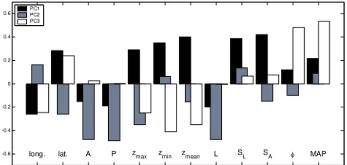
Fig. 2. Coefficients of the linear transformation for the first three
PC’s of theXvariables.
4.2 Application of PCA and CCA
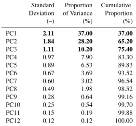
We reduced the dimensionality of the 12-dimensional space of the geomorphoclimatic descriptors (X variables) and the 6-dimensional space of the streamflow regime descriptors (Y variables) through the application of PCA and CCA. In par-ticular we computed all PC’s ofX variables relative to the whole set of 296 basins. As said before, the full set of PC’s is as large as the original set of variables. The 12 PC’s have zero mean and a decreasing standard deviation (see Table 3), but the most interesting property is that the first three prin-cipal components explain roughly the two third of the total variability, in this case more than the 75.4 % (Table 3).
Figure 2 reports the coefficients of linear transformation of eachX variable for the first three Principal Components. This information is explained from the eigenvalues calcu-lated for our dataset.
Likewise, we applied the CCA to the set ofXandY vari-ables relative to the whole of the 296 study basins. As re-ported above, the number of canonical variables is equal to the smallest dimension of the two sets of variables, in our case theYvariables. Therefore we obtained 6 canonical vari-ables for each set,UandV.
The scatter-plots of Fig. 3 illustrate the relationships be-tween the canonical variablesU(x-axis) andV(y-axis) com-puted for the study area, also illustrating, as expected, a sig-nificant correlation between the first canonical variablesUi
andVi. Table 4 shows the significance of the null
hypothe-sis that all correlation coefficients betweenUj andVj– with j=i,. . . r=6 – are zero. As Table 4 shows, the first 4 canoni-cal variables are the most descriptive for the problem at hand. As done for PC’s, we report in Fig. 4 the coefficients of lin-ear transformation associated with eachXvariable for all six components ofU.
5 Comparison of som classifications of the study catchments
There are no predefined classes of the conditions character-ising the basin: a clustering algorithm is here used as an
Fig. 3. Canonical variables U and V computed for the study
area: scatter-plots between canonical variablesUiandVj, foriand
jequal to 1,2,. . . 6.
-3 -2.5 -2 -1.5 -1 -0.5 0 0.5 1 1.5 2
Variables X
long. lat. A P z
max zmin zmean L SL SA φ MAP
U1 U2 U3 U4
Fig. 4. Coefficients of the linear transformation for the canonical
variables of theXvariables.
unsupervised classifier, where the task is to learn a
classi-fication from the data. Such partitioning will be based on the most relevant available information, that is, descriptors of the streamflow regime and geomorphoclimatic character-istics. Our study identifies several classifications on the ba-sis of different sets of catchment descriptors (Sect. 5.1) by implementing different SOM networks (Sect 5.2); we then compare these classifications by looking at the similarity of the partitions (Sect. 5.3) and by assessing the performance of each classification for the prediction of streamflow indices in ungauged basins (Sect. 5.4).
5.1 Reference and alternative SOM classifications
Table 2.Minimum, mean and maximum values, and 25th, 50th and 75th percentiles for the set ofYvariables considered in the study. These data were either computed from the digital database of Italian AMS of flood flows compiled during the Italian VaPi (GNDCI-CNR) project or * retrieved from Rep. no 17 of the former Italian SIMN (National Hydrographic Service of Italy).
MAR* l1 l2 l3 l4 REC/l1
(mm) (m3s−1) (m3s−1) (m3s−1) (m3s−1) (–)
Minimum 84.0 1.0 0.3 −27.3 −32.3 1.2
Mean 780.6 309.0 86.1 21.0 16.5 2.7
Maximum 4406.0 1881.6 584.8 154.6 222.1 9.5
25th 384.7 56.1 17.8 2.6 2.3 1.9
50th 653 163.0 51.7 12.1 9.5 2.5
75th 1080.2 418.0 123.6 29.3 21.7 3.3
Table 3.Principal Components ofXvariables: variability
accounted for.
Standard Proportion Cumulative Deviation of Variance Proportion
(–) (%) (%)
PC1 2.11 37.00 37.00
PC2 1.84 28.20 65.20
PC3 1.11 10.20 75.40
PC4 0.97 7.90 83.30
PC5 0.89 6.53 89.83
PC6 0.67 3.69 93.52
PC7 0.60 3.02 96.54
PC8 0.49 1.98 98.52
PC9 0.28 0.64 99.16
PC10 0.25 0.54 99.70
PC11 0.15 0.19 99.88
PC12 0.12 0.12 100.00
– Reference Classification (RC)
– SOMY is obtained by using indices of the stream-flow regime (Y variables);
– Alternative Classifications (ACs):
– SOMX is based upon the geomorphoclimatic de-scriptors (Xvariables);
– SOMPC3 uses the first three Principal Components of theXvariables;
– SOMU uses all canonical variables computed by applying CCA toXandY variables (i.e.,Ui, with i=1,. . . , 6);
– SOMU4 uses a subset containing the most descrip-tive canonical variables (i.e.,Ui, withi=1,. . . , 4).
5.2 SOM classification implementation
A different SOM network was implemented for each set of catchment characteristics (Y, X, U, U4, PC3). The dimension
Table 4.Canonical Correlation Analysis: level of significanceαof
the null-hypothesis that theiththrough the 6thcorrelations are all zero.
i ρ(Ui,Vi) Significanceα
1 0.900 0.00
2 0.830 0.00
3 0.498 0.00
4 0.362 0.00
5 0.244 0.06
6 0.165 0.34
of the input layer varies from 3 (PC3) to 12 (X). As far as the output layer is concerned, there is not a predefined number of classes and it was here chosen an hexagonal topology formed by three rows by three columns, for a total of nine nodes, each one corresponding to a class.
0.75 0.80 0.85 SOMX
SOMPC3
SOMU
SOMU4
Rand
Index
0.05 0.10 0.15 0.20
SOMX
SOMPC3
SOMU
SOMU4
Adj.
Rand
Index
6 9
3 5
8
2 4
7
1
SOMY
SOMPC3
SOMU4
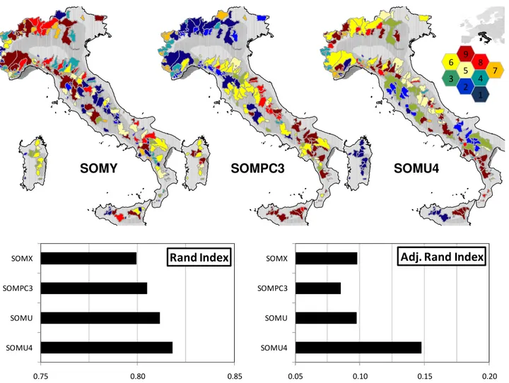
Fig. 5.SOM classifications of the study catchments (note that SOMU is omitted) and hexagonal topology of the output layer; bar-diagram
for Rand and Adjusted Rand Index.
case and deemed nine classes suitable for all classifications (i.e., the one based upon 6Y variables, and those based upon 12X variables and their linear combinations). We used the Euclidean distance as a measure of the distance between the vectors, according to the majority of hydrological applica-tions.
Three out of five SOM’s classifications resulting from the different sets of descriptors are represented in Fig. 5 (SOMX and SOMU were omitted due to space limitations). Note that no relationship exists between classes depicted by the same colour in different classifications.
The three different SOM’s classifications resulted in visi-bly different grouping of the catchments, but also a high level of consistency exists across the three maps, suggesting that groups of landscape-climate similarity are largely indepen-dent of the method of classification used.
A detailed and comprehensive physically based interpre-tation of the patterns emerging from the different classifi-cations is clearly out of the scope of our analysis, which assesses whether (unsupervised and objective) multivariate
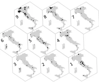
Fig. 6.Reference classification SOMY.
may be noted that classes 8, 6, 5, 4 and 1 can be associ-ated with very clear patterns: class 8 is mainly representative of Northern catchments that, particularly for the Apenninic ones show a high degree of homogeneity in the flood fre-quency regime (see e.g., Castellarin et al., 2001; Castellarin, 2007); catchments belonging to class 6 are predominantly characterized by a maritime regime, the class groups together insular coastal catchments of Sardinia and Sicily, and Io-nian catchments; class 5 includes mainly Apenninic medium catchments characterized by relatively low altitudes; class 4 clusters low-permeability Apenninic catchments (see e.g., Castellarin et al., 2001, 2004); the majority of class 1 catch-ments are located in areas characterized by limestones and sandstones, often fractured, and, for the limestone areas the presence of karst phenomena (ISPRA-DDS, 2004; Castel-larin et al., 2004). Incidentally, it is worth noting that the fact that SOMU4 groups together all Sardinian catchments is a consequence of the rather significant weight longitude and latitude have in the first four canonical variates (see Fig. 4).
Figure 7 compares the SOM classifications in terms of number of basins belonging to each class. The figure reports the sample cumulative distribution functions of the number of basins belonging to the nine classes of each classification, indicating the typical size of each class (average number of basins is equal to 33), together with the variability around the average value. All classifications present similar distri-butions, even though AC’s clearly show a higher degree of similarity among themselves in terms of number of basins in each class. Concerning this point it is worth noting that while RC is identified on the basis of indices characterizing the streamflow regime, all AC’s are delineated by applying SOM techniques to information that can be retrieved for un-gauged basins.
Any ungauged basin, once characterized in terms of the 12 considered catchment descriptors, can be allocated to one of
0 20 40 60 80
-1.5 -1 -0.5 0 0.5 1 1.5
N
um
be
r of
ba
s
ins
Standard normal variate
SOMY SOMX SOMU SOMU4 SOMPC3
Fig. 7. Sample cumulative distribution function of the number of
basins in each class.
the nine classes of each alternative SOM classifications. The regional streamflow information collected within the class to which the ungauged site belongs can then be used to infer the streamflow regime of the ungauged site itself. The next two sections assess the effectiveness of AC’s in terms of (1) affin-ity to the RC and (2) usabilaffin-ity in the PUB context to predict the streamflow regime in ungauged catchment.
5.3 Affinities of alternative SOM classifications with the reference classification
Two indices of similarity were applied to quantify the affini-ties between reference (SOMY) and alternative classifica-tions: the Rand Index (Rand, 1971), RI, and its variation proposed by Hubert and Arabie (1985).
Comparing two partitions (P1 andP2)of the same data
set, a couple of objects (i.e., catchments) can belong to the same class or different classes inP1andP2. Let us define
N00 as the number of catchments that belong to the same
class both inP1 andP2;N10 as the number of catchments
that belong to the same class in P2 but not in P1; N01 as
the number of catchments that belong to the same class inP1
but not inP2;N11as the number of catchments that belong to
different classes both inP1andP2. Under these assumptions,
RI reads,
RI=N N11+N00
11+N00+N10+N01
(3) RI varies between 1 (perfect agreement between the two par-titions) and 0 (no agreement).
Hubert and Arabie (1985) proposed an adjustment to the Rand Index so that its expected value is equal to zero for random partitions having the same number of objects in each class. The index is still equal to 1 for perfect agreement but it can also take negative values (higher discriminatory power than RI).
alternative classification differs from the reference one in terms of number of classes. Also for this reason, we pre-ferred to consider the same number of nodes (i.e., nine) for all SOM classifications to facilitate the comparison.
The bar-diagrams of Fig. 5 show the values obtained for these indices by comparing the RC (i.e., SOMY) with all AC’s (i.e., SOMX, SOMPC3, SOMU and SOMU4). RC is based on the use of hydrometric information, therefore the effectiveness of all AC’s, which are suitable for ungauged basins, is “measured” relative to SOMY.
Figure 5 shows that, as it was expected, SOMX and SOMPC3 are similar to each other in terms of affinity with SOMY. Figure 5 also shows that SOMU and SOMU4 are more similar to SOMY than SOMX and SOMPC3, indi-cating that SOMU4 outperforms all other classifications in terms of affinity with the reference classification SOMY.
These results are a consequence of the intrinsic nature of the alternative SOM classifications considered in our study. SOMX uses all geomorphological and climatic descriptors, therefore there is no direct relationship with the informa-tion used for delineating SOMY and, also, the informainforma-tion utilised to delineate SOMX presents redundancy that may impact the efficiency of the classification process. SOMPC3 uses only the most descriptive portion of the available geo-morphologic and climatic information, therefore removing some noise from the input data, yet there is no direct re-lation with the hydrometric information also in this case. SOMU, instead, uses as input information geomorphologic and climatic information rearranged to maximize the corre-lation with the streamflow regime, and SOMU4 uses only the geomorphologic and climatic information which shows the highest correlation with the streamflow regime.
5.4 Quantitative comparison of SOM classifications in the PUB context
The effectiveness of each classification has been further as-sessed relative to the estimation of streamflow regime for un-gauged sites. To this aim we developed a number of multiple regression models for estimating the streamflow index of in-terest in ungauged sites and we assessed the performances of these models in cross-validation for all AC’s considered in the study, to better understand whether or not the utiliza-tion of PCA and CCA may improve the practical usability of SOM catchment classifications, reducing the uncertainty of predictions in ungauged sites.
For the sake of generality and simplicity, we referred in the study to the simplest possible model structure, there-fore adopting a linear multiregression model as the reference model. The model reads,
ˆ
yi=A0+A1PC1i+A2PC2i+A3PC3i+ϑ (4)
whereA0, A1, A2 and A3 are the parameters of the
mul-tivariate linear regression model; PC1i, PC2i and PC3i are
the first three principal components of variablesXfor sitei,
withi= 1, . . . , 296, which explain more than the 75.4 % of the total variance and, for consistency, are used as explana-tory variables in all multiregression models developed in the study;ϑis the residual of the model; andyˆiis the normalized
streamflow index of interest for sitei, ˆ
yi=ˆ zi− ¯z
sZ
, (5)
withzˆi empirical value of the streamflow index for sitei,
andz¯andsZ empirical mean and standard deviation of the
streamflow index of interest for the entire dataset.
We performed this analysis by developing for each catch-ment classification of interest four different multiregression models (4), namely one model for estimating of Mean An-nual Runoff (MAR) and three models for estimating the first 3 sample L moments of the annual maximum seriesl1, l2
andl3. In particular, four models were identified for RC (i.e.,
SOMY), which represents the optimal classification, and for each of the four AC’s (i.e., SOMX, SOMPC3, SOMU and SOMU4). Four multiple linear regression models were also identified for the entire national set of basins (NOCLASS), which represents a baseline condition in the comparison and sets the minimum level of performance.
We assessed the efficiency of each alternative classifica-tion AC by referring to the results of an extensive jack-knife cross-validation of all 24 regression models developed for the six identified classifications (i.e., RC -optimal-, AC’s, NO-CLASS -baseline-).
The jack-knife cross-validation procedure is applied in or-der to quantify the accuracy of each model when applied in ungauged basins; it is also called in the literature as delete-one or leave-delete-one-out cross-validation procedure (see e.g., Efron, 1982; Zhang and Kroll, 2007; Brath et al., 2003; Castellarin et al., 2004). This method is extremely versatile and capable of providing adequate evaluation of the perfor-mance of the interpolation techniques, since it simulates the ungauged conditions for each site in the study region. The procedure can be illustrated as follows,
1. one catchment is eliminated from the set of N catch-ments;
2. an empirical multiregression model is identified on the basis of the information collected at the N-1 remain-ing catchments (i.e., the first three principal components are computed and the coefficientsAj of (4), withj =
0, . . . , 3, are estimated through linear multiregression techniques);
3. the model developed at step (2) is used for estimating the streamflow index at the discarded site;
4. steps (1) to (3) are repeatedN-1 times, each time by eliminating a different catchment.
account the hydrometric information available at the site itself.
The results of the various cross-validations were quantified in terms of Nash-Sutcliffe efficiency measure (NSE) (Nash and Sutcliffe, 1970). NSE varies in the range ]-∞, 1], where 1 corresponds to a perfect agreement between modelled and empirical values, NSE=0 indicates that estimated values are as accurate as the mean of the observed values, while nega-tive values occur when the observed mean value is a better predictor than the model. The performance index reads
NSE=1−
P
i=1,N
ηJ K,i−ηi
2
P
i=1,N
ηi− P i=1,N
ηi N
!2 (6)
whereηJ K,iindicates the jack-knife estimate andηi the
em-pirical value for sitei, withi=1, . . . ,N.
We computed the performance index relative to jack-knife and empirical values of MAR (Mean Annual Runoff) and l1 (mean annual flood). Producing reliable predictions of
MAR and l1 in ungauged sites is of primary concern (see
e.g., Brath et al., 2001; Castellarin et al., 2004; Kjeldsen and Jones, 2010). Concerning the higher order L moments (i.e., l2andl3), instead of comparing directly empirical and
jack-knife values we preferred to focus on flood quantiles (i.e., flood flows associated with a given recurrence intervalT ), computed on the basis of the L-moments. We deem the flood quantiles to be more meaningful and understandable thanl2
andl3 for summarising the flood frequency regime from a
practical viewpoint. Ultimately, hydrologists and practition-ers are interested in the estimation of the design flood in un-gauged sites rather than the L moments’ values.
We estimated the flood quantiles at each and every site from a Generalized Extreme-Value (GEV) distribution es-timated with the L moments method (GEV-LMOM algo-rithm), which is often more efficient than the maximum like-lihood when used with small to moderate length samples (please refer to Hosking and Wallis, 1997 for details of the frequency distribution and the method of L moments). The GEV distribution was selected in light of its satisfactorily re-production of the sample frequency distribution of hydrolog-ical extremes in Italy and around the world (see e.g., Ste-dinger et al., 1993; Robson and Reed, 1999; Castellarin et al., 2001).
We arbitrarily selected three different return periods, T=10, 50 and 100 years and we estimated the flood quan-tiles through the GEV-LMOM algorithm by referring to the sample L momentsl1,l2andl3and their jack-knife estimates
for all classifications of interest (RC, AC’s, NOCLASS). We then compared these estimates in terms of (6). To avoid un-duly extrapolations, we limited the comparison for T= 10 and 50 yr to the 92 out of 296 sites with at least 30 yr of ob-served annual maxima, and to the 34 out of 296 sites with at least 40 yr of observations forT= 50 and 100 yr.
It is worth highlighting here that even though the use of NSE has become a natural part of the modelling practice, its utilization is still a matter of concern (see e.g., Gupta et al., 2009). In fact, the usefulness of the observed mean as a refer-ence value varies strongly in practical applications. Like all the squared measures, NSE weights the largest observation very heavily at the expense of smaller values, to overcome this problem we computed NSE on logflows, this is typically considered valuable for flood and mean annual streamflows.
6 Results and discussion
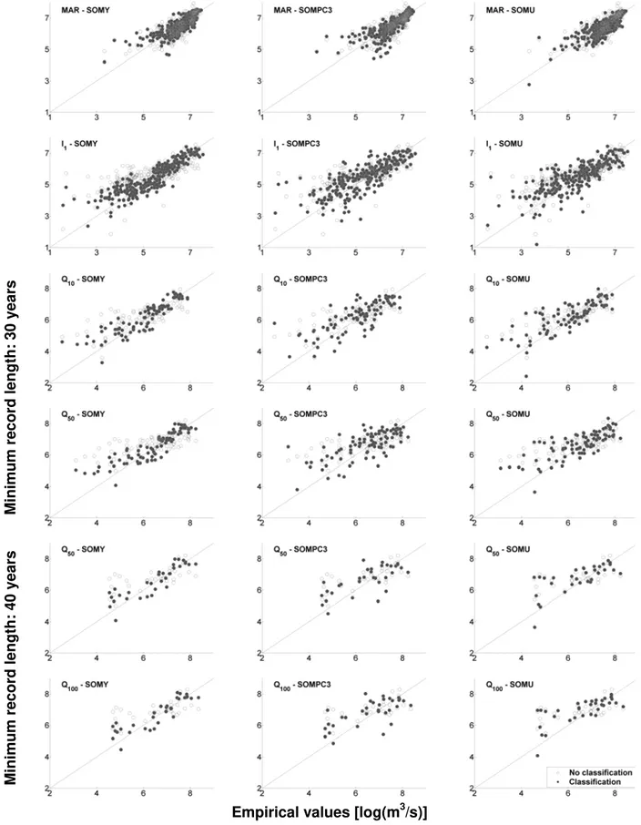
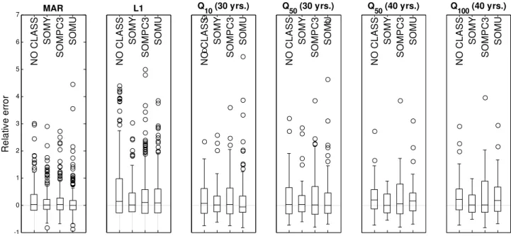
Table 5 reports the values obtained for NSE for all cross-validated streamflow indices and classifications. The scat-ter plots of Fig. 8 report sample estimates of streamflow in-dices of interest against predicted values obtained in cross-validation for some of the classifications considered in the study. Distribution of relative residuals between empirical and jack-knifed values of the streamflow index of interest are illustrated in Fig. 9 for NOCLASS, SOMY, SOMPC3 and SOMU.
The comparison between the results obtained for the base-line condition (NOCLASS) and alternative classifications (i.e., SOMX, SOMPC3, SOMU, SOMU4) indicates that all SOM classifications led to a remarkable improvement in the prediction ability of the considered multiregressive model for all streamflow indices considered in the study. NSE val-ues show significant improvements for all streamflow indices and alternative classifications relative to NOCLASS (see Ta-ble 5). Also, the comparison between the results obtained for SOMX and those relative to SOMPC3, SOMU and SOMU4 points out that combining SOM with PCA or CCA can im-prove effectiveness and usefulness of SOM classifications in the PUB context, that is for predictions of streamflow indices in ungauged basins.
Results reported in Table 5 indicate that multiregression models based on SOMU4 outperform the other models for predicting MAR in ungauged basins. SOMU4 is as accurate as the optimal classification SOMY in predicting MAR in ungauged basins.
Table 5 illustrates a different picture for the prediction of the annual flood (l1). In this case the application of SOMPC3
Table 5.Cross-validation of multiple regression models: NSE values for log-transformed streamflow indices (QT indicates the flood quantile with recurrence intervalT, the highest NSE value among alternative classifications is highlighted in bold-italics).
Minimum NSE
Record Length NO-CLASS SOMY SOMX SOMPC3 SOMU4 SOMU
MAR
No limit 0.53 0.75 0.69 0.66 0.75 0.64
l1 0.49 0.76 0.53 0.58 0.54 0.42
Q10
30 yr 0.52 0.76 0.45 0.55 0.48 0.59
Q50 0.48 0.80 0.45 0.53 0.55 0.61
Q50
40 yr 0.36 0.79 0.34 0.53 0.43 0.49
Q100 0.30 0.82 0.35 0.52 0.47 0.53
Concerning the prediction of flood quantiles, the results of our study point out a clear supremacy of SOMU. Table 5 in-dicates that SOMU is associated with the highest NSE values 3 out of 4 times. It is interesting to note that also SOMPC3 shows good performances, implying that the removal of re-dundant information involved in the identification of SOMX improves the accuracy of the regional models. Nevertheless, the lower bias and variability of residuals of SOMU relative to SOMPC3 is also evident in the boxplots of Fig. 9.
Concerning the box-plots of Fig. 9, a striking figure is the large number of outliers (circles) of relative residuals for the predictions of all streamflow indices considered in cross-validation (outliers are defined as values situated at a distance from the lower and upper quartiles which is 1.5 times larger than the distance between the quartiles themselves). This may be due to the extreme simplicity of the linear regional model and the huge variability of climatic and hydrological characteristics of the consider catchments.
Furthermore, results obtained for SOMY (reference clas-sification) and SOMX, SOMPC3, SOMU4 and SOMU re-ported in Table 5 and Fig. 9 also point out rather clearly that, aside from predictions of MAR, there is still a great margin for improvements. The gap in terms of performance between regional models based on SOMY and models based on all al-ternative classifications is significant. It is worth noting that this outcome has nothing to do with the limitations of the simplistic regional model adopted in the study (i.e., Eq. 4), nor the information used by the regional model. The struc-ture of the regional model does not vary and the predictions in cross-validation of all regional model are based upon the same information (i.e., first three principal components ofX variables). Simply, SOMY transfers the streamflow informa-tion from gauged sites to ungauged ones in a more effective way. None of the catchment classifications based directly (SOMX) or indirectly (SOMPC3, SOMU, SOMU4), on the available catchment descriptors is as efficient as SOMY in transferring the streamflow information from gauged to un-gauged sites. This gap may be reduced by identifying more informative catchment descriptors (see e.g., Savenije, 2010) given the growing availability of easily accessible high
res-olution topographic and land-cover data, together with GIS tools for hydrologic analysis. Further improvements may probably stem from a process-based reorganization of the available information based on physically-based criteria that aims at further removing some noise characterizing the avail-able set of catchment descriptors.
Concerning this point, future analyses could study the variability of catchment characteristics within each class (or node) of the SOM networks, testing whether this variability can be related with the uncertainty in the predicted stream-flow indices. Moreover, future analyses, possibly focussing on larger datasets and diverse climatic and hydrological con-ditions, could further test the same classification algorithm (i.e., PCA/CCA and SOM) for catchment descriptors that combine (1) raw morphological information (e.g., catchment area, main channel and drainage network length, altimetry) to compute hydrologically significant characteristics, such as for instance the time of concentration or drainage density (Pallard et al., 2009), and (2) raw climatic information (e.g., catchment scale mean monthly and annual precipitation and temperature) to estimate aridity indices or net precipitation (Castellarin et al., 2007).
7 Conclusions
Our study analyses the effectiveness of unsupervised neural networks (Self Organising Maps, SOM) coupled with mul-tivariate techniques for reducing the high dimensionality of catchment descriptors (i.e., Principal Component Analysis, PCA, and Canonical Correlation Analysis CCA) for produc-ing catchment classifications on objective bases.
Catchment classification does not have a purpose in itself in the context of our analysis, and does not represent a mere scientific exercise, but represents the means to transfer in-formation from gauged sites to ungauged ones, reducing the uncertainty of hydrological predictions in ungauged sites.
Minimu
m re
cord length:
30 year
s
Jack
-knife v
a
lues [log
(m
3
/s)]
Minimu
m re
cord length:
40 year
s
Empirical values [log(m
3/s)]
816
Fig. 8.Examples of scatter-plots (empirical vs. jack-knife values) obtained in cross-validation for some of the classifications considered in
-1 0 1 2 3 4 5 6 7 R e la tiv e e rro r MAR NO CL ASS SO M Y SO M P C 3 SO M U L1 NO CL ASS SO M Y SO M P C 3 SO M U Q
10 (30 yrs.)
NO CL ASS SO M Y SO M P C 3 SO M U Q
50 (30 yrs.)
NO CL ASS SO M Y SO M P C 3 SO M U Q
50 (40 yrs.)
NO CL ASS SO M Y SO M P C 3 SO M U Q
100 (40 yrs.)
NO CL ASS SO M Y SO M P C 3 SO M U
Fig. 9.Distribution of relative errors in terms of 25th, 50th and 75th percentiles, maximum and minimum values, and outliers (circles).
Mediterranean, from humid to semiarid, and from continen-tal to maritime conditions.
The catchments are grouped into five different classifica-tions, all delineated by means of unsupervised neural net-works. One reference classification is identified by using as catchment descriptors indices of the streamflow regime and flood statistics (reference classification). Four alternative classifications are derived by referring to a number of geo-morphologic and climatic catchment descriptors which can be computed for ungauged basins. One of this classification uses the entire set of descriptors as input variables to SOM, whereas the remaining three alternative classifications utilize as input variables a limited number of measures that are lin-ear combinations of the original catchment descriptors ob-tained by applying PCA or CCA.
We compared the similarity of the alternative classifica-tions with the reference classification. We also compared the accuracy of regional predictions of mean annual runoff, mean annual flood and flood quantiles for various recurrence inter-vals based on the alternative catchment classifications with the accuracy of the same predictions based on (1) the refer-ence classification and (2) a baseline condition which groups together the entire system of Italian catchments (absence of classification). The regional predictions are obtained through the application of an extensive cross-validation procedure that simulates the ungauged conditions at each and every site. Main outcomes of the study may be summarised as fol-lows: (i) SOM’s confirm their effectiveness and usefulness as objective criteria for pattern recognition and, in particu-lar, for delineating catchment classifications; (ii) PCA and CCA can significantly improve the effectiveness and useful-ness of SOM in the context of PUB, that is for reducing the
uncertainty of hydrological predictions in ungauged sites; we strongly encourage to perform PCA, and in particular CCA, on the available set of catchment descriptors before apply-ing SOM; (iii) catchment classification provides a great deal of information for enhancing hydrological predictions in un-gauged basins, yet the application of objective but merely statistical criteria and algorithms (PCA and CCA with SOM) revealed some limitations that may be significantly reduced by switching from data-driven to data- and process-driven catchment classification. Designing a theoretical framework for combining these two different perspectives is an excit-ing open problem for future analyses. Our study focuses on a multipurpose catchment classification, future analyses will also consider hydrological classifications that are identified by focusing on a more specific water-problem, e.g., predic-tion of low-lows, flood flows, or surface water availability, to assess whether or not the same conclusions still hold. Acknowledgements. The study has been partially supported by the Italian Government through its national grants to the programmes on “Advanced techniques for estimating the magnitude and fore-casting extreme hydrological events, with uncertainty analysis” and “Relations between hydrological processes, climate, and physical attributes of the landscape at the regional and basin scales”. Two anonymous reviewers and the handling editor, Peter Troch, are thankfully acknowledged for their very useful comments on a previous version of this paper.
References
Acreman, M. C. and Sinclair, C. D.: Classification of drainage basins according to their physical characteristics and application for flood frequency analysis in Scottland, J. Hydrol., 84(3), 365– 380, 1986.
Bai, Y., Wagener, T., and Reed, P.: A top-down frame-work for watershed model evaluation and selection un-der uncertainty, Environ. Modell. Softw., 24(8), 901-916, doi:10.1016/j.envsoft.2008.12.012, 2009.
B´ardossy, A.: Calibration of hydrological model parameters for ungauged catchments, Hydrol. Earth Syst. Sci., 11, 703–710, doi:10.5194/hess-11-703-2007, 2007.
Brath, A., Castellarin, A., Franchini, M., and Galeati, G.: Estimat-ing the index flood usEstimat-ing indirect methods, Hydrolog. Sci. J., 46(3), 399–418, 2001.
Brath, A., Castellarin, A., and Montanari, A.: Assessing the reliability of regional depth-duration-frequency equations for gaged and ungaged sites, Water Resour. Res., 39(12), 1367, doi:10.1029/2003WR002399, 2003.
Burn, D. H.: Cluster analysis as applied to regional flood frequency, J. Water Res. Pl., 115(6), 567–582, 1989.
Castellarin, A.: Application of probabilistic envelope curves for design-flood estimation at ungaged sites, Water Resour. Res., 43, W04406, doi:10.1029/2005WR004384, 2007.
Castellarin, A., Burn, D. H., and Brath, A.: Assessing the effec-tiveness of hydrological similarity measures for regional flood frequency analysis, J. Hydrol., 241(3–4), 270–285, 2001. Castellarin, A., Galeati, G., Brandimarte, L., Brath, A., and
Monta-nari, A.: Regional flow-duration curve: realiability for ungauged basins, Adv. Water Res., 27(10), 953–965, 2004.
Castiglioni, S., Lombardi, L., Toth, E., Castellarin, A., and Montanari, A.: Calibration of rainfall-runoff mod-els in ungauged basins: a regional maximum likeli-hood approach, Adv. Water Resour., 33(10), 1235–1242, doi:10.1016/j.advwatres.2010.04.009, 2010.
Castiglioni, S., Castellarin, A., Montanari, A., Skøien, J. O., Laaha, G., and Bl¨oschl, G.: Smooth regional estimation of low-flow in-dices: physiographical space based interpolation and top-kriging, Hydrol. Earth Syst. Sci., 15, 715–727, doi:10.5194/hess-15-715-2011, 2011.
C´er´eghino, R. and Park, Y. S.: Review of the Self-Organizing Map (SOM) approach in water resources: Commentary, Envi-ron. Modell. Softw., 24(8), 945–947, 2009.
Chokmani, K. and Ouarda, T. B. M. J.: Physiographical space-based kriging for regional flood frequency estimation at ungauged sites, Water Resour. Res., 40(12), W12514, doi:10.1029/2003WR002983, 2004.
Claps and the CUBIST Team: Development of an Information Sys-tem of the Italian basins for the CUBIST project, Geophysical Research Abstracts, 10, 2008.
Dawson, C. W. and Wilby, R. L.: Hydrological modelling using ar-tificial neural networks, Prog. Phys. Geog., 25(1), 80–108, 2001. Dooge, J. C. I.: Looking for hydrologic laws, Water Resour. Res.,
22(9), 46–58, 1986.
Efron, B.: The Jackknife the Bootstrap and Other Resampling Plans. Society for Industrial and Applied Mathematics, Philadel-phia, Pennsylvania, 1982.
Gupta, H., Kling, H., Yilmaz, K. K., and Martinez, G. F.: Decompo-sition of the mean squared error and NSE performance criteria:
Implications for improving hydrological modelling, J. Hydrol., 377(1–2), 80–91, 2009.
Hall, M. J. and Minns, A. W.: The classification of hydrologically homogeneous regions, Hydrol. Sci. J., 44(6), 693–704, 1999. Hosking, J. R. M.: L-moments: analysis and estimation of
distri-butions using linear combinations of order statistics, J. Roy. Stat. Soc. B, 52, 105–124, 1990.
Hosking, J. R. M. and Wallis, J. R.: Regional Frequency Analysis, Cambridge: Cambridge University Press, 1997.
Hubert, L. and Arabie, P.: Comparing partitions, J. Classif., 2, 193– 218, 1985.
Hundecha, Y., Ouarda, T. B. M. J., and B´ardossy, A.: Regional estimation of parameters of a rainfall-runoff model at ungauged watersheds using the “spatial” structures of the parameters within a canonical physiographic-climatic space, Water Resour. Res., 44, W01427, doi:10.1029/2006WR005439, 2008.
ISPRA – DDS (Department for Soil Protection, former Geological Survey of Italy): The new Geological Map of Italy, 1:1 250 000 scale, S.E.L.C.A. Florence, Italy, 2004.
Jingyi, Z. and Hall, M. J.: Regional flood frequency analysis for the Gan-Ming River basin in China, J. Hydrol., 296, 98–117, 2004. Kaiser, H. F.: The application of electronic computers to factor
anal-ysis, Educ. Phychol. Meas., 20, 141–151, 1960.
Kalteh, A. M., Hjorth, P., and Berndtsson, R.: Review of the self-organizing map (SOM) approach in water resources: Analysis, modelling and application, Environ. Modell. Softw., 23, 835– 845, 2008.
Kjeldsen, T. R. and Jones, D. A: Predicting the index flood in un-gauged UK catchments: On the link between data-transfer and spatial model error structure, J. Hydrol., 387(1–2), 1–9, 2010. Kohonen, T.: Self-Organized formation of topologically correct
fea-ture maps, Biol. Cybern., 43, 59–69, 1982.
Kohonen, T.: Self-Organizing Maps, 2nd Edn., Springer, Berlin, ISBN 3-540-62017-6, 1997.
Kohonen, T.: Self-Organizing Maps, 3 Edn, Information Sciences, Springer, Berlin, Heidelberg, New York, 501 pp., 2001. Krzanowski, W. J.: Principles of Multivariate Analysis, Oxford
University Press, Oxford, 1988.
Ley, R., Casper, M. C., Hellebrand, H., and Merz, R.: Catch-ment classification by runoff behaviour with self-organizing maps (SOM), Hydrol. Earth Syst. Sci. Discuss., 8, 3047–3083, doi:10.5194/hessd-8-3047-2011, 2011.
McDonnell, J. J. and Woods, R. A.: On the need for catchment classification, J. Hydrol., 299, 2–3, 2004.
McDonnel, J. J., Sivapalan, M., Vache, K., Dunn, S., Grant, G., Haggerty, R., Hinz, C., Hooper, R., Kirchner, J., M. L., Selker, J., and Weiler, M.: Moving beyond heterogeneity and process complexity: A new vision for watershed hydrology, Water Re-sour. Res., 43(7), W07301, doi:10.1029/2006WR005467, 2007. Maier, H. R. and Dandy, G. C.: Neural networks for the
predic-tion and forecasting of water resources variables: a review of modelling issues and applications, Environ. Modell. Softw. 15, 101–123, 2000.
Maier, H. R., Jain, A., Dandy, G. C., and Sudheer, K. P.: Methods used for the development of neural networks for the prediction of water resources variables: Current status and future directions, Environm. Modell. Softw., 25, 891–909, 2010.
290, 1970.
Ouarda, T., Girard, C., Cavadias, G. S., and Bob´ee, B.: Regional flood frequency estimation with canonical correlation analysis, J. Hydrol., 254, 157–173, 2001.
Pallard, B., Castellarin, A., and Montanari, A.: A look at the links between drainage density and flood statistics, Hydrol. Earth Syst. Sci., 13, 1019–1029, doi:10.5194/hess-13-1019-2009, 2009. Rand, W. M.: Objective criteria for the evaluation of
clus-tering methods, J. Am. Stat. Assoc., 66(336), 846–850. doi:10.2307/2284239, 1971.
Robson, A. J. and Reed, D. W.: Statistical procedures for flood frequency estimation, in: Flood Estimation Handbook (FEH), Wallingford (UK), Vol. 3, Institute of Hydrology, 1999. Savenije, H. H. G.: H ESSOpinions “Topography driven
con-ceptual modelling (FLEX-Topo)”, Hydrol. Earth Syst. Sci., 14, 2681–2692, doi:10.5194/hess-14-2681-2010, 2010.
Shu, C. and Ouarda, T. B. M. J.: Flood frequency analysis at un-gauged sites using artificial neural networks in canonical cor-relation analysis physiographic space, Water Resour. Res., 43, W07438, doi:10.1029/2006WR005142, 2007.
Sivapalan, M., Takeuchi, K., Franks, S. W., Gupta, V. K., Karam-biri, H., Lakshmi, V., Liang, X., McDonnell, J. J., Mendiondo, E. M., OConnell, P. E., Oki, T., Pomeroy, J. W., Schertzer, D., Uhlenbrook, S., and Zehe, E.: IAHS Decade on Predictions in Ungauged Basins (PUB), 2003–2012: Shaping an exciting future for the hydrological sciences, Hydrolog. Sci. J., 48(6), 857–880, 2003.
Srinivas, V. V., Tripathi, S., Rao, A. R., and Govindaraju, R. S.: Regional flood frequency analysis by combining self-organizing feature map and fuzzy clustering, J. Hydrol., 348 (1–2), 148–166, 2008.
Stedinger, J. R., Vogel, R. M., and Foufoula-Georgiou, E.: Chp. 18 Frequency analysis of extreme events, in: Handbook of Hy-drology, edited by: Maidment, D.R., New York (NY, USA), McGraw-Hill Inc, 1993.
Toth, E.: Classification of hydro-meteorological conditions and multiple artificial neural networks for streamflow forecasting, Hydrol. Earth Syst. Sci., 13, 1555–1566, doi:10.5194/hess-13-1555-2009, 2009.
Toth, E. and Castellarin, A.: Catchment classi?cation coupling Canonical Correlation Analysis and Self Organising Maps, Geo-physical Research Abstracts, 10, EGU2008-A-12015, 2008. Wagener, T., Sivapalan, M., Troch, P., and Woods, R.: Catchment
Classification and Hydrologic Similarity, Geography Compass, 1/4, 901–931, doi:10.1111/j.1749-8198.2007.00039.x, 2007. Yadav, M., Wagener, T., and Gupta, H.: Regionalization of
con-straints on expected watershed response behavior for improved predictions in ungauged basins, Adv. Water Res., 30(8), 1756– 1774, doi:10.1016/j.advwatres.2007.01.005, 2007.
Yan, X., Chen, D., Chen, Y., and Hu, S.: SOM integrated with CCA for the feature map and classification of complex chemical patterns, Comput. Chem., 25(6), 597–605, 2001.