Data-driven catchment classification: application to the PUB problem

(1)

HESSD

8, 391–427, 2011

Application to the PUB problem

M. Di Prinzio et al.

Title Page

Abstract Introduction

Conclusions References

Tables Figures

◭ ◮

Back Close

Full Screen / Esc

Printer-friendly Version Interactive Discussion

Discussion

P

a

per

|

Dis

cussion

P

a

per

|

Discussion

P

a

per

|

Discussio

n

P

a

per

|

Hydrol. Earth Syst. Sci. Discuss., 8, 391–427, 2011 www.hydrol-earth-syst-sci-discuss.net/8/391/2011/ doi:10.5194/hessd-8-391-2011

Hydrology and Earth System Sciences Discussions

This discussion paper is/has been under review for the journal Hydrology and Earth System Sciences (HESS). Please refer to the corresponding final paper in HESS if available.

Data-driven catchment classification:

application to the PUB problem

M. Di Prinzio, A. Castellarin, and E. Toth

DICAM – Department of Civil and Environmental Engineering – University of Bologna, Viale Risorgimento 2, 40136 Bologna, Italy

Received: 23 December 2010 – Accepted: 5 January 2011 – Published: 18 January 2011

Correspondence to: A. Castellarin (attilio.castellarin@unibo.it)

(2)

HESSD

8, 391–427, 2011

Title Page

Tables Figures

◭ ◮

Back Close

Full Screen / Esc

Discussion

P

a

per

|

Dis

cussion

P

a

per

|

Discussion

P

a

per

|

Discussio

n

P

a

per

|

Abstract

Objective criteria for catchment classification are identified by the scientific community among the key research topics for improving the interpretation and representation of the spatiotemporal variability of streamflow. A promising approach to catchment clas-sification makes use of unsupervised neural networks (Self Organising Maps, SOM’s),

5

which organise input data through non-linear techniques depending on the intrinsic similarity of the data themselves. Our study considers∼300 Italian catchments scat-tered nationwide, for which several descriptors of the streamflow regime and geomor-phoclimatic characteristics are available. We qualitatively and quantitatively compare in the context of PUB (Prediction in Ungauged Basins) a reference classification, RC, with

10

four alternative classifications, AC’s. RC was identified by using indices of the stream-flow regime as input to SOM, whereas AC’s were identified on the basis of catchment descriptors that can be derived for ungauged basins. One AC directly adopts the avail-able catchment descriptors as input to SOM. The remaining AC’s are identified by ap-plying SOM to two sets of derived variables obtained by apap-plying Principal Component

15

Analysis (PCA, second AC) and Canonical Correlation Analysis (CCA, third and fourth ACs) to the available catchment descriptors. First, we measure the similarity between each AC and RC. Second, we use AC’s and RC to regionalize several streamflow in-dices and we compare AC’s with RC in terms of accuracy of streamflow prediction. In particular, we perform an extensive cross-validation to quantify nationwide the

accu-20

(3)

HESSD

8, 391–427, 2011

Title Page

Tables Figures

◭ ◮

Back Close

Full Screen / Esc

Discussion

P

a

per

|

Dis

cussion

P

a

per

|

Discussion

P

a

per

|

Discussio

n

P

a

per

|

1 Introduction

A common problem in hydrology is the prediction in ungauged basins of the streamflow regime (e.g., long-term mean value and variability of streamflows, flood flows associ-ated with a given exceedance probability, low-flow indices, etc.). The scientific literature has often highlighted the remarkable natural variability of geomorphological

character-5

istics of basins and of their hydrological behavior for diff_{erent climatic inputs. This} con-sideration motivated the pursuit of general laws in hydrology to be used for predicting the hydrologic behavior of ungauged basins on the basis of historical data.

This issue is eloquently stated by Dooge (1986) in the well known work “Looking for hydrologic laws”, but, at the same time, it is also the central topic of many recent

10

international scientific initiatives, such as the Prediction in Ungauged Basins (PUB) of the International Association of Hydrological Sciences (IAHS) (see e.g., Sivapalan et al., 2003). The scientific community states that little progress has been made in this field in the last two decades and indicates that the formulation of objective criteria for catchment classification is one of the main objectives for obtaining a better

interpre-15

tation and representation of spatiotemporal variability of streamflows (McDonnell and Woods, 2004; McDonnell et al., 2007; Bai et al., 2009).

The identification of hydrologically homogeneous regions, or equivalently the classifi-cation of catchments into homogeneous groups having the same hydrologic behaviour, is the basis of all regionalization procedures. These latter are among the most

com-20

monly used approaches for predicting streamflow regimes in ungauged basins (Castel-larin et al., 2001, 2004; Castel(Castel-larin, 2007).

A very interesting and promising approach to classification makes use of an inno-vative and data-driven classification method based on unsupervised artificial neural networks (ANNs), known as Self Organising Maps (SOM, Kohonen, 1982; Toth, 2009).

25

(4)

HESSD

8, 391–427, 2011

Title Page

Tables Figures

◭ ◮

Back Close

Full Screen / Esc

Discussion

P

a

per

|

Dis

cussion

P

a

per

|

Discussion

P

a

per

|

Discussio

n

P

a

per

|

The element of novelty of this study consists in the integration of SOM techniques with two multivariate analysis techniques that reduce the original high-dimensionality of geomorphoclimatic pattern information, namely the Principal Component Analysis (PCA) and Canonical Correlation Analysis (CCA) (see e.g., Krzanowski, 1988; Ouarda et al., 2001). It has been shown for other disciplines that integrating PCA and CCA

5

improves the practical usability of SOM classifications (see Yan et al., 2001). Our study aims at understanding if integrating PCA and CCA with SOM can also be a useful resource in the PUB context.

Our study considers a national database counting 296 Italian unregulated catch-ments compiled within the national research project “CUBIST – Characterisation of

10

Ungauged Basins by Integrated uSe of hydrological Techniques” (Claps and the Cubist Team, 2008). The streamflow regime and the physiographic and climatic characteris-tics of the study catchments are summarised by several catchment descriptors.

We identify a Reference Classification (RC) of the study catchments to be compared with four Alternative Classifications (AC’s) in the context of PUB. RC results from the

15

application of SOM to a set of descriptors of the streamflow regime, whereas AC’s are identified on the basis of catchment descriptors that are commonly available for ungauged basins. The first AC adopts a set of geomorphoclimatic descriptors as input to SOM. The remaining AC’s are identified by applying SOM to three sets of derived variables obtained by applying PCA (second AC) and CCA (third and fourth AC’s) to

20

the available geomorphoclimatic descriptors.

First, the similarity between each AC and RC is assessed qualitatively, analysing how the study catchments were grouped together. Second, AC’s are compared with RC in terms of accuracy of streamflow prediction. To this aim, AC’s and RC are used as basis to regionalise several streamflow indices. In order for the comparison to be fair we

25

(5)

HESSD

8, 391–427, 2011

Title Page

Tables Figures

◭ ◮

Back Close

Full Screen / Esc

Discussion

P

a

per

|

Dis

cussion

P

a

per

|

Discussion

P

a

per

|

Discussio

n

P

a

per

|

2 Catchment classification and SOM

A catchment may be defined as the area which drains naturally to a particular point on a river or stream. Catchments are very complex systems, these landscape ele-ments can have diff_{erent sizes and characteristics. In general it is hard to identify an} appropriate classification system that may have general applicability. The recent

em-5

phasis on catchment classification highlights the need for methodical criteria to classify catchments and their hydrological behaviour. To date, hydrologists have not reached a consensus on a classification system (Wagener et al., 2007).

Regionalization procedures are generally based on the definition of hydrologically homogeneous regions or pooling groups of sites. Regionalization is a commonly used

10

approach for predicting streamflow regimes in ungauged basins (see e.g., Castellarin et al., 2001, 2004; Castellarin, 2007).

The majority of the pioneering studies on catchment classification and hydrological regionalization adopted the geographic contiguity criterion. Nevertheless, very soon the scientific community urged for a globally agreed upon classification system, based

15

on the variability of physical and climatic characteristics of the catchments (Acreman and Sinclair, 1986) and identifiable by means of objective methodologies (i.e., cluster analysis, Burn, 1989).

In recent years a number of techniques based on various mathematical approaches have been proposed by the literature. A very interesting and promising approach to

20

classification makes use of unsupervised artificial neural networks (ANN) (see e.g., Hall and Minns, 1999). Over the last decades ANN’s have been subject to an increas-ing interest in water resources problems (see e.g., Maier and Dandy, 2000; Maier et al., 2010). The increasing number of applications of ANN’s in modelling of hydrological processes is related to their ability to relate input and output variables in complex

sys-25

(6)

HESSD

8, 391–427, 2011

Title Page

Tables Figures

◭ ◮

Back Close

Full Screen / Esc

Discussion

P

a

per

|

Dis

cussion

P

a

per

|

Discussion

P

a

per

|

Discussio

n

P

a

per

|

identification of a relationship between input and output variables. They organize input data through non-linear techniques depending on their similarity instead.

Concerning the problems of classification and pattern recognition, Self Organising Maps (SOM’s, Kohonen, 1982; 1997) are an unsupervised learning method to an-alyze, cluster, and model various types of large databases. The SOM method has

5

found increasing interest in water resources applications (see e.g., Kalteh et al., 2008; C ´er ´eghino and Park, 2009), such as classification of hydrological and meteorological conditions for streamflow forecasting (Toth, 2009). SOM networks cluster groups of similar input patterns from a high dimensional input space in a non-linear fashion onto a low dimensional (most commonly two-dimensional for representation and

visualiza-10

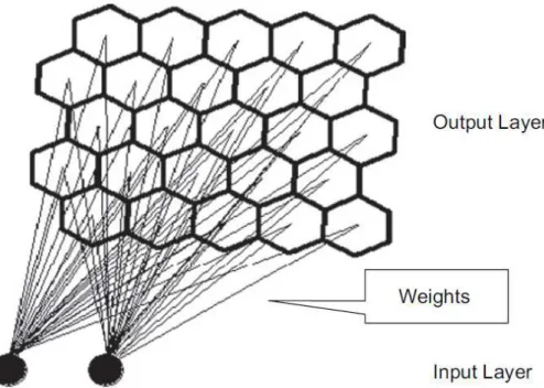
tion purposes) discrete lattice of neurons in an output layer (Kohonen, 2001; Kalteh, 2008).

Typically a SOM consists of two layers, an input layer and a Kohonen or output layer (see Fig. 1 after Kalteh et al., 2008). The input layer contains one neuron for each variable (i.e., catchment attribute) in the data set. The number of classes (i.e.,

15

neurons of the output layer) is generally predefined by the modeller and the classes themselves are ordered into meaningful maps that preserve the topology (see Kalteh et al., 2008). The output-layer neurons are connected to every neuron in the input layer through adjustable weights (see Fig. 1), whose values are identified through an iterative training procedure. Following a random initialisation of the weight vectors , SOM utilizes

20

a type of learning that is called competitive, unsupervised, or self-organizing procedure to match each input vector with only one neuron in the output layer. This is done by comparing the presented input pattern with each of the SOM neuron weight vectors, on the basis of a distance measure, like the Euclidean distance. The neuron with the closest match to the presented input pattern is called winner neuron. Then, the weight

25

(7)

HESSD

8, 391–427, 2011

Title Page

Tables Figures

◭ ◮

Back Close

Full Screen / Esc

Discussion

P

a

per

|

Dis

cussion

P

a

per

|

Discussion

P

a

per

|

Discussio

n

P

a

per

|

Once trained (calibrated), the network activates only one output node in correspon-dence of each input vector. Therefore, all input vectors activating the same node belong to the same class.

3 Multivariate analysis for dimensionality reduction

3.1 Principal component analysis – PCA

5

The Principal Component Analysis, PCA, PCA (see e.g., Krzanowski, 1988) is a multi-variate analysis statistical method that enables one to obtain smaller number of uncor-related variables from a larger number of possibly coruncor-related variables by constructing an orthogonal basis for the original variables themselves. The derived uncorrelated variables are called principal components (PC). The full set of PC’s has the same

di-10

mensionality of the original set of variables. They are ordered in such a way that the first component accounts for as much of the variability in the original dataset as possible, and each following PC accounts for as much of the remaining variability as possible.

It is commonplace for the sum of the variances of the first few PCs to exceed 80% of the total variance of the original data. By examining plots of these few new variables,

15

researchers often develop a deeper understanding of the driving forces that generated the original data. The literature reports several criteria for selecting the appropriate number of principal components (see e.g., Kaiser, 1960 criterion and the scree plot). 3.2 Canonical correlation analysis – CCA

Another important multivariate statistical tool for reducing the dimensionality of the

orig-20

(8)

HESSD

8, 391–427, 2011

Title Page

Tables Figures

◭ ◮

Back Close

Full Screen / Esc

Discussion

P

a

per

|

Dis

cussion

P

a

per

|

Discussion

P

a

per

|

Discussio

n

P

a

per

|

as the annual flow, the flood associated with a given recurrence interval, etc.). CCA enables one to identify the dominant linear modes of covariability between the setsX andY _{(see e.g., Krzanowski, 1988; Ouarda et al., 2001). In other words, CCA} iden-tifies two new groups of artificial variables (canonical variables)U=_{_U₁_,_U₂_,...,_U_r_}_and V=_{_V₁_,_V₂_,...,_V_r_}_{, with}_r=_min_{_n_,_m_}_{, by finding linear combinations of the original}_X_i_{, with}

5

i=_1,...,_n_{, and}_Y_j_{, with}_j=_1,...,_m_{, in such a way that the correlation between the} canoni-cal variables of a pair (U_i,V_i) is maximized and the correlation between the variables of diff_{erent pairs is null (Chokmani and Ouarda, 2004; Shu and Ouarda, 2007).}

If we denote byX _andY _{the independent and dependent variables respectively and} we consider the linear transformations,

10

U=uT

X·X andV=u

T

Y·Y (1)

characterized by the basis vectorsu_X _and u_Y_{, CCA can be defined as the following} optimization problem,

ρ= _max

u_X,v_Y{corr(U,V)}=umax_X,v_Y

cov(U_,V₎

p

var(U₎p_var(V₎

. (2)

4 Study area and available information

15

The study area consists of the entire Italian peninsula and it is definitely heteroge-neous in terms of climatic and geomorphologic characteristics that control the stream-flow regime. In particular, the study focuses on 296 Italian catchments scattered na-tionwide, whose dataset was compiled within the national research project “CUBIST – Characterisation of Ungauged Basins by Integrated uSe of hydrological Techniques”

20

(9)

HESSD

8, 391–427, 2011

Title Page

Tables Figures

◭ ◮

Back Close

Full Screen / Esc

Discussion

P

a

per

|

Dis

cussion

P

a

per

|

Discussion

P

a

per

|

Discussio

n

P

a

per

|

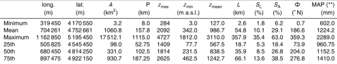
4.1 Geomorphoclimatic and streamflow variables

We refer to 12 diff_{erent geomorphological and climatic descriptors of the study} catch-ments, which we term in the studyX variables, and 6 descriptors of the streamflow regime, which we termY variables.

5

X variables:

– (1 and 2) long. and lat. – UTM longitude and latitude of catchment centroid; – (3)A– Drainage area;

– (4)P – Perimeter;

– (5)zmax– Highest elevation; 10

– (6)zmin– Elevation of the catchment outlet;

– (7)zmean– Mean altitude;

– (8)L– Maximum drainage length;

– (9)SL– Average slope along the Maximum drainage length;

– (10)SA– Catchment average slope; 15

– (11)Φ_{– Catchment orientation;}

– (12) MAP – Mean Annual Precipitation;

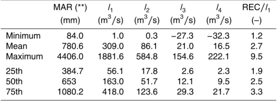
Y variables:

– (1) MAR – Mean Annual Runoff_;

– (from 2 to 5)l_i – sample L moments of order i=_{1 (i.e. sample mean), 2, 3 and 4}

20

(10)

HESSD

8, 391–427, 2011

Title Page

Tables Figures

◭ ◮

Back Close

Full Screen / Esc

Discussion

P

a

per

|

Dis

cussion

P

a

per

|

Discussion

P

a

per

|

Discussio

n

P

a

per

|

– (6) REC/l1– Ratio between the maximum value and the sample mean of AMS of

flood flows.

Tables 1 and 2 summariseX andY variables in terms of minimum, mean and maximum values, and 25th, 50th and 75th percentiles for the set of 296 considered catchments. 4.2 Application of PCA and CCA

5

We reduced the dimensionality of the 12-dimensional space of the geomorphoclimatic descriptors (X variables) and the 6-dimensional space of the streamflow regime de-scriptors (Y variables) through the application of PCA and CCA. In particular we com-puted all PC’s of X variables relative to the whole set of 296 basins. As said before, the full set of PC’s is as large as the original set of variables. The 12 PC’s have zero mean

10

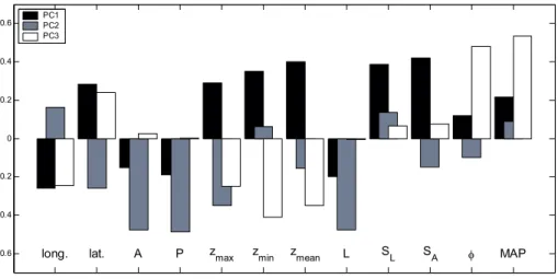
and a decreasing standard deviation (see Table 3), but the most interesting property is that the first three principal components explain roughly the two third of the total variability, in this case more than the 75.4% (Table 3).

Figure 2 reports the coeffi_{cients of linear transformation of each} _X _{variable for the} first three Principal Components. This information is explained from the eigenvalues

15

calculated for our dataset.

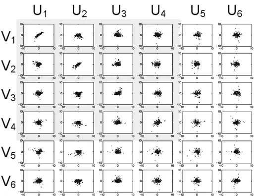
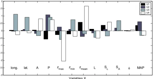
Likewise, we applied the CCA to the set ofX andY variables relative to the whole of the 296 study basins. As reported above, the number of canonical variables is equal to the smallest minimum dimension of the two sets of variables, in our case the Y

variables. Therefore we obtained 6 canonical variables for each set,U _andV_.

20

The scatter-plots of Fig. 3 illustrate the relationships between the canonical variables U ₍_x _{axis) and} V ₍_y _{axis) computed for the study area, also illustrating, as expected,} a significant correlation between the first canonical variablesU_i andV_i. Table 4 shows the significance of the null hypothesis that all correlation coeffi_{cients between}_U_j _and_V_j_, withj=_i_{, ...,}_r=_{6, are all zero. As Table 4 shows, the first 4 canonical variables are the}

25

(11)

HESSD

8, 391–427, 2011

Title Page

Tables Figures

◭ ◮

Back Close

Full Screen / Esc

Discussion

P

a

per

|

Dis

cussion

P

a

per

|

Discussion

P

a

per

|

Discussio

n

P

a

per

|

5 Comparison of SOM classifications of the study catchments

5.1 Reference and alternative SOM classifications

There are no predefined classes of the conditions characterising the basin: a clustering algorithm is here used as an unsupervised classifier, where the task is to learn a clas-sification from the data. Such partitioning will be based on the most relevant available

5

information, that is, descriptors of the streamflow regime and geomorphoclimatic char-acteristics.

We considered 5 diff_{erent SOM classifications: a reference SOM classification and 4} alternative SOM classifications. These classifications were obtained for the considered group of catchments on the basis of the information described below:

10

– Reference Classification (RC)

– SOMY is obtained by using indices of the streamflow regime (Y variables); – Alternative Classifications (ACs):

– SOMX is based upon the geomorphoclimatic descriptors (X variables); – SOMPC3 uses the first three Principal Components of theX variables;

15

– SOMU uses all canonical variables computed by applying CCA to X and Y

variables (i.e.,U_i, withi=_{1, ..., 6);}

– SOMU4 uses a subset containing the most descriptive canonical variables (i.e.,Ui, withi=1, ..., 4).

5.2 SOM classification implementation

20

(12)

HESSD

8, 391–427, 2011

Title Page

Tables Figures

◭ ◮

Back Close

Full Screen / Esc

Discussion

P

a

per

|

Dis

cussion

P

a

per

|

Discussion

P

a

per

|

Discussio

n

P

a

per

|

it was here chosen an hexagonal topology formed by three rows by three columns, for a total of nine nodes, each one corresponding to a class, believing that such number is adequate for representing a variety of homogeneous, but suffi_{ciently numerous, groups} of watersheds.

We used the Euclidean distance as a measure of the distance between the vectors,

5

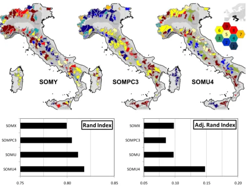
according to the majority of hydrological applications. Three out of five SOM’s classifi-cations resulting from the diff_{erent sets of descriptors are represented in Fig. 5 (SOMX} and SOMU were omitted due to space limitations). Note that no relationship exists between classes depicted by the same colour in diff_{erent classifications.}

It is worth noting here that RC is identified on the basis of indices characterizing

10

the streamflow regime, whereas all AC’s are delineated by applying SOM techniques to information that can be retrieved for ungauged basins. Any ungauged basin, once characterized in terms of the 12 considered catchment descriptors, can be allocated to one of the nine classes of each alternative SOM classifications. The regional stream-flow information collected within the class to which the ungauged site belongs can then

15

be used to infer the streamflow regime of the ungauged site itself.

The next two sections assess the eff_{ectiveness of AC’s in terms of (1) a}ffi_{nity to the} RC and (2) usability in the PUB context to predict the streamflow regime in ungauged catchment.

5.3 Affinities of alternative SOM classifications with the reference classification

20

Two indices of similarity were applied to quantify the affi_{nities between reference} (SOMY) and alternative classifications: the Rand Index (Rand, 1971), RI, and its vari-ation proposed by Hubert and Arabie (1985).

Comparing two partitions (P1andP2) of the same data set, a couple of objects (i.e.,

catchments) can belong to the same class or diff_{erent classes in} _P₁ _and _P₂_{. Let us}

25

(13)

HESSD

8, 391–427, 2011

Title Page

Tables Figures

◭ ◮

Back Close

Full Screen / Esc

Discussion

P

a

per

|

Dis

cussion

P

a

per

|

Discussion

P

a

per

|

Discussio

n

P

a

per

|

as the number of catchments that belong to diff_{erent classes both in}_P₁_and_P₂_{. Under} these assumptions, RI reads,

RI= N11+N00

N11+N00+N10+N01

(3)

RI varies between 1 (perfect agreement between the two partitions) and 0 (no agree-ment).

5

Hubert and Arabie (1985) proposed an adjustment to the Rand Index so that its ex-pected value is equal to zero for random partitions having the same number of objects in each class. The index is still equal to 1 for perfect agreement but it can also take negative values (higher discriminatory power than RI).

The bar-diagram of Fig. 5 shows the values obtained for these indices by comparing

10

the RC (i.e., SOMY) with all AC’s (i.e., SOMX, SOMPC3, SOMU and SOMU4). RC is based on the use of hydrometric information, therefore the eff_{ectiveness of all AC’s,} which are suitable for ungauged basins, is “measured” relative to SOMY.

Figure 5 shows that, as it was expected, SOMX and SOMPC3 are similar to each other in terms of affi_{nity with SOMY. Figure 5 also shows that SOMU and SOMU4 are}

15

more similar to SOMY than SOMX and SOMPC3, indicating that SOMU4 outperforms all other classifications in terms of affi_{nity with the reference classification SOMY.}

These results are a consequence of the intrinsic nature of the alternative SOM clas-sifications considered in our study. SOMX uses all geomorphological and climatic de-scriptors, therefore there is no direct relationship with the information used for

delin-20

eating SOMY and, also, the information utilised to delineate SOMX presents redun-dancy that may impact the effi_{ciency of the classification process. SOMPC3 uses} only the most descriptive portion of the available geomorphologic and climatic infor-mation, therefore removing some noise from the input data, yet no direct relation with the hydrometric information also in this case. SOMU, instead, uses as input

informa-25

(14)

HESSD

8, 391–427, 2011

Title Page

Tables Figures

◭ ◮

Back Close

Full Screen / Esc

Discussion

P

a

per

|

Dis

cussion

P

a

per

|

Discussion

P

a

per

|

Discussio

n

P

a

per

|

5.4 Quantitative comparison of SOM classifications in the PUB context

The eff_{ectiveness of each classification has been further assessed relative to the} esti-mation of streamflow regime for ungauged sites. To this aim we developed a number of multiple regression models for estimating the streamflow index of interest in ungauged sites and we assessed the performances of these models in cross-validation for all AC’s

5

considered in the study, to better understand whether or not the utilization of PCA and CCA may improve the practical usability of SOM catchment classifications, reducing the uncertainty of predictions in ungauged sites.

For the sake of generality and simplicity, we referred in the study to the simplest possible model structure, therefore adopting a linear multiregression model as the

ref-10

erence model. The model reads, ˆ

yi=A0+A1PC1i+A2PC2i+A3PC3i+ϑ (4a)

whereA0,A1, andA3 are the parameters of the multivariate linear regression model;

PC1_i, PC2_i and PC3_i are the first three principal components of variablesX for site

i, withi=_{1, ..., 296, which explain more than the 75.4% of the total variance and, for}

15

consistency, are used as explanatory variables in all multiregression models developed in the study;ϑis the residual of the model; and ˆyi is the normalized streamflow index

of interest for sitei,

ˆ

y_i=zˆi−z¯

s_Z , (4b)

with ˆzi empirical value of the streamflow index for sitei, and ¯z andsZ empirical mean

20

and standard deviation of the streamflow index of interest for the entire dataset. We performed this analysis by developing for each catchment classification of in-terest four diff_{erent multiregression models (Eq. 4a), namely one model for estimating} of Mean Annual Runoff _{(MAR) and three models for estimating the first 3 sample L} moments of the annual maximum seriesl1,l2 and l3. In particular, four models were 25

(15)

HESSD

8, 391–427, 2011

Title Page

Tables Figures

◭ ◮

Back Close

Full Screen / Esc

Discussion

P

a

per

|

Dis

cussion

P

a

per

|

Discussion

P

a

per

|

Discussio

n

P

a

per

|

of the four AC’s (i.e., SOMX, SOMPC3, SOMU and SOMU4). Four multiple linear re-gression models were also identified for the entire national set of basins (NOCLASS), which represents a baseline condition in the comparison and sets the minimum level of performance.

We assessed the effi_{ciency of each alternative classification AC by referring to the}

5

results of an extensive jack-knife cross-validation of all 24 regression models developed for the six identified classifications (i.e., RC -optimal-, AC’s, NOCLASS -baseline-).

The jack-knife cross-validation procedure is applied in order to quantify the accuracy of each model when applied in ungauged basins; it is also called in the literature as delete-one or leave-one-out cross-validation procedure (see e.g., Efron, 1982; Zhang

10

and Kroll, 2007; Brath et al., 2003; Castellarin et al., 2004). This method is extremely versatile and capable of providing adequate evaluation of the performance of the in-terpolation techniques, since it simulates the ungauged conditions for each site in the study region. The procedure can be illustrated as follows,

(a) one catchment is eliminated from the set ofN catchments;

15

(b) an empirical multiregression model is identified on the basis of the information col-lected at theN−1 remaining catchments (i.e., the first three principal components are computed and the coeffi_cients_A_j _{of Eq. (4a), with} _j=_{0, ..., 3, are estimated} through linear multiregression techniques);

(c) the model developed at step (b) is used for estimating the streamflow index at the

20

discarded site;

(d) steps (a) to (c) are repeatedN−1 times, each time by eliminating a diff_erent catch-ment.

In a few words, the jack-knife procedure estimates the streamflow index at stake in a given site without taking into account the hydrometric information available at the site

25

(16)

HESSD

8, 391–427, 2011

Title Page

Tables Figures

◭ ◮

Back Close

Full Screen / Esc

Discussion

P

a

per

|

Dis

cussion

P

a

per

|

Discussion

P

a

per

|

Discussio

n

P

a

per

|

The results of the various cross-validations were quantified in terms of Nash-Sutcliff_e effi_{ciency measure (NSE) (Nash and Sutcli}ff_{e, 1970). The NSE varies in the range} ]−∞, 1], where 1 corresponds to a perfect agreement between modelled and empirical values, NSE=_{0 indicates that estimated values are as accurate as the mean of the} ob-served values, while negative values occur when the obob-served mean value is a better

5

predictor than the model. The performance index reads

NSE=₁₋

P

i=1,N

ηJK,i−ηi

2

P

i=1,N

η_i− P

i=1,N

_η

i

N

!2 (5)

whereηJK,i indicates the jack-knife estimate andηi the empirical value for sitei, with

i=_{1, ...,}_N_.

We computed the performance index relative to jack-knife and empirical values of

10

MAR (Mean Annual Runoff_{) and}_l₁_{(mean annual flood). Producing reliable predictions} of MAR andl1 in ungauged sites is of primary concern (see e.g., Brath et al., 2001;

Castellarin et al., 2004; Kjeldsen and Jones, 2010). Concerning the higher order L mo-ments (i.e.,l2andl3), instead of comparing directly empirical and jack-knife values we

preferred to focus on flood quantiles (i.e. flood flows associated with a given recurrence

15

intervalT), computed on the basis of the L-moments. We deem the flood quantiles to be more meaningful and understandable thanl2and l3 for summarising the flood

fre-quency regime from a practical viewpoint. Ultimately, hydrologists and practitioners are interested in the estimation of the design flood in ungauged sites rather than the L moments’ values.

20

We estimated the flood quantiles at each and every site from a Generalized Extreme-Value (GEV) estimated with the L moments method (GEV-LMOM algorithm), which is often more effi_{cient than the maximum likelihood when used with small to moderate} length samples (please refer to Hosking and Wallis, 1997 for details of the frequency distribution and the method of L moments). The GEV distribution was selected in light

(17)

HESSD

8, 391–427, 2011

Title Page

Tables Figures

◭ ◮

Back Close

Full Screen / Esc

Discussion

P

a

per

|

Dis

cussion

P

a

per

|

Discussion

P

a

per

|

Discussio

n

P

a

per

|

of its satisfactorily reproduction of the sample frequency distribution of hydrological extremes in Italy and around the world (see e.g., Stedinger et al., 1993; Robson and Reed, 1999; Castellarin et al., 2001).

We arbitrarily selected three diff_{erent return periods,} _T=_{10, 50 and 100 years and} we estimated the flood quantiles through the GEV-LMOM algorithm by referring to the

5

sample L momentsl1,l2 andl3 and their jack-knife estimates for all classifications of

interest (RC, AC’s, NOCLASS). We then compared these estimates in terms of Eq. (5). To avoid unduly extrapolations, we limited the comparison forT=_{10 and 50 years to} the 92 out of 296 sites with at least 30 years of observed annual maxima, and to the 34 out of 296 sites with at least 40 years of observations forT=_{50 and 100 years.}

10

It is worth highlighting here that even though the use of NSE has become a natural part of the modelling practice, its utilization is still a matter of concern (see e.g., Gupta et al., 2009). In fact, the usefulness of the observed mean as a reference value varies strongly in practical applications. Like all the squared measures, NSE weights the largest observation very heavily at the expense of smaller values, to overcome this

15

problem we performed the NSE on logflows, this is typically considered valuable for flood and mean annual streamflows.

6 Results and discussion

Table 5 reports the values obtained for NSE for all cross-validated streamflow indices and classifications. The scatter plots of Fig. 6 report sample estimates of streamflow

20

indices of interest against predicted values obtained in cross-validation for some of the classifications considered in the study. Distribution of relative residuals between empirical and jack-knifed values of the streamflow index of interest are illustrated in Fig. 7 for NOCLASS, SOMY, SOMPC3 and SOMU.

The comparison between the results obtained for the baseline condition (NOCLASS)

25

(18)

HESSD

8, 391–427, 2011

Title Page

Tables Figures

◭ ◮

Back Close

Full Screen / Esc

Discussion

P

a

per

|

Dis

cussion

P

a

per

|

Discussion

P

a

per

|

Discussio

n

P

a

per

|

considered multiregressive model for all streamflow indices considered in the study. NSE values show significant improvements for all streamflow indices and alternative classifications relative to NOCLASS (see Table 5). Also, the comparison between the results obtained for SOMX and those relative to SOMPC3, SOMU and SOMU4 points out that combining SOM with PCA or CCA can improve eff_{ectiveness and usefulness}

5

of SOM classifications in the PUB context, that is for predictions of streamflow indices in ungauged basins.

Results reported in Table 5 indicate that multiregression models based on SOMU4 outperform the other models for predicting MAR in ungauged basins. SOMU4 is as accurate as the optimal classification SOMY in predicting MAR in ungauged basins.

10

Table 5 illustrates a diff_{erent picture for the prediction of the annual flood (}_l₁_{). In this} case the application of SOMPC3 results in the best NSE value, but, above all, perfor-mances of all alternative classifications are similar and low, definitely lower than SOMY and comparable with NOCLASS performances. This result was somehow expected, ours study adopts a very simplistic model (see Eq. 4) and the prediction of the central

15

tendency of the flood frequency distribution (e.g., annual flood, median, index-flood, etc.) is indicated by the literature as one of the most critical steps required by the ap-plication of regional models to ungauged sites and is generally associated with a large uncertainty (see e.g., Brath et al., 2001; Castellarin, 2007; Kjeldsen and Jones, 2010). Concerning the prediction of flood quantiles, the results of our study point out a clear

20

supremacy of SOMU. Table 5 indicates that SOMU is associated with the highest NSE values 3 out of 4 times. It is interesting to note that also SOMPC3 shows good perfor-mances, implying that the removal of redundant information involved in the identifica-tion of SOMX improves the accuracy of the regional models. Nevertheless, the lower bias and variability of residuals of SOMU relative to SOMPC3 is also evident in the

25

boxplots of Fig. 7.

(19)

HESSD

8, 391–427, 2011

Title Page

Tables Figures

◭ ◮

Back Close

Full Screen / Esc

Discussion

P

a

per

|

Dis

cussion

P

a

per

|

Discussion

P

a

per

|

Discussio

n

P

a

per

|

and upper quartiles which is 1.5 times larger than the distance between the quartiles themselves). This may be due to the extreme simplicity of the linear regional model and the huge variability of climatic and hydrological characteristics of the consider catch-ments.

Furthermore, results obtained for SOMY (reference classification) and SOMX,

5

SOMPC3, SOMU4 and SOMU reported in Table 5 and Fig. 7 also point out rather clearly that, aside from predictions of MAR, there is still a great margin for improve-ments. The gap in terms of performance between regional models based on SOMY and models based on all alternative classifications is significant. It is worth noting that this outcome has nothing to do with the limitations of the simplistic regional model

10

adopted in the study (i.e., Eq. 4), nor the information used by the regional model. The structure of the regional model does not vary and the predictions in cross-validation of all regional model are based upon the same information (i.e., first three principal components ofX variables). Simply, SOMY transfers the streamflow information from gauged sites to ungauged ones in a more eff_{ective way. None of the catchment}

classi-15

fications based directly (SOMX) or indirectly (SOMPC3, SOMU, SOMU4), on the avail-able catchment descriptors is as effi_{cient as SOMY in transferring the streamflow} infor-mation form gauged to ungauged sites. This gap may be reduced by identifying more informative catchment descriptors (see e.g., Savenije, 2010) given the growing avail-ability of easily accessible high resolution topographic and land-cover data, together

20

with GIS tools for hydrologic analysis. Further improvements may probably stem from a process-based reorganization of the available information based on physically-based criteria that aims at further removing some noise characterizing the available set of catchment descriptors.

Future analyses, possibly focussing on larger datasets and diverse climatic and

25

(20)

HESSD

8, 391–427, 2011

Title Page

Tables Figures

◭ ◮

Back Close

Full Screen / Esc

Discussion

P

a

per

|

Dis

cussion

P

a

per

|

Discussion

P

a

per

|

Discussio

n

P

a

per

|

of concentration or drainage density (Pallard et al., 2009), and (2) raw climatic informa-tion (e.g., catchment scale mean monthly and annual precipitainforma-tion and temperature) to estimate aridity indices or net precipitation (Castellarin et al., 2007).

7 Conclusions

Our study analyses the eff_{ectiveness of unsupervised neural networks (Self Organising}

5

Maps, SOM) coupled with multivariate techniques for reducing the high dimensional-ity of catchment descriptors (i.e., Principal Component Analysis, PCA, and Canonical Correlation Analysis CCA) for producing catchment classifications on objective bases. Catchment classification does not have a purpose in itself in the context of our anal-ysis, and does not represent a mere scientific exercise, but represents the means to

10

transfer information from gauged sites to ungauged ones, reducing the uncertainty of hydrological predictions in ungauged sites.

We consider some 300 Italian catchments scattered nationwide, which represent a complex compound featuring all Italian hydro-climatic settings, from Alpine to Mediter-ranean, from humid to semiarid, and from continental to maritime conditions.

15

The catchments are grouped into five diff_{erent classifications, all delineated by} means of unsupervised neural networks. One reference classification is identified by using as catchment descriptors indices of the streamflow regime and flood statistics (reference classification). Four alternative classifications are derived by referring to a number of geomorphologic and climatic catchment descriptors which can be

com-20

puted for ungauged basins. One of this classification uses the entire set of descriptors as input variables to SOM, whereas the remaining three alternative classifications uti-lize as input variables a limited number of measures that are linear combinations of the original catchment descriptors obtained by applying PCA or CCA.

We compared the similarity of the alternative classifications with the reference

clas-25

(21)

HESSD

8, 391–427, 2011

Title Page

Tables Figures

◭ ◮

Back Close

Full Screen / Esc

Discussion

P

a

per

|

Dis

cussion

P

a

per

|

Discussion

P

a

per

|

Discussio

n

P

a

per

|

on the alternative catchment classifications with the accuracy of the same predictions based on (1) the reference classification and (2) a baseline condition which groups together the entire system of Italian catchments (absence of classification). The re-gional predictions are obtained through the application of an extensive cross-validation procedure that simulates the ungauged conditions at each and every site.

5

Main outcomes of the study may be summarised as follows: (i) SOM’s confirm their eff_{ectiveness and usefulness as objective criteria for pattern recognition and, in} par-ticular, for delineating catchment classifications; (ii) PCA and CCA can significantly improve the eff_{ectiveness and usefulness of SOM in the context of PUB, that is for} reducing the uncertainty of hydrological predictions in ungauged sites; we strongly

en-10

courage to perform PCA, and in particular CCA, on the available set of catchment descriptors before applying SOM; (iii) catchment classification provides a great deal of information for enhancing hydrological predictions in ungauged basins, yet the applica-tion of objective but merely statistical criteria and algorithms (PCA and CCA with SOM) revealed some limitations that may be significantly reduced by switching from

data-15

driven to data- and process-driven catchment classification. Designing a theoretical framework for combining these two diff_{erent perspectives is an exciting open problem} for future analyses.

Acknowledgement. The study has been partially supported by the Italian Government through its national grants to the programmes on “Advanced techniques for estimating the magnitude

20

and forecasting extreme hydrological events, with uncertainty analysis” and “Relations between hydrological processes, climate, and physical attributes of the landscape at the regional and basin scales”.

References

Acreman, M. C. and Sinclair, C. D.: Classification of drainage basins according to their physical

25

(22)

HESSD

8, 391–427, 2011

Title Page

Tables Figures

◭ ◮

Back Close

Full Screen / Esc

Discussion

P

a

per

|

Dis

cussion

P

a

per

|

Discussion

P

a

per

|

Discussio

n

P

a

per

|

Bai, Y., Wagener, T., and Reed, P.: A top-down framework for watershed model evaluation and selection under uncertainty, Environ. Model. Softw., 24(8), 901–916, doi:10.1016/j.envsoft.2008.12.012, 2009.

Brath, A., Castellarin, A., Franchini, M., and Galeati, G.: Estimating the index flood using indi-rect methods, Hydrol. Sci. J., 46(3), 399-418, 2001.

5

Brath, A., Castellarin, A., and Montanari, A.: Assessing the reliability of regional depth-duration-frequency equations for gauged and ungauged sites, Water Resour. Res., 39(12), 1367, doi:10.1029/2003WR002399, 2003.

Burn, D. H.: Cluster analysis as applied to regional flood frequency, J. Water Res. Pl.-ASCE, 115(5), 567–582, 1989.

10

Castellarin, A.: Application of probabilistic envelope curves for design-flood estimation at un-gaged sites, Water Resour. Res., 43, W04406, doi:10.1029/2005WR004384, 2007.

Castellarin, A., Burn, D. H., and Brath, A.: Assessing the effectiveness of hydrological similarity measures for regional flood frequency analysis, J. Hydrol., 241(3–4), 270–285, 2001. Castellarin, A., Galeati, G., Brandimarte, L., Brath, A., and Montanari, A.: Regional

flow-15

duration curve: realiability for ungauged basins, Adv. Water Resour., 27(10), 953–965, 2004. C ´er ´eghino, R. and Park, Y. S.: Review of the self-organizing map (SOM) approach in water

resources: commentary, Environ. Model. Softw., 24(8), 945–947, 2009.

Chokmani, K. and Ouarda, T. B. M. J.: Physiographical space-based kriging for regional flood frequency estimation at ungauged sites, Water Resour. Res., 40(12), W12514,

20

doi:10.1029/2003WR002983, 2004.

Claps, P., Barberis, C., De Agostino, M., Gallo, E., Laio, F., Miotto, F., Plebani, F., Vezz `u, G., Zanetta, M., Laguardia, G., and Viglione, A.: Development of an information system of the Italian basins for the CUBIST project, Geophys. Res. Abstr., (ISSN 1029-7006), Vol. 10, EGU2008-A-12048, SRef-ID: 1607-7962/gra/EGU2008-A-12048, 2008.

25

Dawson, C. W. and Wilby, R. L.: Hydrological modelling using artificial neural networks, Progress Phys. Geogr., 25(1), 80–108, 2001.

Dooge, J. C. I.: Looking for hydrologic laws, Water Resour. Res., 22(9), 46–58, 1986.

Efron, B.: The Jackknife the Bootstrap and Other Resampling Plans, Society for Industrial and Applied Mathematics, Philadelphia, Pennsylvania, 1982.

30

(23)

HESSD

8, 391–427, 2011

Title Page

Tables Figures

◭ ◮

Back Close

Full Screen / Esc

Discussion

P

a

per

|

Dis

cussion

P

a

per

|

Discussion

P

a

per

|

Discussio

n

P

a

per

|

Hall, M. J. and Minns, A. W.: The classification of hydrologically homogeneous regions, Hydrol. Sci. J., 44(5), 693–704, 1999.

Hosking, J. R. M.: L-moments: analysis and estimation of distributions using linear combina-tions of order statistics, J. R. Stat. Soc. B, 52, 105–124, 1990.

Hosking, J. R. M. and Wallis, J. R.: Regional Frequency Analysis, Cambridge University Press,

5

Cambridge, 1997.

Hubert, L. and Arabie, P.: Comparing partitions, J. Classif., 2, 193–218, 1985.

Jingyi, Z. and Hall, M. J.: Regional flood frequency analysis for the Gan-Ming River basin in China, J. Hydrol., 296, 98–117, 2004.

Kaiser, H. F.: The application of electronic computers to factor analysis, Educ. Phychol. Meas.,

10

20, 141–151, 1960.

Kalteh, A. M., Hjorth, P., and Berndtsson, R.: Review of the self-organizing map (SOM) ap-proach in water resources: analysis, modelling and application, Environm. Model. Softw., 23, 835–845, 2008.

Kjeldsen, T. R. and Jones, D. A.: Predicting the index flood in ungauged UK catchments: on

15

the link between data-transfer and spatial model error structure, J. Hydrol., 387(1–2), 1–9, 2010.

Kohonen, T.: Self-organized formation of topologically correct feature maps, Biol. Cybern., 43, 59–69, 1982.

Kohonen, T.: Self-Organizing Maps, 2nd ed., Springer, Berlin, 1997.

20

Krzanowski, W. J.: Principles of Multivariate Analysis, Oxford University Press, Oxford, 1988. McDonnell, J. J., Sivapalan, M., Vach ´e, K., Dunn, S., Grant, G., Haggerty, R., Hinz, C., Hooper,

R., Kirchner, J., Roderick, M. L., Selker, J., and Weiler, M.: Moving beyond heterogeneity and process complexity: lA new vision for watershed hydrology, Water Resour. Res., 43, W07301, doi:10.1029/2006WR005467, 2007.

25

McDonnell, J. J. and Woods, R. A.: On the need for catchment classification, J. Hydrol., 299, 2–3, 2004.

Maier, H. R. and Dandy, G. C.: Neural networks for the prediction and forecasting of water resources variables: a review of modelling issues and applications, Environ. Model. Softw., 15, 101–123, 2000.

30

(24)

HESSD

8, 391–427, 2011

Title Page

Tables Figures

◭ ◮

Back Close

Full Screen / Esc

Discussion

P

a

per

|

Dis

cussion

P

a

per

|

Discussion

P

a

per

|

Discussio

n

P

a

per

|

Nash, J. and Sutcliffe, J.: River flow forecasting through conceptual models, Part 1: a discussion of principles, J. Hydrol., 10, 282–290, 1970.

Ouarda, T., Girard, C., Cavadias, G. S., and Bob ´ee, B.: Regional flood frequency estimation with canonical correlation analysis, J. Hydrol., 254, 157–173, 2001.

Pallard, B., Castellarin, A., and Montanari, A.: A look at the links between drainage density and

5

flood statistics, Hydrol. Earth Syst. Sci., 13, 1019–1029, doi:10.5194/hess-13-1019-2009, 2009.

Rand, W. M.: Objective criteria for the evaluation of clustering methods, J. Am. Stat. Assoc., 66(336), 846–850, doi:10.2307/228423, 1971.

Robson, A. J. and Reed, D. W.: Statistical procedures for flood frequency estimation, Vol. 3 in:

10

Flood Estimation Handbook (FEH), Institute of Hydrology, Wallingford (UK), 1999.

Savenije, H. H. G.: HESS Opinions “Topography driven conceptual modelling (FLEX-Topo)”, Hydrol. Earth Syst. Sci., 14, 2681–2692, doi:10.5194/hess-14-2681-2010, 2010.

Shu, C. and Ouarda, T. B. M. J.: Flood frequency analysis at ungauged sites using artificial neural networks in canonical correlation analysis physiographic space, Water Resour. Res.,

15

15(43), W07438, doi:10.1029/2006WR005142, 2007.

Sivapalan, M., Takeuchi, K., Franks, S. W., Gupta, V. K., Karambiri, H., Lakshmi, V., Liang, X., Mcdonnell, J. J., Mendiondo, E. M., O’connell, P. E., Oki, T., Pomeroy, J. W., Schertzer, D., Uhlenbrook, S., and Zehe, E.: IAHS decade on predictions in ungauged basins (PUB), 2003–2012: shaping an exciting future for the hydrological sciences, Hydrol. Sci. J., 48(6),

20

857–880, 2003.

Srinivas, V. V., Tripathi, S., Rao, A. R., and Govindaraju, R. S.: Regional flood frequency anal-ysis by combining self-organizing feature map and fuzzy clustering, J. Hydrol., 348(1–2), 148–166, 2008.

Stedinger, J. R., Vogel, R. M., and Foufoula-Georgiou, E.: Frequency analysis of extreme

25

events, Chapt. 18, in: Handbook of Hydrology, edited by: Maidment, D. R., McGraw-Hill Inc., New York (NY, USA), 1993.

Toth, E.: Classification of hydro-meteorological conditions and multiple artificial neural networks for streamflow forecasting, Hydrol. Earth Syst. Sci., 13, 1555–1566, doi:10.5194/hess-13-1555-2009, 2009.

30

Vesanto, J.: SOM-based data visualization methods, Intell. Data Anal., 3, 111–126, 1999. Wagener, T., Sivapalan, M., Troch, P., and Woods, R.: Catchment classification and hydrologic

(25)

HESSD

8, 391–427, 2011

Title Page

Tables Figures

◭ ◮

Back Close

Full Screen / Esc

Discussion

P

a

per

|

Dis

cussion

P

a

per

|

Discussion

P

a

per

|

Discussio

n

P

a

per

|

Yan, X., Chen, D., Chen, Y., and Hu, S.: SOM integrated with CCA for the feature map and classification of complex chemical patterns, Comput. Chem., 25(6), 597–605, 2001.

(26)

HESSD

8, 391–427, 2011

Title Page

Tables Figures

◭ ◮

Back Close

Full Screen / Esc

Discussion

P

a

per

|

Dis

cussion

P

a

per

|

Discussion

P

a

per

|

Discussio

n

P

a

per

|

Table 1. Minimum, mean and maximum values, and 25th, 50th and 75th percentiles for the set ofX variables considered in the study. These data were either derived from a SAR-DTM (Synthetic Aperture Radar-Digital Terrain Model) with grid size 100 m or (**) retrieved from Rep. no. 17 of the former Italian SIMN (National Hydrographic Service of Italy.

long. lat. A P zmax zmin zmean L SL SA Φ MAP (**)

(m) (m) (km2) (km) (m a.s.l.) (km) (%) (%) (◦N) (mm)

Minimum 319 450 4 170 550 3.2 8.0 284 3.0 127.0 2.6 1.8 6.2 0.7 602.0

Mean 704 261 4 752 661 1060.8 157.8 2092 342.0 986.7 54.8 10.1 29.1 186.6 1224.2

Maximum 1 162 850 5 195 450 17 512.1 1115.0 4727 1812.0 3110.0 357.9 35.4 63.0 359.3 2289.0

25th 505 825 4 545 450 98.0 52.75 1409 77.7 567.5 18.7 5.3 18.4 73.9 960.75

50th 680 450 4 814 250 331.0 102.5 1814 231.5 838.5 35.9 8.5 26.8 204.0 1152.5

(27)

HESSD

8, 391–427, 2011

Title Page

Tables Figures

◭ ◮

Back Close

Full Screen / Esc

Discussion

P

a

per

|

Dis

cussion

P

a

per

|

Discussion

P

a

per

|

Discussio

n

P

a

per

|

Table 2. Minimum, mean and maximum values, and 25th, 50th and 75th percentiles for the set ofY variables considered in the study. These data were either computed from the digital database of Italian AMS of flood flows compiled during the Italian VaPi (GNDCI-CNR) project or (**) retrieved from Rep. no. 17 of the former Italian SIMN (National Hydrographic Service of Italy).

MAR (**) l₁ l₂ l₃ l₄ REC/l₁

(mm) (m3/s) (m3/s) (m3/s) (m3/s) (–)

Minimum 84.0 1.0 0.3 −27.3 −32.3 1.2

Mean 780.6 309.0 86.1 21.0 16.5 2.7

Maximum 4406.0 1881.6 584.8 154.6 222.1 9.5

25th 384.7 56.1 17.8 2.6 2.3 1.9

50th 653 163.0 51.7 12.1 9.5 2.5

(28)

HESSD

8, 391–427, 2011

Title Page

Tables Figures

◭ ◮

Back Close

Full Screen / Esc

Discussion

P

a

per

|

Dis

cussion

P

a

per

|

Discussion

P

a

per

|

Discussio

n

P

a

per

|

Table 3.Principal components ofX variables: variability accounted for.

Standard Proportion Cumulative deviation of variance proportion

(−) (%) (%)

PC1 2.11 37.00 37.00

PC2 1.84 28.20 65.20

PC3 1.11 10.20 75.40

PC4 0.97 7.90 83.30

PC5 0.89 6.53 89.83

PC6 0.67 3.69 93.52

PC7 0.60 3.02 96.54

PC8 0.49 1.98 98.52

PC9 0.28 0.64 99.16

PC10 0.25 0.54 99.70

PC11 0.15 0.19 99.88

(29)

HESSD

8, 391–427, 2011

Title Page

Tables Figures

◭ ◮

Back Close

Full Screen / Esc

Discussion

P

a

per

|

Dis

cussion

P

a

per

|

Discussion

P

a

per

|

Discussio

n

P

a

per

|

Table 4.Level of significanceαof the null-hypothesis that theith through the 6th correlations are all zero.

i ρ(U_i_,V_i₎ _Significance_α

1 0.900 0.00

2 0.830 0.00

3 0.498 0.00

4 0.362 0.00

5 0.244 0.06

(30)

HESSD

8, 391–427, 2011

Title Page

Tables Figures

◭ ◮

Back Close

Full Screen / Esc

Discussion

P

a

per

|

Dis

cussion

P

a

per

|

Discussion

P

a

per

|

Discussio

n

P

a

per

|

Table 5. Cross-validation of multiple regression models: NSE values for log-transformed streamflow indices (Q_T indicates the flood quantile with recurrence intervalT, the highest NSE value among alternative classifications is highlighted in bold).

NSE

NO-CLASS SOMY SOMX SOMPC3 SOMU4 SOMU

Minimum MAR 0.53 0.75 0.69 0.66 0.75 0.64

record length l₁ 0.49 0.76 0.53 0.58 0.54 0.42

30 years Q₁₀ 0.52 0.76 0.45 0.55 0.48 0.59

Q₅₀ 0.48 0.80 0.45 0.53 0.55 0.61

40 years Q₅₀ 0.36 0.79 0.34 0.53 0.43 0.49

(31)

HESSD

8, 391–427, 2011

Title Page

Tables Figures

◭ ◮

Back Close

Full Screen / Esc

Discussion

P

a

per

|

Dis

cussion

P

a

per

|

Discussion

P

a

per

|

Discussio

n

P

a

per

|

(32)

HESSD

8, 391–427, 2011

Title Page

Tables Figures

◭ ◮

Back Close

Full Screen / Esc

Discussion

P

a

per

|

Dis

cussion

P

a

per

|

Discussion

P

a

per

|

Discussio

n

P

a

per

|

-0.6 -0.4 -0.2 0 0.2 0.4 0.6

Variables X

long. lat. A P z

max zmin zmean L SL SA φ MAP

PC1 PC2 PC3

(33)

HESSD

8, 391–427, 2011

Title Page

Tables Figures

◭ ◮

Back Close

Full Screen / Esc

Discussion

P

a

per

|

Dis

cussion

P

a

per

|

Discussion

P

a

per

|

Discussio

n

P

a

per

|

Fig. 3.Canonical variablesU_andV _{computed for the study area: scatter-plots between}

(34)

HESSD

8, 391–427, 2011

Title Page

Tables Figures

◭ ◮

Back Close

Full Screen / Esc

Discussion

P

a

per

|

Dis

cussion

P

a

per

|

Discussion

P

a

per

|

Discussio

n

P

a

per

|

-3 -2.5 -2 -1.5 -1 -0.5 0 0.5 1 1.5 2

Variables X

long. lat. A P z

max zmin zmean L SL SA φ MAP

U1 U2 U3 U4