www.geosci-model-dev.net/7/1933/2014/ doi:10.5194/gmd-7-1933-2014
© Author(s) 2014. CC Attribution 3.0 License.
Probabilistic calibration of a Greenland Ice Sheet model using
spatially resolved synthetic observations: toward projections of ice
mass loss with uncertainties
W. Chang1, P. J. Applegate2, M. Haran1, and K. Keller3
1Department of Statistics, University of Chicago, Chicago, IL 60637, USA
2Earth and Environmental Systems Institute, Pennsylvania State University, University Park, PA 16802, USA 3Department of Geosciences, Pennsylvania State University, University Park, PA 16802, USA
Correspondence to:W. Chang (wonchang@psu.edu)
Received: 22 February 2014 – Published in Geosci. Model Dev. Discuss.: 25 March 2014 Revised: 29 July 2014 – Accepted: 29 July 2014 – Published: 5 September 2014
Abstract.Computer models of ice sheet behavior are impor-tant tools for projecting future sea level rise. The simulated modern ice sheets generated by these models differ markedly as input parameters are varied. To ensure accurate ice sheet mass loss projections, these parameters must be constrained using observational data. Which model parameter combina-tions make sense, given observacombina-tions? Our method assigns probabilities to parameter combinations based on how well the model reproduces the Greenland Ice Sheet profile. We improve on the previous state of the art by accounting for spatial information and by carefully sampling the full range of realistic parameter combinations, using statistically rig-orous methods. Specifically, we estimate the joint poste-rior probability density function of model parameters us-ing Gaussian process-based emulation and calibration. This method is an important step toward calibrated probabilistic projections of ice sheet contributions to sea level rise, in that it uses data–model fusion to learn about parameter values. This information can, in turn, be used to make projections while taking into account various sources of uncertainty, in-cluding parametric uncertainty, data–model discrepancy, and spatial correlation in the error structure. We demonstrate the utility of our method using a perfect model experiment, which shows that many different parameter combinations can generate similar modern ice sheet profiles. This result sug-gests that the large divergence of projections from differ-ent ice sheet models is partly due to parametric uncertainty. Moreover, our method enables insight into ice sheet pro-cesses represented by parameter interactions in the model.
1 Introduction
Accurate projections of future sea level rise are important for present-day adaptation decisions. Global mean sea level has risen 0.2–0.3 m over the last 2–3 centuries (e.g., Church and White, 2006; Jevrejeva et al., 2008), and this rise is expected to continue in the future (Meehl et al., 2007; Alexander et al., 2013; Edwards et al., 2014a, b). A significant fraction of world population and built infrastructure lies near present-day sea level, and these people and resources are at risk from sea level rise. Projections of sea level rise with sound char-acterization of the associated uncertainties can inform the design of risk management strategies (e.g., Lempert et al., 2012).
fourth Intergovernmental Panel on Climate Change assess-ment report (e.g., Bindschadler et al., 2013; Shannon et al., 2013; Edwards et al., 2014a).
To yield accurate projections, ice sheet models must be started from an initial condition that resembles the real ice sheet as closely as possible, both in terms of the spatial distri-bution and flow of ice and the temperature distridistri-bution within the ice body. Ice flow is driven primarily by thickness and surface slope (e.g., Alley et al., 2010), and warm ice deforms more easily than cold ice. Similarly, the melt rate of a patch of the ice sheet’s surface is strongly sensitive to its eleva-tion (Born and Nisancioglu, 2012). Thus, errors in the initial condition used for ice sheet model projections will lead to in-accuracies in simulated future ice distributions and sea level rise contributions. In practice, all models include simplifica-tions that also affect projection accuracy (e.g., Kirchner et al., 2011), perhaps more than initial condition errors. How-ever, matching the modern ice sheet is a frequently recurring theme in the literature (e.g., Ritz et al., 1997; Greve, 1997; Huybrechts, 2002; Stone et al., 2010; Greve et al., 2011; Pollard and DeConto, 2012).
The initial condition used in ice sheet models is a function of input parameter values, as well as the spin-up method. Be-cause the thermal field within the ice sheet is incompletely known, most modeling studies perform an initialization to bring the simulated ice sheet to a state that is consistent with the present-day climatology (e.g., Stone et al., 2010), climate model output (e.g., Fyke et al., 2011), or climate history es-timated from ice cores (e.g., Applegate et al., 2012). Most studies allow the simulated ice sheet’s surface topography to evolve during the spin-up period; thus, the estimated initial condition usually does not exactly match the observed ice sheet topography (Bamber et al., 2001, 2013). For example, many studies obtain a simulated modern Greenland Ice Sheet that is larger than expected (e.g., Heimbach and Bugnion, 2009; Stone et al., 2010; Robinson et al., 2010; Vizcaino et al., 2010; Greve et al., 2011; cf. Bamber et al., 2001, 2013). Ice sheet models have many uncertain parameters that affect the softness of the ice, the speed of basal sliding, and the in-tensity of surface melting, among other processes (Ritz et al., 1997; Hebeler et al., 2008; Stone et al., 2010; Fitzgerald et al., 2012; Applegate et al., 2012). Adjusting these parameters changes the simulated modern ice sheet (Stone et al., 2010; Applegate et al., 2012).
Despite the importance of achieving a good match be-tween ice sheet model output and the present-day ice ge-ometry, it remains unclear how to use data on the mod-ern ice sheet to assess the relative plausibility of different model runs in cases where the modeled ice sheet surface topography can evolve freely. The root mean squared er-ror (RMSE) is sometimes used for this purpose (e.g., Greve and Otsu, 2007; Stone et al., 2010). However, it is unclear how to translate the RMSE values from a set of model runs into probabilistic projections of ice volume change, as re-quired for sea level studies. Using a probability model that
accounts for various uncertainties, as we do here, helps over-come this limitation. Recent work by McNeall et al. (2013) and Gladstone et al. (2012) partly addresses the challenge of identifying appropriate parameter combinations, given ob-servations and a freely evolving ice sheet model. McNeall et al. (2013) trained a statistical emulator (e.g., Sacks et al., 1989; Kennedy and O’Hagan, 2001) to relate input pa-rameter combinations to highly aggregated metrics describ-ing the Greenland Ice Sheet’s geometry (volume, area, and maximum thickness; Ritz et al., 1997; Stone et al., 2010), using a previously published ensemble of ice sheet model runs (Stone et al., 2010). The work of McNeall et al. (2013) is groundbreaking in its application of a computationally efficient statistical emulator to an ice sheet model, allow-ing estimation of model output at many more design points than would have been possible with just the model itself. However, the highly aggregated metrics used by McNeall et al. (2013) neglect information on the spatial distribution of ice, which might further limit the parameter combinations that agree well with the observed geometry of the modern ice sheet. Moreover, their calibration approach is based on “his-torical mapping” and does not provide probabilistic projec-tions. Gladstone et al. (2012) proposed a simple, but statisti-cally robust, probabilistic approach for calibrating a flowline model of Pine Island Glacier in West Antarctica, but their approach is applicable only when the ice flow model is com-putationally cheap and the observational data include only a small number of observations.
A second challenge involves characterizing the effects of input parameter choice on the agreement between modeled and observed ice sheets. In an ensemble of Greenland Ice Sheet model runs carried out by Applegate et al. (2012; described below), the parameter combinations that agree well with the modern ice sheet’s volume are widely dis-tributed over parameter space, with no easily discernable structure. This result may arise from un-characterized inter-actions among the model parameters. This outcome also has strong implications for model projections of sea level rise from the ice sheet in that the model runs that agree well with the modern volume constraint give widely diverging sea level rise projections (Applegate et al., 2012).
perturbed-parameter ensembles, but the scores in these meth-ods are essentially based on RMSE or low-dimensional sum-maries of model output and therefore do not fully account for the spatial information in ice model output.
Here, we address these challenges using a Bayesian frame-work that combines data, models, and prior beliefs about model input parameter values. Like McNeall et al. (2013), we train an emulator on an ensemble of ice sheet model runs. However, we build on their work by using an explicit like-lihood function, and by incorporating information from a north–south profile of average ice thicknesses. Specifically, we use a Gaussian process emulator to estimate the first 10 principal components of the zonal mean ice thickness profile, following a recent climate model calibration study (Chang et al., 2014). Further, we perform a perfect model experiment to investigate the interactions between input parameters. Our approach recovers the correct parameter values and projected ice volume changes from “assumed-true” model realizations, and the multidimensional probability density function dis-plays expected physical interactions (Sect. 1.2, below). These interactions were not evident from the simple analysis em-ployed by Applegate et al. (2012, their Fig. 1).
The above paragraphs discuss the case in which the ice sheet model is free to evolve to the state that is most con-sistent with the selected parameter combination, the bedrock topography, and the climate (whether steady or varying). In such studies, parameters such as the basal sliding coefficient are held constant over the geographic area of the ice sheet. However, a number of recent studies (e.g., Gillet-Chaulet et al., 2012; Quiquet et al., 2012; Goelzer et al., 2013; Shannon et al., 2013; Edwards et al., 2014b) have used an alternative approach in which the spatially distributed basal sliding co-efficients and/or surface mass balance fields are tuned so that the ice sheet model matches the observed modern geometry. This approach has several advantages; the simulated modern ice sheet is guaranteed to match the observed modern one, and the estimated basal sliding coefficients vary spatially, as is almost certainly the case for the real ice sheet. However, such studies are silent on interactions between the parameters which we investigate here.
The paper proceeds as follows. In the remainder of the In-troduction, we describe the ensemble that we use to train the emulator. In Sect. 2, we outline our method for using a Gaus-sian process emulator to estimate the principal components of the zonally averaged ice thicknesses and the setup of our perfect model experiment. Section 3 presents the results of the perfect model experiment. In Sect. 4, we conclude by pointing out the implications of our work, as well as its limi-tations and potential directions for future research.
1.1 The ensemble
We train our emulator with a 100-member perturbed-parameter ensemble described in Applegate et al. (2012). This ensemble uses the three-dimensional ice sheet model
60 65 70 75 80
0
500
1000
1500
2000
Latitude (
°
N)
A
ver
age Ice Thickness (m)
Synthetic Observation (Parameter Sample 1) Parameter Sample 2
Parameter Sample 3 Parameter Sample 4
Figure 1.Profiles of zonal mean ice thicknesses from evaluations of the ice sheet model SICOPOLIS (Greve, 1997; Greve et al., 2011; Applegate et al., 2012). The solid black curve represents model run #67 from Applegate et al. (2012), which we take to be the synthetic truth for our perfect model experiments. The other curves represent examples of model runs used to construct the emulator: one run produces a zonal mean ice thickness curve similar to the synthetic observations (dashed red curve), another is generally too thick (dot-ted green curve), and a third is generally too thin (dot-dashed blue curve). As expected, our probability model assigns a greater poste-rior probability to the model run represented by the red curve than to the model runs represented by the blue and green curves. All the other model runs from Applegate et al. (2012) that are not men-tioned above are represented as grey curves.
The parameter combinations in the Applegate et al. (2012) ensemble were chosen by Latin hypercube sampling (McKay et al., 1979), following the earlier work of Stone et al. (2010). Latin hypercube sampling distributes points throughout pa-rameter space more efficiently than Monte Carlo methods (Urban and Fricker, 2010). In their experiment, Applegate et al. (2012) varied the ice flow enhancement factor, the ice and snow positive degree-day factors, the geothermal heat flux, and the basal sliding factor (Ritz et al., 1997; cf. Stone et al., 2010; Fitzgerald et al., 2012). These parameters control the softness of ice, the rapidity with which the ice sheet’s surface lowers at a given temperature, the amount of heat that enters the base of the ice sheet, and the speed of sliding at a given stress (see Applegate et al., 2012, for an explanation of how each parameter affects model behavior).
McNeall et al. (2013) trained their emulator using a perturbed-parameter ensemble of ice sheet model runs pub-lished by Stone et al. (2010). Key differences between the Applegate et al. (2012) ensemble and the Stone et al. (2010) ensemble involve the parameters varied in the ensembles and the processes included in the simulations. Stone et al. (2010) varied the lapse rate instead of the basal sliding factor ad-justed by Applegate et al. (2012). The model used by Stone et al. (2010; Glimmer v. 1.0.4; see Rutt et al., 2009) neglects basal sliding, a process included in the SICOPOLIS runs pre-sented by Applegate et al. (2012).
The results presented by Applegate et al. (2012) suggest that widely diverging ice sheet model parameter values yield comparable modern ice sheets, but substantially different sea level rise projections. Applegate et al. (2012) assessed the plausibility of their model runs by comparing the simulated ice volumes in 2005 to the estimated modern ice volume (Bamber et al., 2001; Lemke et al., 2007); those runs that yielded modern ice volumes within 10 % of the estimated value were kept. These plausible runs yielded a range of fu-ture sea level rise projections that was∼75 % of the median estimate.
Moreover, the parameter combinations that agree well with the modern ice volume constraint are widely dis-tributed over parameter space. With the exception of the ice positive degree-day factor, where only values less than ∼15 mm day−1◦C−1 satisfy the ice volume constraint, no pattern emerges from the distribution of the successful runs through parameter space. McNeall et al. (2013) make a sim-ilar point using their own results. Statistically, this inability to learn about the plausibility of various parameter combi-nations given observations is termed an “identifiability prob-lem”.
1.2 Expected interactions among model input parameters
The apparently structureless distribution of successful runs through parameter space (Applegate et al., 2012, their Fig. 1) may stem from interactions among the parameters. The
parameters can be loosely grouped into those that control the ice sheet’s surface mass balance (the ice and snow positive degree-day factors) and those that control ice movement (the ice flow enhancement factor, the basal sliding factor, and the geothermal heat flux). Either group of parameters can cause mass loss from the ice sheet to be high or low, given fixed values of the parameters in the other group. For example, a high ice positive degree-day factor might be associated with a low snow positive degree-day factor to produce the same amount of melt as a model run with more moderate values of both parameters. This interaction is bounded, however, be-cause the maximum snow positive degree-day factor is much lower than the maximum value for ice; also, at the peak of the ablation season, there is no snow left on the lower parts of the ice sheet, so the ice positive degree-day factor domi-nates over part of the year. Similarly, the same ice velocities can be produced by either a high flow enhancement factor and a low basal sliding factor, or the reverse. Basal sliding can be a much faster process than ice flow, so this parameter interaction is also bounded. However, basal sliding operates only where the bed is thawed, and the geothermal heat flux likely controls the fraction of the bed that is above the pres-sure melting point.
The relatively small number of design points in the en-semble presented by Applegate et al. (2012) hinders map-ping of the interactions among parameters over their five-dimensional space. Coherent mapping requires many more design points, but performing these additional runs with the full ice sheet model is impractical because of the model’s high computational cost. This problem suggests a need for a computationally efficient emulator to fill the gaps in parame-ter space between the existing model runs.
2 Methods
As described above, our goals are (1) to present a method for quantifying the agreement between ice sheet model output and observations that incorporates spatial information, (2) to characterize the interactions among input parameters, and (3) to produce illustrative projections of sea level rise from the Greenland Ice Sheet based on synthetic data. In this section, we provide an outline of our methods for achieving these goals; fuller descriptions appear in Chang et al. (2014) and in the Supplement.
We accomplish goal no. 1 through constructing a statisti-cal model that results in a likelihood function. This statististatisti-cal model compares ice sheet model output and observations to evaluate the plausibility of a vector of model input parameter valuesθ while accounting for systematic discrepancies be-tween the model output and the observations. The likelihood function for the ice thickness observations, denoted byZ, is based on the additive model
whereY (θ )is the ice thickness output from the SICOPOLIS model at the vector of input parameter valuesθ,δis the dis-crepancy between model output and observations caused by structural problems in the model, andεis independently and identically distributed observational noise.
To achieve goal no. 2, we perform a “leave-one-out” per-fect model experiment with a Gaussian process emulator, a computationally cheap surrogate for the full ice sheet model. As described above, the model outputY (θ )is available only at a relatively small number of points in parameter space, and therefore it is necessary to build an emulator that approxi-mates the model outputY (θ )at any givenθ.
Direct emulation of the full two-dimensional ice thickness grid is prohibitively expensive, due to (i) the cost of perform-ing operations on large covariance matrices (see the Supple-ment and Chang et al., 2014, for details) and (ii) the need to model spatial processes that contain many zeros, which poses non-trivial computational and inferential challenges. To mit-igate these problems, we take the mean of each row in the ice thickness grid, thereby obtaining a 264-element vector of zonally averaged ice thicknesses for each ice sheet model run. We then apply principal component analysis to these mean ice thickness vectors. The magnitudes of the first 10 principal components suffice to recover the mean ice thick-ness vectors. Because the principal components are uncor-related, we can construct a separate emulator for the mag-nitude of each principal component. Our emulator consists of all these independent Gaussian processes. Although our emulator operates in the principal component space, we can reconstruct the ice thickness profile that corresponds to the emulated principal components (see the Supplement). Note that our likelihood formulation automatically penalizes the components with lower explained variation.
Next, we train the emulator on all but one of the model runs. We refer to the output (specifically, the zonal mean ice thickness profile and the ice volume change projection) from this left-out model run as our “assumed truth”. We examined the robustness of our methods by successively leaving out each model run in turn and repeating our analysis (see the Supplement).
Before using the mean ice thickness profile from our assumed-true model run in our perfect model experiment, we contaminate it with spatially correlated errors. These errors reflect the discrepancies that we would expect to see between model output and data in a “real” calibration experiment due to missing or parameterized processes in the model. In partic-ular, we use spatially correlated errors with a moderate mag-nitude (standard deviation of 50 m) and a large-scale spatial trend to represent a situation in which (i) the ice sheet model has reasonable skill in reproducing the observed spatial tern of modern ice thickness and (ii) the discrepancy pat-tern is notably different from patpat-terns generated by the ice sheet model and is therefore statistically identifiable (see the Supplement). Note that any probabilistic calibration method, including our approach, can be uninformative if condition
(i) is violated, or subject to serious bias if condition (ii) is violated.
We then use Markov chain Monte Carlo (MCMC) to es-timate the joint posterior probability distribution over the five-dimensional input parameter space. MCMC is a well-established (Hastings, 1970), but complex, statistical tech-nique; Brooks et al. (2011) provide a book-length treatment. Briefly, the Metropolis–Hastings algorithm used in MCMC constructs a sequence of parameter combinations, each of which is chosen randomly from the region of parameter space surrounding the last point. Candidate parameter com-binations are accepted if the posterior probability of the new point is greater than at the previous one, or with a certain probability determined by the Metropolis–Hastings accep-tance ratio otherwise. If the candidate point is rejected, an-other candidate point is chosen at random according to a pro-posal distribution. Consistent with McNeall et al. (2013), we match the emulator estimates to assumed-true model output instead of observed ice thickness values (Bamber et al., 2001, 2013) because a perfect model experiment is more suitable to achieve our main objectives, studying and demonstrating the performance of our probabilistic calibration method. The candidate points that are retained by the MCMC algorithm approximate the posterior probability distribution of the in-put parameter space. The candidate points from this algo-rithm therefore reflect various characteristics of the posterior distribution, including the marginal distributions of each of the parameters separately and their joint distributions. Hence, we can use MCMC to summarize what we have learned about the parameters from the model and observations while accounting for various uncertainties and prior information.
Finally, to achieve goal no. 3, we use a separate Gaus-sian process emulator to interpolate between the ice volume change projections from all the model runs in the original en-semble (Applegate et al., 2012), except the assumed-true re-alization. When applied to the sample of the model input pa-rameters that we obtained from Markov chain Monte Carlo, this emulator yields a sample of ice volume changes, and thus sea level rise contributions, between 2005 and 2100. We then use kernel density estimation to compute the probability den-sity of the projected sea level rise contributions. It should be noted that these projections are based on synthetic data (not real observations) and do not represent “real” projections of Greenland Ice Sheet mass loss over this century.
3 Results
Besides helping to diagnose interactions among ice sheet model parameters, our perfect model experiment allows us to test our overall procedure. We carry out several checks.
60 65 70 75 80
0
500
1500
Latitude (°N)
A
ver
age Ice Thickness (m)
●●●●● ●●●● ●●● ●● ●●●●●●●● ●●● ●●●●●●●●●●●●●●●● ● ● ● ●●●●● ● ●● ● ● Synthetic Observation Emulator (a) ● ● ● ●●●●●●●●●●●●●●●●●● ●●●●● ● ●●●●●●●●●●●●●● ●●●●●●● ● ●●●●●●●●●●●●● ●●●●●●●● ●●● ● ● ● ● ● ●●●●●●●●●●●●●●●●●●●● ● ● ● ● ● ●●●●●● ● ●●● ●●●●●●●●●● ● ●●●●●●●●●● ●● ● ● ● ●●●●● ● ● ● ●●●●●●●●●●●●●●●●●●●●●●●●●●●●●●●● ● ● ● ● ● ● ● ● ●●●●●● ● ● ● ● ● ●●● ● ● ● ● ● ● ● ● ● ● ● ● ● ● ● ● ● ● ● ● ● ● ● ● ● ● ●●●●●●●●●●● ● ● ● ● ● ● ● ● ●● ● ● ● ● ● ● ● ● ● ● ● ● ● ● ● ●
0 200 400 600 800 1000 1400
0
400
1000
Model Output (m)
Em
ulator Output (m)
(b)
Figure 2.Comparison of zonal mean ice thickness transects from the assumed-true model run (#67 from Applegate et al., 2012) and that generated by the trained emulator at the same parameter com-bination as used in the assumed-true model run. In the top panel, the assumed-true profile is shown by a solid black curve, and the emulator output is shown by a dashed red curve with circles. In the lower panel, each point stands for an individual latitude location. The red circles in the top panel fall almost exactly on top of the black curve, and the points in the lower panel fall almost exactly on a 1 : 1 line connecting the lower left and upper right corners of the plot. Thus, the emulator successfully recovers the ice thicknesses from an assumed-true model realization when trained on the other model runs from the same ensemble. See Fig. S4 in the Supplement for results for other assumed-true model realizations.
2. The maximum of the multidimensional posterior prob-ability function from our Markov chain Monte Carlo analysis should lie close to the parameter settings from the left-out model realization.
3. The mode of the probability density function of ice loss projections should be close to the ice loss projection from the assumed-true model realization.
As detailed below, our methods pass all three of these checks. Aggregating the ice thicknesses to their zonal means al-lows easy visual comparison of different emulator-estimated ice thickness vectors to the assumed-true model realization (black curve, Fig. 1). The emulator, as trained on 99 of the model realizations from the Applegate et al. (2012) en-semble, successfully recovers the ice thicknesses from the left-out model realization (Fig. 2) when given the parame-ter combination for that left-out model realization as input. Differences between the assumed-true and emulated zonally
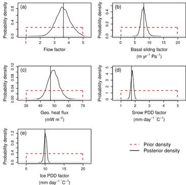
1 2 3 4 5
0.0 0.4 0.8 Flow factor Probability density (a)
0 5 10 15 20
0.0
0.2
0.4
Basal slidng factor
Probability density
(b)
(m yr−1 Pa−1)
30 40 50 60 70
0.00
0.04
0.08
0.12
Geo. heat flux
Probability density
(c)
(mW m−2)
1 2 3 4 5
0 1 2 3 4 5
Snow PDD factor
Probability density
(d)
(mm day−1°C−1)
5 10 15 20
0.0
0.4
0.8
1.2
Ice PDD factor
Probability density
(e)
(mm day−1°C−1)
Prior density Posterior density
Figure 3. Prior (dashed red curves) and posterior (solid black curves) probability density functions of each input parameter, as-suming that all the other parameters are held fixed at their assumed-true values. The vertical lines indicate the assumed-assumed-true values of the individual parameters. See Fig. S2 in the Supplement for the effect of excluding the discrepancy term (δin Eq. 1) on the results.
averaged ice thickness vectors are minor. Thus, our methods pass check no. 1, above.
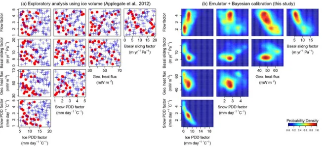
Similarly, the conditional posterior density functions (Fig. 3) have maxima near the assumed-true parameter val-ues. Parameter combinations yielding zonally averaged ice thickness curves that lie close to the assumed-true model re-alization (e.g., the red curve in Fig. 1) are more likely (more probable based on the posterior distribution) than those with curves that lie farther from the assumed-true values (blue and green curves in Fig. 1). We do not expect that the modes of the marginal posterior density functions (Fig. 4b) will fall ex-actly at the assumed-true parameter values because summing over one or more dimensions often moves the marginal mode away from the maximum of the multidimensional probability density function. In any case, the maximum posterior prob-ability is close to the assumed-true parameter combination. Thus, our methods pass check no. 2, above. Some of the two-dimensional marginal probability density functions (Fig. 4b) show multiple modes and bands of high probability extend-ing across the two-dimensional fields; we discuss the signifi-cance of these features below.
clustering around the assumed-true parameter values, except for the ice positive degree-day factor.
Our method also successfully recovers the ice volume loss produced by the assumed-true model realization (Fig. 5; see also Fig. S5 in the Supplement), reflected by the close corre-spondence between the mode of the probability density func-tion produced by our methods and the vertical black line. Thus, our methods pass check no. 3, listed above. As pre-viously noted, these projections are based on synthetic data; they are not “real” projections of Greenland Ice Sheet mass loss. For comparison, we also applied the windowing ap-proach used by Applegate et al. (2012) to the model runs and the synthetic observation. The 95 % probable interval pro-duced by our methods is much smaller than that estimated by computing the 2.5th and the 97.5th percentiles of the syn-thetic volume change values selected by the 10 % volume filter used in Applegate et al. (2012). This reflects the utility of spatial information and our probabilistic calibration ap-proach in reducing projection uncertainties compared to the windowing approach in Applegate et al. (2012).
The prior density for the ice volume loss was constructed by assuming that all 99 design points used to train our emula-tor are equally likely. Interestingly, a uniform prior for the in-put parameters results in a skewed and multimodal prior dis-tribution for the volume loss, indicating that the function that maps input parameters to projected ice volume changes is highly non-linear and not smooth. These characteristics also cause a small offset between the assumed-true projection and the mode of the posterior density. The marginal plots for the volume loss projection surfaces are shown in Fig. S3 in the Supplement.
4 Discussion
As explained above, our goals for this work were to identify an objective function for matching ice sheet models to spa-tially distributed data (especially ice thicknesses), map inter-actions among model input parameters, and develop meth-ods for projecting future ice sheet mass loss, with well-characterized uncertainties. We demonstrated that our emu-lator reproduces a vector of zonally averaged ice thicknesses from a given model run when trained on other members from the same ensemble (Fig. 2). We further showed that the emu-lator can recover the appropriate parameter combinations for an assumed-true model realization in a perfect model exper-iment (Figs. 3, 4b). Finally, we produced illustrative projec-tions of Greenland Ice Sheet mass loss based on synthetic data (Fig. 5; see also Fig. S5 in the Supplement). As noted above, our projections are for illustration only and do not rep-resent “real” projections of future Greenland Ice Sheet mass loss.
The utility of our approach becomes clear in comparing the marginal posterior probability density functions (Fig. 4b) and projections (red probability density function and box plot
in Fig. 5) to results from simpler methods (Fig. 4a; blue box plot in Fig. 5; Applegate et al., 2012). In Fig. 4b, there are distinct modes in the marginal densities, indicating re-gions of parameter space that are more consistent with the assumed truth. These modes are absent in the simpler graphic (Fig. 4a). Similarly, the 95 % prediction interval of sea level rise contributions is narrower using our methods than if a simple windowing approach is applied (Fig. 5). Our results also show the importance of including the discrepancy term (δin Eq. 1) for recovering the appropriate parameter settings in our perfect model experiments (Fig. S2 in the Supple-ment). If we leave this discrepancy term out, the marginal posterior density functions for each parameter clearly miss the true values.
The parameter interactions identified in this experiment are generally consistent with intuition (see Sect. 1.2 for de-scriptions of anticipated parameter interactions). Figure 4 shows inclined bands of high marginal posterior probability in the ice positive day factor vs. snow positive degree-day factor, geothermal heat flux vs. ice flow factor, and basal sliding factor vs. flow factor panels. As expected, there are tradeoffs among each of these parameter pairs; for example, a low ice positive degree-day factor must be combined with a high snow positive degree-day factor to produce a reason-able match to the assumed truth. Somewhat surprisingly, the tradeoff between the geothermal heat flux and the ice flow factor is much stronger than that between the geothermal heat flux and the basal sliding factor. The geothermal heat flux af-fects both ice deformation (which is temperature-sensitive) and basal sliding (which operates only where there is liq-uid water at the ice–bed interface). We hypothesize that the geothermal heat flux has a stronger effect on ice flow than basal sliding because ice deformation happens over a much larger fraction of the ice sheet’s basal area than does sliding. Multiple modes appear in the two-dimensional marginal density plots (Fig. 4), implying that standard methods for tuning of ice sheet models may converge to “non-optimal” parameter combinations. Ice sheet models are commonly tuned by manually adjusting one parameter at a time until the simulated modern ice sheet resembles the real one (e.g., Greve et al., 2011). This procedure is an informal variant of so-called gradient descent methods, which search for optimal matches between models and data by moving down a contin-uous surface defined by the model’s input parameters, the objective function, and the data. If the surface has multiple “peaks” (i.e., regions of parameter space that are more plau-sible, given observations, than their surroundings), gradient descent methods can converge to a point which produces a better match to the data than any adjacent point, but is never-theless far from the “best” parameter combination.
Figure 4.Comparison between an exploratory data analysis, following Applegate et al. (2012), and the results of our probabilistic calibration. Scatterplots of parameter settings used to train the emulator, as projected onto two-dimensional marginal spaces(a). Red dots are parameter settings resulting in simulated modern ice volumes within 10 % of the synthetic truth (model run #67 of Applegate et al., 2012); blue crosses are parameter settings that yield ice volumes more than 10 % larger or smaller than the synthetic truth. Two-dimensional marginal posterior densities of all pairs of input parameters(b). Several of the marginal posterior density maps show inclined bands of higher probability, indicating interactions among parameters; other panels show multiple modes, representing potential “traps” for tuning of ice sheet models using simpler methods. See text for discussion.
et al., 2013; Edwards et al., 2014a) used a variety of ice sheet models to project future ice sheet contributions to sea level rise. The two projects used different groups of ice sheet models and different methods for spinning up the partici-pating models. The results of one of these projects shows strong divergence among the results from different models (Bindschadler et al., 2013), whereas the other project’s pro-jections agree more closely (Shannon et al., 2013; Edwards et al., 2014a). The multiple modes in our posterior two-dimensional density plots (Fig. 4) suggest that some of the di-vergence among models, for example in the SeaRISE project (Bindschadler et al., 2013), may be due to differences in model tuning: even if the models had similar structures and reproduced the modern ice sheet topography and ice thick-nesses equally well, we would still expect their future pro-jections to diverge because of differences in input parameter choice.
Our leave-one-out cross-validation shows that the results presented here are consistent across all 100 synthetic truths. The prediction interval for the ice volume changes in Fig. 5 achieves the nominal coverage when the synthetic truth yields a modern ice volume that is close to the observed mod-ern ice volume (Fig. S5 in the Supplement). The parameter interactions shown in Fig. 4 are also consistent across the majority of the synthetic truths (Fig. S6 in the Supplement).
4.1 Caution and future directions
In this paper, we specifically avoid giving “real” projec-tions of future Greenland Ice Sheet volume change, for
two reasons. First, we match only a two-dimensional pro-file of zonally averaged ice thicknesses from an assumed-true model run, rather than the two-dimensional grid of observed ice thicknesses (Bamber et al., 2001, 2013; see also McNeall et al., 2013). Second, the ensemble of ice sheet model runs (Applegate et al., 2012) that we use to calibrate our emulator has several important limitations, including the relative sim-plicity of the model used to generate the ensemble and the synthetic climate scenario used to drive the ensemble mem-bers into the future. Most importantly, this ensemble’s simu-lated modern ice sheets are generally too thick in the south-ern part of Greenland and too thin in the northsouth-ern part of the island (Applegate et al., 2012, their Fig. 7); other studies that allow the ice sheet surface to evolve freely have noted similar difficulties in reproducing the modern ice sheet (e.g., Stone et al., 2010; Greve et al., 2011; Nowicki et al., 2013, their Fig. 2; cf. Edwards et al., 2014a). The long-term goal of this work is to compare ice sheet model runs to actual data, thereby resulting in probabilistic projections of future ice sheet mass loss. To achieve this goal, we plan to expand our method to treat the full, two-dimensional ice thickness grid and take advantage of other spatially distributed data sets (e.g., surface velocities; Joughin et al., 2010) and to generate new ice sheet model ensembles that overcome the limitations explained above.
5 Conclusions
−0.15 −0.10 −0.05 0.00
0
10
20
30
40
50
60
Illustrative projections based on synthetic data
ice volume change [m sle]
probability density
( )
( )
assumed true projection current approach Applegate et al. (2012) no calibration
Figure 5.Illustrative (not “real”) ice volume change projections be-tween 2005 and 2100, based on three different methods: (i) the prior density of the input parameters (dashed green line); (ii) parameter settings that pass the 10 % ice volume filter used by Applegate et al. (2012) (solid blue line); and (iii) the posterior density computed by our calibration approach (solid red line). The vertical line shows the ice volume change projection for the assumed-true parameter setting. The horizontal lines and the parentheses on them represent the range and the 95 % prediction intervals, respectively; the crosses indicate the median projection from each method. The width of the 95 % projection interval from our methods is narrower than if sim-pler methods are applied (blue box plot; Applegate et al., 2012). Similar results are obtained if different model runs from the ensem-ble are left out (see Fig. S5 in the Supplement). See text for discus-sion. The notation m sle stands for meters of sea level equivalent.
thickness information. Specifically, we constructed a prob-ability model for assigning posterior probabilities to indi-vidual ice sheet model runs, and we used a Gaussian pro-cess emulator to interpolate between existing ice sheet model simulations. We reduced the dimensionality of the emula-tion problem by reducing profiles of mean ice thicknesses to their principal components. Finally, we showed how the pos-terior probabilities from the model calibration exercise can be used to make projections of future sea level rise from the ice sheets. In a perfect model experiment where the “true” parameter settings and future contributions of the ice sheet to sea level rise are known, our methods successfully recovered these values. The posterior probability density function that resulted from this experiment shows tradeoffs among param-eters and multiple modes. The tradeoffs are consistent with physical expectations, whereas the multiple modes may in-dicate that commonly applied methods for tuning ice sheet models can lead to calibration errors.
The Supplement related to this article is available online at doi:10.5194/gmd-7-1933-2014-supplement.
Author Contributions
W. Chang designed the emulator, carried out the analyses, and wrote the first draft of the Supplement. P. J. Applegate wrote the first draft of the body text and supplied the pre-viously published ice sheet model runs (available online at http://bolin.su.se/data/Applegate-2011). W. Chang, P. J. Ap-plegate, M. Haran, and K. Keller jointly designed the re-search and edited the paper text.
Acknowledgements. We thank R. Greve for distribut-ing his ice sheet model SICOPOLIS freely on the Web (http://sicopolis.greveweb.net/) and N. Kirchner for help in setting up and using the model. R. Alley and D. Pollard provided helpful comments on a draft of the manuscript. This work was partially supported by the US Department of Energy, Office of Science, Biological and Environmental Research Program, Integrated Assessment Program, grant no. DE-SC0005171; by the US National Science Foundation through the Network for Sustainable Climate Risk Management (SCRiM) under NSF cooperative agreement GEO-1240507; and by the Penn State Center for Climate Risk Management. Any opinions, findings, and conclusions expressed in this work are those of the authors, and do not necessarily reflect the views of the National Science Foundation or the Department of Energy.
Edited by: I. Rutt
References
Alexander, L. V., Allen, S. K., Bindoff, N. L., Bron, F. M., Church, J. A., Cubasch, U., Emori, S., Forster, P., Friedlingstein, P., Gillett, N., Gregory, J. M., Hartmann, D. L., Jansen, E., Kirt-man, B., Knutti, R., Kanikicharla, K. K., Lemke, P., Marotzke, J., Masson-Delmotte, V., Meehl, G. A., Mokhov, I. I., Piao, S., Plattner, G. K., Dahe, Q., Ramaswamy, V., Randall, D., Rhein, M., Rojas, M., Sabine, C., Shindell, D., Stocker, T. F., Talley, L. D., Vaughan, D. G., and Xie, S. P.: Climate Change 2013: The Physical Science Basis: Contribution of Working Group I to the Fifth Assessment Report of the Intergovernmental Panel on Cli-mate Change, IPCC, Cambridge University Press, Cambridge, 2013.
Alley, R. B., Andrews, J. T., Brigham-Grette, J., Clarke, G. K. C., Cuffey, K. M., Fitzpatrick, J. J., Funder, S., Marshall, S. J., Miller, G. H., Mitrovica, J. X., Muhs, D. R., Otto-Bliesner, B. L., Polyak, L., and White, J. W. C.: History of the Greenland Ice Sheet: paleoclimatic insights, Quaternary Sci. Rev., 29, 1728– 1756, 2010.
Applegate, P. J., Kirchner, N., Stone, E. J., Keller, K., and Greve, R.: An assessment of key model parametric uncertainties in projec-tions of Greenland Ice Sheet behavior, The Cryosphere, 6, 589– 606, doi:10.5194/tc-6-589-2012, 2012.
Measure-ment, data reduction, and errors, J. Geophys. Res., 106, 33773– 33780, 2001.
Bamber, J. L., Griggs, J. A., Hurkmans, R. T. W. L., Dowdeswell, J. A., Gogineni, S. P., Howat, I., Mouginot, J., Paden, J., Palmer, S., Rignot, E., and Steinhage, D.: A new bed elevation dataset for Greenland, The Cryosphere, 7, 499–510, doi:10.5194/tc-7-499-2013, 2013.
Bindschadler, R. A., Nowicki, S., Abe-Ouchi, A., Aschwanden, A., Choi, H., Fastook, J.,Granzow, G., Greve, R., Gutowski, G., Herzfeld, U., Jackson, C., Johnson, J., Khroulev, C., Levermann, A., Lipscomb, W. H., Martin, M. A., Morlighem, M., Parizek, B. R., Pollard, D., Price, S. F., Ren, D., Saito, F., Sato, T., Seddik, H., Seroussi, H., Takahashi, K., Walker, R., and Wang, W. L.: Ice-sheet model sensitivities to environmental forcing and their use in projecting future sea level (the SeaRise project), J. Glaciol., 59, 195–224, 2013.
Born, A. and Nisancioglu, K. H.: Melting of Northern Greenland during the last interglaciation, The Cryosphere, 6, 1239–1250, doi:10.5194/tc-6-1239-2012, 2012.
Braithwaite, R. J.: Positive degree-day factors for ablation on the Greenland ice sheet studied by energy-balance modelling, J. Glaciol., 41, 153–160, 1995.
Brooks, S., Gelman, A., Jones, G., and Meng, X.-L. (Eds.): Hand-book of Markov Chain Monte Carlo, Chapman and Hall/CRC, 619 pp., 2011.
Calov, R. and Greve, R.: A semi-analytical solution for the posi-tive degree-day model with stochastic temperature variations, J. Glaciol., 51, 173–175, 2005.
Chang, W., Haran, M., Olson, R., and Keller, K.: Fast dimension-reduced climate model calibration, Ann. Appl. Stat., 8, 649–673, 2014.
Church, J. A. and White, N. J.: A 20th century acceleration in global sea-level rise, Geophys. Res. Lett., 33, L01602, doi:10.1029/2005GL024826, 2006.
Dansgaard, W., Johnsen, S. J., Clausen, H. B., Dahl-Jensen, D., Gundestrup, N. S., Hammer, C. U., Hvidberg, C. S., Steffensen, J. P., Sveinbjörnsdottir, A. E., Jouzel, J., and Bond, G.: Evidence for general instability of past climate from a 250-kyr ice core record, Nature, 364, 218–220, 1993.
Edwards, T. L., Fettweis, X., Gagliardini, O., Gillet-Chaulet, F., Goelzer, H., Gregory, J. M., Hoffman, M., Huybrechts, P., Payne, A. J., Perego, M., Price, S., Quiquet, A., and Ritz, C.: Effect of uncertainty in surface mass balance-elevation feedback on pro-jections of the future sea level contribution of the Greenland ice sheet, The Cryosphere, 8, 195–208, doi:10.5194/tc-8-195-2014, 2014a.
Edwards, T. L., Fettweis, X., Gagliardini, O., Gillet-Chaulet, F., Goelzer, H., Gregory, J. M., Hoffman, M., Huybrechts, P., Payne, A. J., Perego, M., Price, S., Quiquet, A., and Ritz, C.: Probabilis-tic parameterisation of the surface mass balance-elevation feed-back in regional climate model simulations of the Greenland ice sheet, The Cryosphere, 8, 181–194, doi:10.5194/tc-8-181-2014, 2014b.
Fitzgerald, P. W., Bamber, J. L., Ridley, J. K., and Rougier, J. C.: Exploration of parametric uncertainty in a surface mass balance model applied to the Greenland ice sheet, J. Geophys. Res., 117, F01021, doi:10.1029/2011JF002067, 2012.
Fyke, J. G., Weaver, A. J., Pollard, D., Eby, M., Carter, L., and Mackintosh, A.: A new coupled ice sheet/climate model:
de-scription and sensitivity to model physics under Eemian, Last Glacial Maximum, late Holocene and modern climate condi-tions, Geosci. Model Dev., 4, 117–136, doi:10.5194/gmd-4-117-2011, 2011.
Gillet-Chaulet, F., Gagliardini, O., Seddik, H., Nodet, M., Du-rand, G., Ritz, C., Zwinger, T., Greve, R., and Vaughan, D. G.: Greenland ice sheet contribution to sea-level rise from a new-generation ice-sheet model, The Cryosphere, 6, 1561–1576, doi:10.5194/tc-6-1561-2012, 2012.
Gladstone, R. M., Lee, V., Rougier, J., Payne, A. J., Hellmer, H., Le Brocq, A., Shepherd, A., Edwards, T. L., Gregory, J., and Cornford, S. L.: Calibrated prediction of Pine Island Glacier retreat during the 21st and 22nd centuries with a cou-pled flowline model, Earth Planet. Sc. Lett., 333–334, 191–199, doi:10.1016/j.epsl.2012.04.022, 2012.
Goelzer, H., Huybrechts, P., Fürst, J. J., Nick, F. M., Andersen, M. L., Edwards, T. L., Fettweis, X., Payne, A. J., and Shannon, S.: Sensitivity of Greenland ice sheet projections to model formula-tions, J. Glaciol., 59, 1–17, doi:10.3189/2013JoG12J182, 2013. Greve, R.: Application of a polythermal three-dimensional ice sheet
model to the Greenland Ice Sheet: response to steady-state and transient climate scenarios, J. Climate, 10, 901–918, 1997. Greve, R. and Otsu, S.: The effect of the north-east ice stream on
the Greenland ice sheet in changing climates, The Cryosphere Discuss., 1, 41–76, doi:10.5194/tcd-1-41-2007, 2007.
Greve, R., Saito, F., and Abe-Ouchi, A.: Initial results of the SeaRISE numerical experiments with the models SICOPOLIS and IcIES for the Greenland Ice Sheet, Ann. Glaciol., 52, 23–30, 2011.
Hastings, W. K.: Monte Carlo sampling methods using Markov chains and their applications, Biometrika, 57, 97–109, 1970. Hebeler, F., Purves, R. S., and Jamieson, S. S. R.: The impact of
parametric uncertainty and topographic error in ice-sheet mod-elling, J. Glaciol., 54, 899–919, 2008.
Heimbach, P. and Bugnion, V.: Greenland ice-sheet volume sen-sitivity to basal, surface and initial conditions derived from an adjoint model, Ann. Glaciol., 50, 67–80, 2009.
Huybrechts, P.: Sea-level changes at the LGM from ice-dynamic reconstructions of the Greenland and Antarctic ice sheets during the glacial period, Quaternary Sci. Rev., 21, 203–231, 2002. Imbrie, J., Hays, J. D., Martinson, D. G., McIntyre, A., Mix, A. C.,
Morley, J. J., Pisias, N. G., Prell, W. L., and Shackleton, N. J.: The orbital theory of Pleistocene climate: support from a revised chronology of the marineδ18O record, in: Milankovitch and cli-mate: understanding the response to astronomical forcing, Part 1, edited by: Berger, A. J., Imbrie, J., Hays, J., Kukla, G., and Saltz-man, B., D. Reidel Publishing Co., Dordrecht, 269–305, 1984. Jevrejeva, S., Moore, J. C., Grinsted, A., and Woodworth, P. L.:
Re-cent global sea level acceleration started over 200 years ago?, Geophys. Res. Lett., 35, L08715, doi:10.1029/2008GL033611, 2008.
Joughin, I., Smith, B. E., Howat, I. M., Scambos, T., and Moon, T.: Greenland flow variability from ice-sheet-wide velocity map-ping, J. Glaciol., 56, 415–430, 2010.
Kennedy, M. C. and O’Hagan, A.: Bayesian calibration of computer models, J. Roy. Stat. Soc. B Met., 63, 425–464, 2001.
Kirchner, N., Hutter, K., Jakobsson, M., and Gyllencreutz, R.: Ca-pabilities and limitations of numerical ice sheet models: a discus-sion for Earth-scientists and modelers, Quaternary Sci. Rev., 30, 3691–3704, 2011.
Lemke, P., Ren, J., Alley, R. B., Allison, I., Carrasco, J., Flato, G., Fujii, Y., Kaser, G., Mote, P., Thomas, R. H., and Zhang, T.: Ob-servations: changes in snow, ice, and frozen ground, edited by: Solomon, S., Qin, D., Manning, M., Chen, Z., Marquis, M., Av-eryt, K. B., Tignor, M., and Miller, H. L., Cambridge University Press, Cambridge, 2007.
Lempert, R., Sriver, R. L., and Keller, K.: Characterizing uncertain sea level rise projections to support investment decisions, Cali-fornia Energy Commission Report CEC-500-2012-056, 2012. Lenton, T. M., Held, H., Kriegler, E., Hall, J. W., Lucht, W.,
Rahm-storf, S., and Schnellnhuber, H. J.: Tipping elements in the Earth’s climate system, P. Natl. Acad. Sci. USA, 105, 1786– 1793, 2008.
Little, C. M., Oppenheimer, M., Urban, N. M.: Upper bounds on twenty-first-century Antarctic ice loss assessed using a probabilistic framework, Nature Climate Change 3, 654–659, doi:10.1038/nclimate1845, 2013.
McKay, M. D., Beckman, R. J., and Conover, W. J.: A compari-son of three methods for selecting values of input variables in the analysis of output from a computer code, Technometrics, 21, 239–245, 1979.
McNeall, D. J., Challenor, P. G., Gattiker, J. R., and Stone, E. J.: The potential of an observational data set for calibration of a com-putationally expensive computer model, Geosci. Model Dev., 6, 1715–1728, doi:10.5194/gmd-6-1715-2013, 2013.
Meehl, G. A., Stocker, T. F., Collins, W. D., Friedlingstein, P., Gaye, A. T., Gregory, J. M., Kitoh, A., Knutti, R., Murphy, J. M., Noda, A., Raper, S. C. B., Watterson, I. G., Weaver, A. J., and Zhao, Z.-C.: Global climate projections, edited by: Solomon, S., Qin, D., Manning, M., Chen, Z., Marquis, M., Averyt, K. B., Tignor, M., and Miller, H. L., Cambridge University Press, Cambridge, 2007.
Nowicki, S., Bindschadler, R. A., Abe-Ouchi, A., Aschwanden, A., Bueler, E., Choi, H., Fastook, J., Granzow, G., Greve, R., Gutowski, G., Herzfeld, U., Jackson, C., Johnson, J., Khroulev, C., Larour, E., Levermann, A., Lipscomb, W. H., Martin, M. A., Morlighem, M., Parizek, B. R., Pollard, D., Price, S. F., Ren, D., Rignot, E., Saito, F., Sato, T., Seddik, H., Seroussi, H., Takahashi, K., Walker, R., and Wang, W. L.: Insights into spatial sensitivities of ice mass response to environmental change from the SeaRISE ice sheet modeling project II: Greenland, J. Geophys. Res.-Earth, 118, 1025–1044, doi:10.1002/jgrf.20076, 2013.
Pollard, D. and DeConto, R. M.: A simple inverse method for the distribution of basal sliding coefficients under ice sheets, applied to Antarctica, The Cryosphere, 6, 953–971, doi:10.5194/tc-6-953-2012, 2012.
Quiquet, A., Punge, H. J., Ritz, C., Fettweis, X., Gallée, H., Kageyama, M., Krinner, G., Salas y Mélia, D., and Sjolte, J.: Sensitivity of a Greenland ice sheet model to atmospheric forc-ing fields, The Cryosphere, 6, 999–1018, doi:10.5194/tc-6-999-2012, 2012.
Ritz, C., Fabre, A., and Letreguilly, A.: Sensitivity of a Green-land Ice Sheet model to ice flow and ablation parameters: con-sequences for the evolution through the last climatic cycle, Clim. Dynam., 13, 11–24, 1997.
Robinson, A., Calov, R., and Ganopolski, A.: An efficient regional energy-moisture balance model for simulation of the Greenland Ice Sheet response to climate change, The Cryosphere, 4, 129– 144, doi:10.5194/tc-4-129-2010, 2010.
Rutt, I. C., Hagdorn, M., Hulton, N. R. J., and Payne, A. J.: The Glimmer community ice-sheet model, J. Geophys. Res.-Earth, 114, F02004, doi:10.1029/2008JF001015, 2009.
Sacks, J., Welch, W. J., Mitchell, T. J., and Wynn, H. P.: Design and analysis of computer experiments (with discussion), J. Stat. Sci., 4, 409–423, 1989.
Seddik, H., Greve, R., Zwinger, T., Gillet-Chaulet, F., and Gagliar-dini, O.: Simulations of the Greenland ice sheet 100 years into the future with the full Stokes model Elmer/Ice, J. Glaciol., 58, 427–440, 2012.
Shannon, S. R., Payne, A. J., Bartholomew, I. D., van den Broeke, M. R., Edwards, T. L., Fettweis, X., Gagliardini, O., Gillet-Chaulet, F., Goelzer, H., Hoffman, M. J., Huybrechts, P., Mair, D. W. F., Nienow, P., Perego, M., Price, S. F., Smeets, C. J. P. P., Sole, A. J., van de Wal, R. S. W., and Zwinger, T.: En-hanced basal lubrication and the contribution of the Greenland ice sheet to future sea-level rise, P. Natl. Acad. Sci., 110, 1–4, doi:10.1073/pnas.1212647110, 2013.
Stone, E. J., Lunt, D. J., Rutt, I. C., and Hanna, E.: Investigating the sensitivity of numerical model simulations of the modern state of the Greenland ice-sheet and its future response to climate change, The Cryosphere, 4, 397–417, doi:10.5194/tc-4-397-2010, 2010. Urban, N. M. and Fricker, T. E.: A comparison of Latin hypercube
and grid ensemble designs for the multivariate emulation of an Earth system model, Comput. Geosci., 36, 746–755, 2010. van der Berg, W. J., van den Broeke, M., Ettema, J., van
Meij-gaard, E., and Kaspar, F.: Significant contribution of insolation to Eemian melting of the Greenland ice sheet, Nat. Geosci., 4, 679–683, 2011.