The Cryosphere, 7, 183–199, 2013 www.the-cryosphere.net/7/183/2013/ doi:10.5194/tc-7-183-2013
© Author(s) 2013. CC Attribution 3.0 License.
Geoscientiic
Geoscientiic
Geoscientiic
Geoscientiic
The Cryosphere
Open Access
Effect of higher-order stress gradients on the centennial mass
evolution of the Greenland ice sheet
J. J. F ¨urst, H. Goelzer, and P. Huybrechts
Vrije Universiteit Brussel, Earth System Sciences and Departement Geografie, Pleinlaan 2, Brussel, Belgium Correspondence to:J. J. F¨urst ([email protected]), H. Goelzer ([email protected]),
and P. Huybrechts ([email protected])
Received: 26 June 2012 – Published in The Cryosphere Discuss.: 27 July 2012
Revised: 19 November 2012 – Accepted: 27 December 2012 – Published: 1 February 2013
Abstract.We use a three-dimensional thermo-mechanically coupled model of the Greenland ice sheet to assess the ef-fects of marginal perturbations on volume changes on cen-tennial timescales. The model is designed to allow for five ice dynamic formulations using different approximations to the force balance. The standard model is based on the shallow ice approximation for both ice deformation and basal slid-ing. A second model version relies on a higher-order Blat-ter/Pattyn type of core that resolves effects from gradients in longitudinal stresses and transverse horizontal shearing, i.e. membrane-like stresses. Together with three intermedi-ate model versions, these five versions allow for gradually more dynamic feedbacks from membrane stresses. Idealised experiments are conducted on various resolutions to compare the time-dependent response to imposed accelerations at the marine ice front. If such marginal accelerations are to have an appreciable effect on total mass loss on a century timescale, a fast mechanism to transmit such perturbations inland is re-quired. While the forcing is independent of the model ver-sion, inclusion of direct horizontal coupling allows the initial speed-up to reach several tens of kilometres inland. Within one century, effects from gradients in membrane stress al-ter the inland signal propagation and transmit additional dy-namic thinning to the ice sheet interior. But the centennial overall volume loss differs only by some percents from the standard model, as the dominant response is a diffusive in-land propagation of geometric changes. For the experiments considered, this volume response is even attenuated by direct horizontal coupling. The reason is a faster adjustment of the sliding regime by instant stress transmission in models that account for the effect of membrane stresses. Ultimately, hor-izontal coupling decreases the reaction time to perturbations
at the ice sheet margin. These findings suggest that for mod-elling the mass evolution of a large-scale ice sheet, effects from diffusive geometric adjustments dominate effects from successively more complete dynamic approaches.
1 Introduction
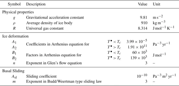
Table 1.Parameter overview.
Symbol Description Value Unit
Physical properties
g Gravitational acceleration constant 9.81 m s−2 ρ Average density of ice body 910 kg m−3 R Universal gas constant 8.314 J mol−1K−1 Ice deformation
A1 Coefficients in Arrhenius equation for T•< Tc 3.99×10⁻⁵
Pa−3yr−1 A2 T•> Tc 1.91×10¹¹
B1 Factors in Arrhenius equation for T•< Tc 60×103
J mol−1
B2 T•> Tc 139×103
n Exponent in Glen’s flow equation 3 – Basal Sliding
Asl Sliding coefficient 10−10 Pa−3m2yr−1
m Exponent in Budd/Weertman type sliding law 3 –
Howat and Eddy, 2011) while for other areas, a more er-ratic behaviour is found (Howat et al., 2010; Joughin et al., 2010; McFadden et al., 2011; Moon et al., 2012). This in-homogeneity impedes the identification of the most relevant trigger mechanisms. Hypotheses range from enhanced basal lubrication by increased summer melt (Zwally et al., 2002; Joughin et al., 2008; Bartholomew et al., 2010; Sundal et al., 2011; Schoof, 2010), to cryo-hydrologic warming by melt drainage (Phillips et al., 2010), ocean-induced grounding line retreat (Schoof, 2007; Briner et al., 2009) or enhanced calv-ing activity (Benn et al., 2007; Nick et al., 2010). Loss of buttressing at the glacier front is believed to be induced ei-ther by local surface melt (Scambos et al., 2000), by hydro-fracturing and subsequent front destabilisation, or by intru-sion of warm, saline ocean water into the local fjord systems, causing submarine melting (Holland et al., 2008; Amund-son et al., 2010; Straneo et al., 2010, 2011; Motyka et al., 2011; Christofferson et al., 2011). Except for cyclic surge be-haviour, observations indicate that accelerations mostly orig-inate in the marine-termorig-inated ablation area. This area con-stitutes a small fraction of the entire GrIS and instant ef-fects from speed-up remain confined to the periphery. Such marginal perturbations are directly and indirectly transmit-ted inland by ice dynamics and the efficiency of this signal transmission controls the impact on the interior (Nick et al., 2009).
One indirect mechanism for signal transmission is diffu-sive surface elevation adjustment. Marginal perturbations al-ter the local ice thickness and surface slope, which in turn affects the flow in the immediate vicinity. The surrounding geometry consequently adjusts and thereby the signal is grad-ually transmitted inland. The effects of such diffusive geom-etry adjustments are well understood and have been studied in models for large-scale ice sheets both on long and short time-scales (Huybrechts and de Wolde, 1999; Ritz et al., 2001). However, there are also direct mechanisms that can
instantaneously transmit marginal perturbations inland. One potential candidate for direct signal transmission is inherent in the force balance within a solid body of ice. Gradients in membrane-like stresses (cf. Hindmarsh, 2006) allow for such direct horizontal coupling. These stresses are often referred to as “longitudinal stresses” owing to an extensive study on flow bands.
From a theoretical point, longitudinal coupling in an ice sheet is efficient within a domain of four to ten times the ice thickness (Kamb and Echelmeyer, 1986). For the Green-land ice sheet we therefore expect values of 5 to 40 km. For a flow band setup on Jakobshavn Isbræ, Price et al. (2008) succeeded to explain instant accelerations observed at Swiss Camp by longitudinal transmission of near margin perturba-tions. With a linear flow and sliding law, they solve the full force balance equation and estimate that horizontal coupling has a 10–15 km area of direct influence. For a similar 2-D application on Helheim, Nick et al. (2009) highlight the tran-sient propagation of perturbations initiated at the glacier ter-minus. The immediate response confirms a 10 km coupling radius to the applied marginal forcing. The effective longi-tudinal coupling length increases when accounting for the nonlinear character of ice creep and basal sliding (Kamb and Echelmeyer, 1986; Price et al., 2008). For a typical fast flow-ing Antarctic ice stream, it can reach up to 40 km (Williams et al., 2012). Flow band geometries are however limited to the effect of longitudinal stress gradients and omit effects from transverse shearing, which occur widely in many stream-like outlet glaciers embedded in the GrIS. Moreover, the purpose of such flow line setups is often to reproduce observed flow evolution rather than the study of the influence of direct hor-izontal coupling on the geometry evolution.
J. J. F ¨urst et al.: Effects of higher-order stress gradients 185
Table 2.Overview of model versions with different approaches to describe ice deformation and basal resistance. Note that the ME HO combination is omitted in this work. Details to each approach are described in Sect. 2.3 and in Appendix B.
Ice Deformation
Shallow Ice Higher-order Approximation approach
Basal resistance
Driving
DR SIA DR HO Stress
Membrane
ME SIA (ME HO) Stresses
Simplified
SR SIA SR HO Resistance
the model is described in Sect. 2 together with a justifica-tion for its applicability to direct stress transmission. Sec-tion 3 sets the experimental frame for the centennial per-turbation scenarios on Greenland, while results are subse-quently discussed in Sect. 4. Introduction of an instant re-action timescale provides a tool to summarise results from all experiments for different resolutions and model versions in Sect. 5. Before the final conclusion, a discussion of the entire model setup assesses the reliability of the results.
2 Model description and terminology
2.1 Stress terminology
The fundamental force balance is presented in Appendix A and serves as a basis for the used stress terminology. Based on scaling arguments, vertical plane shearing (σxz,σyz) ex-erts major control on the dynamics of large-scale grounded ice bodies, as exemplified in the shallow ice approximation (SIA; Hutter, 1983). Following the terminology in Hind-marsh (2006), normal stresses acting in the horizontal di-rection (σxx,σyy) and horizontal shearing on vertical planes (σxy,σyx) are referred to as membrane-like or simply mem-brane stresses. Here we refer toσxx,σyy as the longitudinal stresses acting in the horizontal direction parallel to the nor-mal vector of the respectively addressed surface. The other two membrane stresses we refer to as transverse horizon-tal shear stresses (σxy,σyx), or simply transverse horizontal shearing. Their influence on ice dynamics is referred to as di-rect horizontal coupling or didi-rect stress/signal transmission. Note that this terminology is linked to the imposed coordi-nate system and is best applicable to large-scale geometries. For generalisation to more complex geometries, a consistent and precise terminology will depend on local geometry.
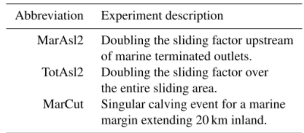
Table 3.Overview of the three perturbation experiments.
Abbreviation Experiment description
MarAsl2 Doubling the sliding factor upstream of marine terminated outlets. TotAsl2 Doubling the sliding factor over
the entire sliding area.
MarCut Singular calving event for a marine margin extending 20 km inland.
2.2 General model characteristics
The three-dimensional thermo-mechanically coupled ice sheet model comprises three main components that respec-tively describe the ice rheology, the Earth crust’s isostatic re-bound and the mass balance at the upper and lower ice sheet boundaries (Huybrechts and de Wolde, 1999; Huybrechts, 2002; to which the interested reader is referred for a de-tailed description of all model components). The optional higher-order (HO) ice-dynamic core is described in F¨urst et al. (2011). The surface mass balance model is based on the widely used positive degree-day/retention method. As input serves a generic temperature field, which depends on latitude and surface elevation, together with a temperature scaled pre-cipitation field (Huybrechts, 2002). Ice dynamics, isostatic adjustment and mass balance are implemented on a com-putational grid with 5 km horizontal resolution and 30 non-equidistant layers. The vertical grid spacing is refined to-wards the bottom where vertical plane shearing is concen-trated. Geometric input has been modified from the origi-nal Bamber et al. (2001) data as described in Huybrechts et al. (2011).
2.3 Model versions for ice dynamics
For ice deformation our model optionally applies the clas-sical SIA approach or an LMLa higher-order (HO) core (F¨urst et al., 2011). The latter version captures dynamic feedbacks arising from gradients in membrane stresses (cf. Sect. 2.1). These two options are combined with either of three possible descriptions of basal resistance. A first ap-proach assumes that basal resistance locally supports the driving stress (DR). A second approach uses the shallow shelf approximation as a sliding law (ME) (cf. Ritz et al., 2001; Bueler and Brown, 2009; Schoof and Hindmarsh, 2010). In this case, resistance at the base is dominated by membrane stresses while any effect from vertical shear-ing on slidshear-ing is neglected. Reconcilshear-ing these two extreme approaches, a simplified resistance (SR) equation includes effects from both vertical plane shearing and membrane stresses at the base. The simplification used in this third ap-proach is inherited from the HO ice deformation and stems from a scale analysis of gradients in the velocity field (cf. Appendix B).
Table 2 summarizes the five model versions that arise from combining these approximations used for ice creep and basal resistance. Note that the SR SIA model version actually needs a full determination of the 3-D higher-order solution in order to extract the velocity field at the base. In addition, the ME HO model version is not considered here because mem-brane stress activity for the basal and deformational part of ice dynamics is more self-consistent in SR HO.
3 Experimental design
The experimental frame for this study is set by three schematic perturbation scenarios and focuses on the centen-nial response of the GrIS. These experiments serve mainly as an intercomparison study for the five model versions with different dynamic complexity but they also give indications on the dynamic ice loss within one century. Optional grid spacing of 20, 10 or 5 km allows us to investigate the impact of resolution on capturing direct signal transmission.
3.1 Initialisation
An interglacial equilibrium state serves as the standard initial condition. The climatic forcing is obtained from a generic temperature field that depends on latitude and surface eleva-tion (details in Huybrechts, 2002). The initialisaeleva-tion on 5 km takes 25 kyr and is preceded by a 200 and a 100 kyr equilib-rium run on respectively 20 and 10 km. For this spin-up the DR SIA model setup is chosen and we denote this standard interglacial with “IS”. For assessing the robustness of the results under different initial conditions, we experimented with two other spin-up methods. The first one uses the SR HO model version to produce the interglacial equilibrium. It starts from the respective IS geometry and is evolved for ei-ther 50, 20 and 5 kyr to an initial state “IH”. For the third
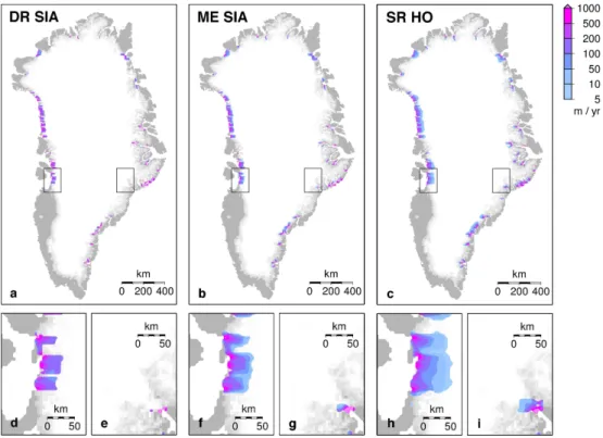
Fig. 1.Surface velocity magnitude for the IS standard interglacial equilibrium with continental outline in grey. The underlying geome-try is obtained with the DR SIA model.(a)and(c)show the velocity magnitude for DR SIA while their higher-order equivalent from SR HO is presented in(b)and(d)for the same geometry. The lower two panels(c)and(d)show a close-up around Kangerlussauq.
initialisation method, the model is spun up over the last two glacial cycles in the same way as described in Huybrechts et al. (2011). The resolution was successively increased from 20 km to 10 km at 20 kyr BP and to 5 km at 3 kyr BP.
3.2 Perturbation experiments
We conduct three experiments that address various aspects of Greenland’s ice dynamic response (cf. Table 3). Their focus is on the century timescale while they are designed in a way that each model version is applicable. The central experiment prescribes a step function in the basal sliding coefficientAsl
but spatially confines this amplification to the marine ter-minated boundary (experiment MarAsl2). Our choice for an
Aslamplification factor of 2 in grid boxes within 40 km
J. J. F ¨urst et al.: Effects of higher-order stress gradients 187
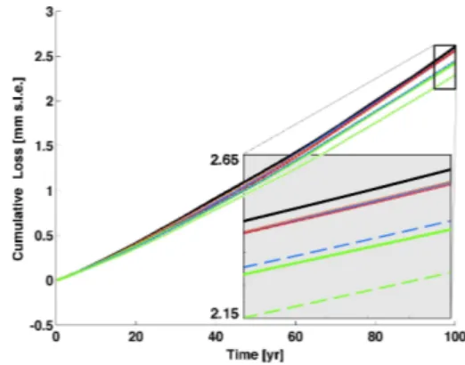
Fig. 2.Ice mass loss of different model versions on 5 km resolution for the three forcing scenarios:(a)MarAsl2,(c)TotAsl2,(d)MarCut started from IS while in panel(b)MarAsl2 is initiated from PS. Mass loss is determined by subtracting the background signal from a control experiment. The mass loss differs by no more than 20 % amongst the model versions and results are robust under different initial conditions
(a)and(b). Each close-up zooms in on the last 5 yr of the experiments. The dashed blue (ME SIA) and green (SR HO) line represent the respective model version using a full nonlinear sliding law (cf. Appendix B).
a marine boundary are instantaneously emptied. In order to ensure comparability between all resolutions ice removal is enforced up to 20 km inland.
To enable a clean comparison between the five model ver-sions, ice velocities in the first grounded point are based on the DR SIA model version. This provides unified pertur-bations for all experiments. Otherwise we would introduce numerical differences in the implementation of the lateral boundary conditions originating from the non-local influence on the velocity solution in model versions with horizontal coupling, which requires zero velocity outside the ice sheet. Although this approach inhibits membrane stress activity in the first grounded ice point, none of the used resolutions ac-tually resolve the complex stress situation in these zones. Additional tests (not shown) brought to light that applying the DR SIA lateral boundary condition at the first grounded point either all around Greenland or restricted to the marine margin has no significant influence on the presented results. Using SR HO at the lateral boundary, the qualitative differ-ences in volume evolution and in thickness response remain the same between models that use DR SIA and SR HO
up-stream. However, the centennial mass loss increases by 17 % with this second boundary condition but independently of model version. Unperturbed control runs are conducted to assess the effects of model adjustment and background evo-lution.
4 Results
underlines the gain from grid refinement. Note that the mod-elled stream features arise naturally from resolved details in bedrock topography and subglacial heating. They are not the result from optimising the basal sliding coefficient to match the observed velocity field as in Price et al. (2011).
In our setup, the IS surface velocity field is in equilib-rium with the DR SIA equations and the continuity equation. The velocity field computed with the SR HO variant for the same geometry largely resembles the DR SIA solution. Ef-fects from higher-order dynamics only become apparent in minor details of the ice flow (cf. Fig. 1). The DR SIA ve-locity magnitude exhibits sharper jagged features that are ef-fectively smoothed by direct horizontal coupling in the full higher-order version. Moreover the ice divide velocities tend to be higher in the SR HO version as a result of longitudi-nal stress transmission. Furthermore, effects from transverse horizontal shear are readily visible across narrow ice streams, where fast stream velocities couple with the stagnant ice in the surroundings (see e.g. Kangerlussauq, Fig. 1c, d).
In the following the transient effect of direct horizontal coupling is studied on various resolutions. First the GrIS vol-ume evolution is determined for all perturbation experiments (cf. Table 3). The GrIS mass loss for MarAsl2 is then decom-posed in a purely dynamic signal and a component arising from the feedback with surface mass balance. The dominant dynamic feedback is further investigated by comparing all model versions. Finally, results covering all model versions, grid resolutions and marginal perturbation experiments are analysed by introducing a reaction timescale to characterise their individual response behaviour.
4.1 Dynamic mass loss
For all experiments, the total volume loss of the GrIS after one century falls into a range of 1 and 12 cm eustatic sea-level equivalent (s.l.e.), cf. Fig. 2. This centimetre volume response is in line with estimates for present-day rates of in-creased ice export of about 0.2–0.4 mm s.l.e. yr−1(van den Broeke et al., 2009) and projections for future dynamic re-sponse (Price et al., 2011). The results have to be interpreted relative to Greenland’s total mass balance. The modelled net accumulation for the IS equilibrium geometry is equivalent to 1.5 mm s.l.e. yr−1. It is balanced by surface runoff and ice discharge at rates of 0.84 (55 %) and 0.66 mm s.l.e. yr−1 (45 %), respectively. Doubling of the sliding coefficient in DR SIA initially almost doubles the ice discharge and would therefore extrapolate to a centennial mass loss of about 66 mm s.l.e. in case such rates could be sustained. However, all experiments show that initial mass loss rates are not sus-tained. Even for a doubling of sliding over the entire sliding area (TotAsl2), upstream supply of ice is not sufficient to sus-tain the discharge rates. They gradually decrease and add up to a mass loss of 40 mm s.l.e. after one century (Fig. 2c). For MarAsl2 (Fig. 2a), initial mass loss rates abate even faster due to a lack of upstream inflow, adding up to 16 mm after
Fig. 3.Additional mass loss from changes in surface mass balance for the MarAsl2 experiment initiated from IS with respect to a con-trol run. This mass loss component increases almost linearly and higher-order dynamics reduce the magnitude.
one century. Similarly, the initial release of some 40 mm s.l.e. ice volume in the MarCut experiment is followed by a quick decrease in mass loss rates (Fig. 2d). Rerunning the MarAsl2 experiment from the IH interglacial or from the present PS state (cf. Fig. 2b) shows a qualitatively similar mass evolu-tion. On 20 km, the MarAsl2 experiment was repeated with amplification factors of five and ten (results not shown). The results indicate that the centennial mass loss scales almost linearly for such forcing magnitudes.
A comparison of the different model versions shows that the triggered mass losses are similar (Fig. 2). Differences lie within 20 % of the total signal, so that additional effects from the ice-dynamic complexity of each model version are generally small. For all experiments, an increase in dynamic complexity actually reduces the centennial mass loss. This negative feedback is especially strong when activating a full nonlinear sliding law (dashed lines in Fig. 2a) reaching 20 % of the total signal. This highlights the importance of sliding in attenuating the mass loss signal. This mass loss reduction is reproduced on all resolutions (cf. Sect. 4.4) and is robust under the various initial states.
J. J. F ¨urst et al.: Effects of higher-order stress gradients 189
Fig. 4.Initial response in surface velocities to the MarAsl2 perturbation for the three main model versions. Initiated from the 5 km IS, the geometry is still identical although theAslforcing already operates. Shown are accelerations with respect to a control experiment run for each
model version. In the DR SIA setup(a), the marginal accelerations are inherently confined to the forcing area. The close-ups of Jakobshavn Isbræ(d)and Kangerlussauq(e)allow the clear identification of the grid cells that experienceAslamplification. In the ME SIA(b, f, g)and
SR HO setup(c, h, i), direct horizontal coupling is included and effects from both longitudinal stresses and transverse horizontal shearing are distinguishable.
4.2 Inland propagation of marginal perturbations
For MarAsl2, the modelled reduction of ice discharge at the marine margin depends on the details of the upstream prop-agation of these accelerations. To investigate spatial differ-ences in successive geometric adjustment, we first analyse the initial velocity response. We conclude this section with a decomposition of the velocity response into its basal and deformational component.
The basal sliding coefficientAslis doubled within an area
extending 40 km inland from the marine ice front. The ini-tial response of the velocity field under identical geometries is shown in Fig. 4 for the three main and more commonly used model versions. In the DR SIA setup (Fig. 4a, d, e), accelerations are obviously limited to the actually perturbed grid points and allow a delineation of theAslamplification
zone. Note that the perturbation is additionally confined to the actual extent of the sliding area, which becomes visible for the close-ups on Jakobshavn Isbræ (Fig. 4d) and Kanger-lussauq (Fig. 4e). Including horizontal coupling, ME SIA (Fig. 4b, f, g) and SR HO (Fig. 4c, h, i) reveal how the initial acceleration instantaneously radiates some distance inland. Transverse horizontal shearing affects a vicinity of about 5–10 km for both model versions, whereas the
cou-pling length for longitudinal stress gradients seems larger. ME SIA exhibits values of about 20 km while SR HO ex-pands the coupling to more than 40 km (cf. Fig. 4f, g, h, i). For ice thicknesses of about one kilometre, these values are in broad agreement with the theoretical coupling length (Kamb and Echelmeyer, 1986). A greater coupling length is possible for high sliding or elongated, deep bed troughs as is the case for Kangerlussauq (Fig. 4e, g, i). For Jakobshavn Isbræ, Price et al. (2008) exemplarily demonstrate the positive influence of basal sliding on the longitudinal coupling length.
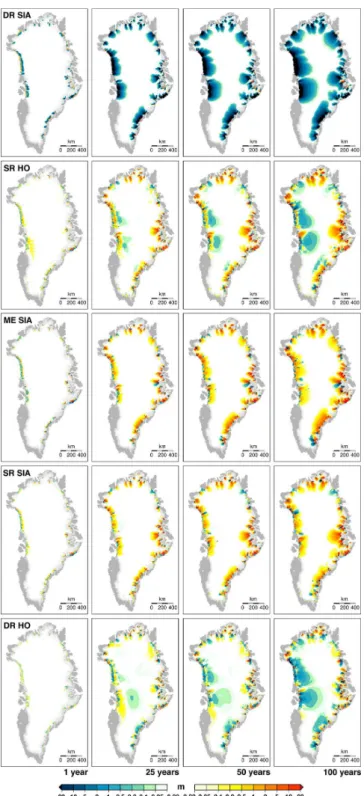
Fig. 5.Ice thickness evolution for the 5 km MarAsl2 experiment for all five model versions started from the IS state. The upper panels show the DR SIA ice thickness differences with respect to its control run after respectively 1, 25, 50 and 100 yr. Ice thickness changes in the other model versions are shown with respect to the dominant DR SIA differences.
Since diffusive thinning dominates the transient response in all model versions, their thickness evolutions are given with respect to the DR SIA reference. Initially, direct hori-zontal coupling hardly affects the geometric adjustment be-yond the area of diffusive thinning. But close to the marine margin horizontal coupling causes more pronounced thin-ning. In a later stage, its integrated effect shows up as an extra thinning signal in the interior, most pronounced for model versions that resolve vertical variations in membrane stresses (DR HO and SR HO). Yet in all models, a general thickening pattern emerges in the upper regions of the ab-lation zone, in between the zones of relative thinning. This spatial pattern appears to be a fingerprint of accounting for horizontal gradients in membrane stresses, especially when resolving them vertically (SR HO and DR HO). Though not decisively altering the mass loss response on centennial timescales, the additional thinning reduces the ice export and thus provides an explanation for the decreased total mass loss (cf. Fig. 2). The relative thickening of the upper ablation ar-eas arises from downstream damming by the thinned margin. But also upstream accelerations (see Fig. 6) add to this ice bulge, in particular for SR HO and DR HO. Since this rela-tive thickening is situated in the upper ablation region, a pos-itive feedback between surface elevation and mass balance amplifies this phenomenon (cf. also Huybrechts et al., 2002). After 50 yr of geometry evolution, our model versions branch out significantly and velocity fields also hold information on differences in integrated ice thickness changes (cf. Fig. 6). Prominent are the relative deceleration in the region of dy-namic thickening and the marginal speed-up. ME SIA re-stricts the effect from membrane stress gradients to the basal layer and velocity differences are dictated by the basal com-ponent. Consequently the deformational component hardly exceeds the area of basal velocity changes (Fig. 6a, c) and additional thinning further upstream remains negligible. In-terior thinning however is experienced in the SR HO model, where direct horizontal coupling throughout the entire verti-cal ice column transmits the acceleration beyond the sliding area extent (see Fig. 6b, d).
Altogether, the spatial propagation of marginal perturba-tions confirms that dynamic complexity indeed alters the ge-ometry evolution, but this is far outweighed by the dominant background thickness diffusion. Significant effects on geo-metric adjustment from direct horizontal stress transmission cannot be confirmed even in the case of full nonlinear sliding.
4.3 Decomposition of mass loss attenuation
J. J. F ¨urst et al.: Effects of higher-order stress gradients 191
Fig. 6.Differences in ice velocity changes for the 5 km MarAsl2 experiment after 50 yr for ME SIA(a, c)and SR HO(b, d). Surface (upper panels) and basal velocity changes (lower panels) are shown with respect to the changes in the DR SIA velocity evolution.
thicknessH and the velocity magnitudeV near the marine terminated margin, the ice discharge difference1Dbetween a forced and a reference experiment becomes:
1D(t )=DP(t )−DR(t ) (1)
=C·
t
Z
0
¯
VP(t′)H¯P(t′)− ¯VR(t′)H¯R(t′)
dt′
=C·
t
Z
0
¯
VR(t′)1H (t¯ ′)+1V (t¯ ′)H¯R(t′)+1V (t¯ ′)1H (t¯ ′)dt′.
The discharge difference1Dis a cumulative quantity that sums up differences between products of a mean ice thick-nessH¯ and a mean velocityV¯. The spatial mean is found by covering all the forced ice points while velocities are ver-tically averaged. The proportionality factorC has the units of a length scale and is proportional to the chosen grid spac-ing. The discharge difference between a perturbed and a ref-erence run consequently depends on three components: dif-ferences in ice thickness evolution 1H¯ = ¯HP(t )− ¯HR(t ),
differences in velocity evolution1V¯, and a combination of both. Their respective signs, shown in Fig. 7, confirm an av-erage increase in velocity magnitude (1V >¯ 0) and thinning along the margin (1H <¯ 0). In addition, their magnitudes in-dicate the dominance of velocity differences for the ice dis-charge evolution. The cumulative effect from differences in ice thickness evolution alone is one order of magnitude lower than the effect from velocity changes. Accounting for mem-brane stresses in ice dynamics amplifies the marginal
thin-ning (cf. Fig. 7a) and therefore partially explains the nega-tive feedback on the centennial mass loss (cf. Fig. 2). The combined effect from changes in both velocity and ice thick-ness (cf. Fig. 7c) adds a small and negative contribution to ice discharge. But the mass loss in different model versions ultimately diverges because of a different velocity evolution (Fig. 7b). Since the marine margin has local DR SIA ve-locities, this effect must arise from upstream, where differ-ent flow adjustmdiffer-ents and resultant geometric changes (with respect to DR SIA) reduce the inflow and thus cause extra thinning and deceleration.
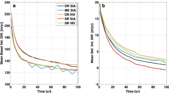
For a further analysis of the MarAsl2 velocity response with emphasis on upstream ice supply, we focus on the slid-ing area of Greenland below the 2000 m topographic contour. The resulting region provides the main supply for ice dis-charge at the marine margin. We additionally decompose the velocity field into its sliding component and the vertically averaged, deformational component (Fig. 8). Both compo-nents show an instant increase after the perturbation is ap-plied, which on average is about 250 m yr−1for sliding and 17 m yr−1for deformation. Yet the acceleration is attenuated fast in both components. The deformational component al-most completely returns to the reference value within one hundred years, while sliding remains at about 120 m yr−1 above the reference. Already the difference in magnitude highlights the importance of the sliding component for hor-izontal coupling. For the attenuation of the initial basal ac-celeration (Fig. 8a), it is striking that all model versions with horizontal coupling at the base (ME SIA, SR SIA, SR HO) group and show a more expressed dampening of the initial perturbation. An integration of this sliding perturbation over time would explain most of the model differences seen in the total mass loss (Fig. 2a). It seems only logical that for a perturbation in the sliding coefficient, it is the sliding veloc-ity that controls the response. Yet for the geometry perturba-tion in the MarCut experiment, this dominance is confirmed. It presumably results from our choice of the respective pa-rameters in the sliding law (Eq. B3) and the flow (Eq. A3). Also DR SIA and DR HO follow a similar sliding attenua-tion, which is not the case for their deformational component (Fig. 8b). Here model versions group according to the used deformational approximation with a weaker dampening for HO models. In essence, differences in ice deformation near the margin neither explain the spread in cumulative discharge (Fig. 2a) nor its magnitude. Dampened ice export thus results from faster attenuation of basal accelerations near the margin when including dynamic effects from horizontal gradients in membrane stresses.
4.4 Reaction times
Fig. 7.Decomposition of changes in ice discharge for MarAsl2 into contributions from different evolution in(a)ice thickness alone,(b) ve-locity magnitudes alone and(c)their combination (cf. Eq. 1). Together with changes in surface mass balance all these curves add up to the total volume loss in Fig. 2a.
each model version, each grid resolution, and each experi-ment into one scalar. We introduce a reaction time based on an exponential decay:
1D(t )=S·
1−exp(− t
τR
)
. (2)
The cumulative ice discharge1D has a saturation value S with a mean characteristic reaction time τR. The retrieved
values are averaged over one century. In this way informa-tion from the entire mass evoluinforma-tion enters the two parame-ters. The resultant mean reaction time shows magnitudes of several decades for marginal forcing (cf. Fig. 9) but it ex-ceeds hundreds of years for the TotAsl2 perturbation exper-iment. Therefore, we focus on the marginal forcing experi-ments with clear attenuation within our centennial scope.
A common characteristic for all margin perturbation ex-periments is the reduction of the reaction time when direct horizontal coupling is included in the basal layer (Fig. 9). The reason is that the instant velocity response exceeds the area of direct perturbation and thus allows geometric adjustment in a wider area than in DR SIA, resulting in faster attenua-tion. However, differences due to the model versions remain within 10 % of the DR SIA reference. Reaction time differ-ences between the model with a linearised effect of mem-brane stress gradients in the sliding law and the one account-ing for their full nonlinear impact (empty circles, Fig. 9a) are of the same order as those between other model versions. Therefore their linearisation (cf. Appendix B) is acceptable when the interest is in the centennial volume response. Yet the response behaviour is sensitive to the chosen grid res-olution and reaction times vary by up to 40 %. For both marginal perturbation experiments, reducing the grid resolu-tion lowers the reacresolu-tion time. This would be an undesirable effect if it simply arose from pure grid size reduction. For
this reason we repeated all experiments by simply supersam-pling the 20 km bed topography for the spin-up without using the detailed information from a higher resolution. Then the MarAsl2 set of experiments (not shown) has reaction times of about 40 yr with no monotone dependence on grid resolution. Consequently, the reduced reaction time in our experiments arises from additional information in the input data, which interfere with the spin-up and in turn affect the experimental setup. This behaviour is indeed a wanted effect because in re-ality geometries are complex and will affect the inland prop-agation of marginal perturbations. The MarCut experiment however shows the grid dependent reduction of the reaction time in both setups. Here this is a relict from an experimental setup disturbed by grid spacing. While MarAsl2 prescribes a constant 40 km extent of the sliding factor increase, the Mar-Cut perturbation has a direct effect only on the first grounded grid point upstream of the calving points. In summary, a con-sistent picture emerges for all marginal forcing experiments and for each resolution. Ice sheet reaction times are reduced when direct horizontal coupling operates and therefore al-low for a faster attenuation of marginal perturbations. Yet on a century timescale, this faster attenuation does not play a large role for the total mass loss of the GrIS.
5 Discussion
J. J. F ¨urst et al.: Effects of higher-order stress gradients 193
Fig. 8.Spatially averaged velocity response in MarAsl2 for the marginal sliding region decomposed into its basal(a)and mean deformational component(b). Background velocities from an unforced control experiment are subtracted. Due to changes in the extent of the sliding area, both velocity components were smoothed using a 5 yr running mean.
one is that the glaciostatic approximation neglects bridging effects in the vertical force balance. In addition, horizontal gradients in the vertical velocity field are assumed to be neg-ligible compared to vertical gradients in horizontal velocities. One might question whether these two assumptions result in a substantial loss in dynamic complexity that might inhibit important feedbacks for the transient ice sheet behaviour. Based on a scaling from an asymptotic analysis, Schoof and Hindmarsh (2010) present arguments that affirm the appli-cability of an LMLa model for large aspect ratios. The hor-izontal component of the LMLa velocity solution shows an error of second order in this ratio. Since the GrIS extent is at least two orders of magnitude larger than its thickness and since the horizontal grid spacing exceeds the ice thick-ness, our large-scale ice sheet model remains an appropri-ate tool for ice dynamics. Although Schoof and Hindmarsh (2010) emphasise the validity of the LMLa approach for slip and non-slip areas separately, the general scaling arguments might be violated in the transition zone (Schoof, 2006). How-ever, the higher-order LMLa approach is valid for dynamics in the vicinity of the ice divide where the nonlinearity of the viscous material causes a unique internal layer architecture, the Raymond effect (Raymond, 1983). In general, an LMLa model seems a feasible tool for transient, large-scale appli-cations and it is assumed that additional feedbacks in the FS equations are limited to smaller scales (<1 km) when stress regimes are well resolved.
Another issue concerns the poorly constrained sliding mechanisms beneath large-scale ice sheets (Fowler, 2010). Since the focus is on inland signal propagation, the applied sliding law should be capable of realistically transmitting margin perturbations upstream. Observations on Rutford Ice
Stream (Gudmundsson, 2011) suggest that a nonlinear mech-anism is a prerequisite to explain the upstream ice response to tidal forcing of different frequencies. A Weertman sliding law with an exponent of three reasonably explains the ob-served response pattern. This justifies its use for assessing the influence of direct horizontal coupling on inland signal transmission in the presented experimental framework.
At a numerical level, our choice for three distinct grid res-olutions alters and potentially inhibits direct horizontal cou-pling. Since we do not find a strong grid dependence of the total mass loss, it remains possible that direct horizontal cou-pling is not resolved properly on any used resolution. How-ever, on a 5 km grid, the initial speed-up in a 40 km vicinity (Fig. 4) is resolved and in agreement with theoretical esti-mates (Kamb and Echelmeyer, 1986). We are therefore con-vinced that membrane stress activity is captured in an accept-able way in our large-scale ice flow model. Except for resolv-ing successively more geometric details, we do not expect that further grid refinement would drastically alter model dif-ferences in the spatially integrated mass loss for these experi-ments. Underlining the consistency of our results, all of them are robust under different initial conditions (Fig. 2b).
Fig. 9.Mean reaction time retrieved for each experiment:(a)MarAsl2 and(b)MarCut. The dot sizes indicate the resolution on which the experiment was conducted. The largest and smallest dot size represents the 5 and 20 km grid, respectively. Reaction times are calculated based on Eq. (2). This timescale reflects the immediate response to a stepwise perturbation rather than a full ice sheet equilibration of many thousands of years.
spatial extent, the duration and the magnitude of the amplifi-cation in TotAsl2 exceed recent observations by far (McFad-den et al., 2011; Sundal et al., 2011). A simultaneous speed-up is also imposed for MarCut. From the three experiments this is the most severe one, with an equivalent sea level con-tribution that exceeds 100 mm. The other two experiments result in 45 mm and 16 mm after 100 yr. Though each ex-perimental perturbation is physically extreme, the resulting sea level contribution is in a realistic range with respect to present estimates for the increase in ice discharge rates (van den Broeke et al., 2009; Rignot et al., 2011). The reason is a fast attenuation of the initial perturbation and the conse-quently reduced centennial response. Therefore these exper-iments should be judged from the projected volume response rather than from the applied physical perturbation. The mod-elled mass loss range also agrees with other studies on dy-namic response of the GrIS (Price et al., 2011; Graversen et al., 2010). Graversen et al. (2010) conducted future projec-tions under various climate scenarios, parameterising a dou-bling of sliding speeds around Greenland. The resulting mass loss in these projections does not exceed 17 cm by the end of the 21st century, including uncertainties from the climate model ensemble. In their study, 15 % or 25 mm of the to-tal mass loss are associated with outlet glacier accelerations, which is somewhat lower than in TotAsl2. The reason for this is the imposed future warming that causes additional surface melt near the margin, where it removes the ice before it can reach the marine margin for calving.
6 Conclusion
A thermo-mechanically coupled 3-D large-scale ice sheet model with five versions of dynamic complexity was used to assess the influence of membrane stress gradients on the
centennial response of the GrIS under various marginal per-turbations. Results indicate that the SIA, which does not in-clude effects from direct horizontal coupling, already cap-tures the major response characteristics. In fact, the inclu-sion of membrane stress gradients actually reduces the vol-ume loss by up to 20 %. The reason is a faster attenuation of these perturbations by instant upstream accelerations and successive geometric adjustments. Including direct horizon-tal coupling also increases the area of direct influence. Our results exclude a dominant feedback between surface eleva-tion changes and surface mass balance; it is rather the ice dis-charge that abates more quickly and prevents sustained mass loss rates. The discharge reduction is moreover not explica-ble by additional marginal thinning but rather by faster atten-uation of the speed-up signal. Furthermore, the experiments have identified sliding as the component that reacts fastest and explains the differences in mass evolution. In summary, non-local effects from membrane stresses allow for a faster readjustment and attenuation of margin perturbations. Yet the general response of all model versions is similar to DR SIA, where signal transmission is accomplished by thickness dif-fusion alone.
An analysis of all experiments, model versions and grid resolutions shows that the reaction timescale is primarily de-pendent on the applied perturbation. The stronger the pertur-bation and the larger its spatial extent, the longer the reaction time. Putting aside the resolution dependence, the reaction time decreases by not more than 10 % when including direct horizontal coupling. This underlines the small effect of the dynamic complexity on the centennial volume evolution of the GrIS.
J. J. F ¨urst et al.: Effects of higher-order stress gradients 195
is in the volume evolution of an ice sheet, the classical SIA approach is sufficient to capture the main characteris-tics of the inland response. The higher-order approach SR HO is dynamically more complete but the additional com-putational cost (factor very dependent on chosen accuracies but in our case about 100) is not warranted by the limited gain in ice sheet volume response. A compromise could be the ME SIA approach (Bueler and Brown, 2009) with direct horizontal coupling at the base only. This approach is com-putationally much more efficient than SR HO (factor 20). Since basal velocity adjustment controls the signal attenu-ation ME SIA seems more appropriate than DR HO, though computationally they are comparable. When SR HO or FS models become computationally too expensive for a specific setup, we recommend the use of an ME SIA equivalent ap-proach (Hindmarsh, 2006; Bueler and Brown, 2009; Schoof and Hindmarsh, 2010).
In summary, differences in inland propagation of margin perturbations due to the degree of simplification of the force balance affect the ice sheet volume response only marginally. A self-accelerating dynamic feedback that would facilitate interior drainage and ultimately could trigger ice sheet disin-tegration is not confirmed. In addition, all perturbation exper-iments have a rather extreme character but the resulting mass loss is very limited. Simultaneous speed doubling all along the marine margin or in the entire sliding area goes far be-yond observed changes during the last decade. This strength-ens the view that the dominant effect on volume change of the Greenland ice sheet for the 21st century will come from sur-face mass balance changes. The largest source of uncertainty for future projections of ice sheets therefore arises from the climatic projections used as input rather than from the com-plexity of the ice-dynamic model.
Appendix A
Variants for ice deformation and basal resistance
A1 Ice deformation
Our glacial system is placed into an orthogonal coordinate system with three unit vectors {ex,ey,ez} in respectively horizontalx-,y- and verticalz-direction. The vertical axis of our coordinate system is chosen to be perpendicular to isolines of the gravitational field. In essence ice deformation is based on two balance equations for mass and momentum combined with a constitutive relation that links the stress tensorσ to strain rates and ultimately to the velocity field u=(ux,uy,uz). Considering an incompressible ice body, the balance equations take the following form:
∇ ·σ = −ρgez (A1)
∇ ·u=0 (A2)
Here, the gravitational accelerationgand the ice densityρ
are assumed constant (respective values are provided in Ta-ble 1). Ice creep is controlled by deviations from cryostatic pressure (τkl=σkl−13δklP
m
σmmwithk, l, m∈ {x, y, z})
rather than by the mean pressure itself. A simple power law is used to relate deviatoric stresses to strain ratesεfor poly-crystalline ice.
τkl=2ηε˙kl (A3)
η =1
2A T
•−1n ˙
ε 1−n
n
e (A4)
˙
ε2e =1
2 X
k,l ˙
εklε˙kl withk, l ∈ {x, y, z} (A5)
This constitutive equation is often referred to as Glen’s flow law while the effective viscosity η comprises the nonlinear dependence in the system because it itself de-pends on the effective strain rate ε˙e, a combination of all strain componentsε˙kl=12(∂lvk+∂kvl). The dependence on pressure melting point-corrected temperature T• of the rate factor follows an Arrhenius type function A (T•)=
A1/2exp(−B1/2/(RT•)) using two parameter sets for
dif-ferent temperature regimes. The rate factor also shows an age dependence since Wisconsin ice is assumed to deform more readily than Holocene ice for similar stress and tem-perature conditions. This rheologic influence of the ice age is described in Huybrechts (1994).
Our model offers the possibility to choose between two approximations for solving the Full Stokes (FS) equations (Eqs. A1, A2 and A3). The first is the shallow ice approxi-mation (SIA), which is standard practice in modelling large-scale ice sheets. In this approximation any influence from membrane stresses (as defined in Sect. 2.1) is neglected, which results in a balance between driving stress and vertical plane shearing.
∂iτiz=ρg∂is withi, j ∈ {x, y} (A6)
Heres indicates the surface elevation. Optionally we can determine the stress and velocity field by switching to a higher-order variant (HO) specified as LMLa (Hindmarsh, 2004; Schoof and Hindmarsh, 2010; Dukowicz et al., 2010). In this approximation of the force balance, horizontal varia-tions in lateral vertical shearing are negligible in the vertical balance Eq. (A1). In other words, the ice overburden pres-sure is locally compensated, meaning that any bridging ef-fects supporting ice weight sideways are comparably small.
˙
εiz=
1
2∂zui (A8)
This variant of a higher-order model holds a second sim-plification that makes the force balance independent of ver-tical velocities and thus allows to solely solve for the hor-izontal components. This decoupling becomes possible by considering horizontal gradients in the vertical velocity field, small compared to vertical gradients in the horizontal com-ponents∂ivz≪∂zvi (cf. Eq. A8). The vertical velocity com-ponent is in turn determined by mass conservation, i.e. in-compressibility (Eq. A2). As lateral boundary conditions to this force balance, ice thicknesses and velocity components are set to zero.
A2 Basal resistance
Ice deformation from SIA and HO are completed by three op-tions to determine the basal resistance (see Table 2). In gen-eral the basal resistanceτbicompensates effects from vertical plane shearing and stress transmitted by membrane stresses.
τb||i=τiz(b)−2τii(b)+τjj(b)∂ib−τij(b)∂jb (A9)
fori6=j andi, j∈ {x, y} Here sub- and superscriptbindicate that stress terms have to be evaluated at bed elevation (z=b).τb||iis the stress com-ponent parallel to the bed surface. A first option for basal re-sistance arises from assumptions made for the SIA. Neglect-ing effects from membrane stresses, basal drag is balanced by vertical plane shearing at the base, which equals the driving stressτd.
τb||i=τdi =ρgH ∂is (A10)
Calculating the basal drag in this way is referred to as the driving stress (DR) option. In contrast to this dominance of vertical plane shearing at the base is an approach that high-lights the importance of membrane stresses. It stems from assuming a vertically uniform stress and velocity field, thus without vertical plane shearing, while the whole setup is bal-anced by membrane stresses. In analogy to Bueler and Brown (2009) and using identical frictional forcing at the ice surface and at its base, the resulting force balance is used to deter-mine the basal stress field.
τb||i=ρgH ∂is−∂i
2H τiiSSA, b+H τjjSSA, b (A11) −∂j
H τijSSA, b fori6=j τijSSA =2ηSSAε˙SSAij
ηSSA =1
2A T
•−1n ˙
εSSAe − 1−n
n
˙
εSSAe 2=1
2 X
ij ˙
εSSAij ε˙SSAij
This resistance option with dominant membrane stresses (ME) resembles a shallow shelf approximation (SSA) apart that for our purpose it serves to determine the condition for the frictional basal boundary. As a result from vertical in-tegration the effective viscosity ηSSA is purely determined by horizontal strains that control the evolution of a float-ing shelf. In analogy to the HO ice deformation, a last op-tion arises from neglecting horizontal gradients in the verti-cal velocity field for the strain rates. As a consequence a HO version of the resistance Eq. (A9) is obtained. This way of balancing the basal drag uses a slightly simplified resistance (SR) equation and is referred to as SR option. Together with two options for ice deformation, this gives six versions of treating basal resistance and deformation in our model (see Table 2).
Appendix B
Boundary conditions
In order to find a unique solution for Eqs. (A1), (A2) and (A3), boundary conditions are required. At the ice-free points around the lateral boundary we set not only the ice thick-ness H to zero but also the velocity field. This Dirichlet boundary condition is widely used in ice sheet modelling al-though resulting margin gradients are in essence dictated by grid spacing. For the vertical boundaries, conditions become more elaborate.
B1 Free surface
The upper surface boundary condition is set up in a similar way as the one for the base Eq. (A9) except that it must be evaluated at surface elevation (z=s).
τs||i=τiz(s)−2τii(s)+τjj(s)∂is−τij(s)∂js (B1)
fori6=j andi, j∈ {x, y} However, since the contact with the atmosphere does not pro-vide any resistance to the ice flow, its drag is zero, imposing an internal balance of stresses at the ice surface.
τs||i=0 (B2)
Note that for the SIA this relation is automatically fulfilled since vertical shearing becomes zero at the upper boundary.
B2 Basal sliding
J. J. F ¨urst et al.: Effects of higher-order stress gradients 197
sliding is controlled by regelation, enhanced creep, effective water pressure, bedrock roughness and cavitation geometry (Fowler, 2010; Schoof, 2005, 2010). When ice overlays a till layer, finding an appropriate sliding relation becomes more elaborate since a reasonable rheology for till must be formu-lated. As a granular material with a yield stress, observations confirm that till is well described assuming a plastic rheol-ogy (e.g. Tulaczyk, 2000). However, field measurements on Iceland (Boulton and Hindmarsh, 1987) indicate a nonlinear viscous rheology with an exponent of three (m=3). Such a nonlinear mechanism was found to be a prerequisite for re-alistic inland transmission of tidal forcing in Antarctic ice streams (Gudmundsson, 2011).
τbi =C Hmu
1−m m
b ubi m
ubi =
Asl
H τ
m−1
b τbi withi∈ {x, y}(B3) m
Hβ2ubi=τbmi
C−
1
m=Asl=β−2 (B4)
Hereubis the basal velocity magnitude andubi each vec-tor component. In the literature, this viscous approach is ex-pressed either in a nonlinear basal friction equation or a non-linear sliding relation.C is the friction parameter, whileβ2
is the friction coefficient and both are inversely related to the basal sliding coefficientAsl. An enhancement of sliding
to-wards the ice sheet margin is introduced by a weighting of the coefficients with ice thickness. Equation (B3) together with Eq. (A9) allow for a solution of the partial differential Eqs. (A1), (A2) and (A3) uniquely. However for practical reasons a partially linearised sliding relation is introduced.
ubi=
Asl
H τ
m−1
d τbi (B5)
Here the nonlinearity of the sliding relation is accounted for by the driving stress τd, which is fully prescribed by
the ice geometry. This leaves a linear relation between basal velocitiesuband basal dragτbwith a highly geometry de-pendent proportionality factor. Our linear solver can directly handle such a linear sliding relation. In order to solve the full nonlinear Eq. (B3) an iterative method is chosen that con-secutively updatesτbuntil convergence is reached (for more
details see analogue viscosity update described in F¨urst et al., 2011).
Acknowledgements. This research received funding from the ice2sea programme from the European Union 7th Framework Programme grant number 226375, the Research Foundation – Flanders (FWO) project NEEM-B, and the Belgian Federal Science Policy Office within its Research Programme on Science for a
Sustainable Development under contract SD/CS/06A (iCLIPS). This publication has the ice2sea contribution number 131.
Edited by: E. Larour
References
Amundson, J. M., Fahnestock, M., Truffer, M., Brown, J., Luthi, M. P., and Motyka, R. J.: Ice melange dynamics and implications for terminus stability, Jakobshavn Isbrae Greenland, J. Geophys. Res.-Earth, 115, F01005, doi:10.1029/2009JF001405, 2010. Bamber, J. L., Layberry, R. L., and Gogineni, S. P.: A new ice
thick-ness, bed dataset for the Greenland ice sheet 1; Measurement, data reduction, and errors, J. Geophys. Res.-Atmos., 106, 33773– 33780, doi:10.1029/2001JD900054, 2001.
Bartholomew, I., Nienow, P., Mair, D., Hubbard, A., King, M. A., and Sole, A.: Seasonal evolution of subglacial drainage and ac-celeration in a Greenland outlet glacier, Nat. Geosci., 3, 408–411, doi:10.1038/NGEO863, 2010.
Benn, D. I., Warren, C. R., and Mottram, R. H.: Calving processes and the dynamics of calving glaciers, Earth-Sci. Rev., 82, 143– 179, doi:10.1016/j.earscirev.2007.02.002, 2007.
Boulton, G. S. and Hindmarsh, R. C. A.: Sediment Deformation beneath Glaciers: Rheology and geological consequences, J. Geophys. Res., 92, 9059–9082, doi:10.1029/JB092iB09p09059, 1987.
Briner, J. P., Bini, A. C., and Anderson, R. S.: Rapid early Holocene retreat of a Laurentide outlet glacier through an Arctic fjord, Nat. Geosci., 2, 496–499, doi:10.1038/ngeo556, 2009.
Bueler, E. and Brown, J.: Shallow shelf approximation as a “sliding law” in a thermomechanically coupled ice sheet model, J. Geo-phys. Res., 114, F03008, doi:10.1029/2008JF001179, 2009. Christoffersen, P., Mugford, R. I., Heywood, K. J., Joughin, I.,
Dowdeswell, J. A., Syvitski, J. P. M., Luckman, A., and Ben-ham, T. J.: Warming of waters in an East Greenland fjord prior to glacier retreat: mechanisms and connection to large-scale atmo-spheric conditions, The Cryosphere, 5, 701–714, doi:10.5194/tc-5-701-2011, 2011.
Dukowicz, J. K., Price, S. F., and Lipscomb, W. H.: Consistent approximations and boundary conditions for ice-sheet dynam-ics from a principle of least action, J. Glaciol., 56, 480–496, doi:10.3189/002214310792447851, 2010.
Fowler, A. C.: Weertman, Lliboutry and the develop-ment of sliding theory, J. Glaciol., 56, 965–972, doi:10.3189/002214311796406112, 2010.
F¨urst, J. J., Rybak, O., Goelzer, H., De Smedt, B., de Groen, P., and Huybrechts, P.: Improved convergence and stability properties in a three-dimensional higher-order ice sheet model, Geosci. Model Dev., 4, 1133–1149, doi:10.5194/gmd-4-1133-2011, 2011. Graversen, R. G., Drijfhout, S., Hazeleger, W., van de Wal, R.,
Bin-tanja, R., and Helsen, M.: Greenland’s contribution to global sea-level rise by the end of the 21st century, Clim. Dynam., 37, 1427– 1442, doi:10.1007/s00382-010-0918-8, 2010.
Gudmundsson, G. H.: Ice-stream response to ocean tides and the form of the basal sliding law, The Cryosphere, 5, 259–270, doi:10.5194/tc-5-259-2011, 2011.
Hindmarsh, R. C. A.: The role of membrane-like stresses in deter-mining the stability and sensitivity of the Antarctic ice sheets: back pressure and grounding line motion, Philos. T. Roy. Soc. A., 364, 1733–1767, doi:10.1098/rsta.2006.1797, 2006. Holland, D. M., Thomas, R. H., De Young, B., Ribergaard, M. H.,
and Lyberth, B.: Acceleration of Jakobshavn Isbrae triggered by warm subsurface ocean waters, Nat. Geosci., 1, 659–664, doi:10.1038/ngeo316, 2008.
Howat, I. M. and Eddy, A.: Multi-decadal retreat of Green-land’s marine-terminating glaciers, J. Glaciol., 57, 389–396, doi:10.3189/002214311796905631, 2011.
Howat, I. M., Joughin, I., Fahnestock, M., Smith, B. E., and Scambos, T. A.: Synchronous retreat and acceleration of southeast Greenland outlet glaciers 2000–06: ice dy-namics and coupling to climate, J. Glaciol., 54, 646–660, doi:10.3189/002214308786570908, 2008.
Howat, I. M., Box, J. E., Ahn, Y., Herrington, A., and McFad-den, E. M.: Seasonal variability in the dynamics of marine-terminating outlet glaciers in Greenland, J. Glaciol., 56, 601– 613, doi:10.3189/002214310793146232, 2010.
Hutter, K.: Theoretical Glaciology; material science of ice and the mechanics of glaciers and ice sheets, D. Reidel Publishing Com-pany/Tokyo, Terra Scientific Publishing Company, Dordrecht, Boston, Tokyo, Japan, and Hingham, MA, ISBN 9027714738, 1983.
Huybrechts, P.: The present evolution of the Greenland ice sheet – An assessment By Modelling, Global Planet. Change, 9, 39–51, doi:10.1016/0921-8181(94)90006-X, 1994.
Huybrechts, P.: Sea-level changes at the LGM from ice-dynamic reconstructions of the Greenland and Antarctic ice sheets dur-ing the glacial cycles, Quaternary Sci. Rev., 21, 203–231, doi:10.1016/S0277-3791(01)00082-8, 2002.
Huybrechts, P. and de Wolde, J.: The dynamic response of the Greenland and Antarctic ice sheets to multiple-century cli-matic warming, J. Climate, 12, 2169–2188, doi:10.1175/1520-0442(1999)012¡2169:TDROTG¿2.0.CO;2, 1999.
Huybrechts, P., Goelzer, H., Janssens, I., Driesschaert, E., Fichefet, T., Goosse, H., and Loutre, M.-F.: Response of the Greenland and Antarctic Ice Sheets to Multi-Millennial Greenhouse Warming in the Earth System Model of Intermediate Complexity LOVE-CLIM, Surv. Geophys., 32, 397–416, doi:10.1007/s10712-011-9131-5, 2011.
Joughin, I., Howat, I. M., Fahnestock, M., Smith, B., Krabill, W., Alley, R. B., Stern, H., and Truffer, M.: Continued evolution of Jakobshavn Isbrae following its rapid speedup, J. Geophys. Res., 113, F04006, doi:10.1029/2008JF001023, 2008.
Joughin, I., Smith, B. E., Howat, I. M., Scambos, T., and Moon, T.: Greenland flow variability from ice-sheet-wide velocity mapping, J. Glaciol., 56, 415–430, doi:10.3189/002214310792447734, 2010.
Jouvet, G., Huss, M., Blatter, H., Picasso, M., and Rappaz, J.: Numerical simulation of Rhonegletscher from 1824 to 2100, J. Comput. Phys., 228, 6426–6439, doi:10.1016/j.jcp.2009.05.033, 2009.
Kamb, B. and Echelmeyer, K. A.: Stress-Gradient Coupling Glacier Flow. 1. Longitudinal Averaging of the Influence of Ice Thick-ness and Surface Slope, J. Glaciol., 32, 267–284, 1986. Luthcke, S. B., Zwally, H. J., Abdalati, W., Rowlands, D. D.,
Ray, R. D., Nerem, R. S., Lemoine, F. G. McCarthy, J. J., and
Chinn, D. S.: Recent Greenland ice mass loss by drainage system from satellite gravity observations, Science, 314, 1286–1289, doi:10.3189/002214308784886117, 2006.
McFadden, E. M., Howat, I. M., Joughin, I., Smith, B., and Ahn, Y.: Changes in the dynamics of marine terminating outlet glaciers in west Greenland (2000–2009), J. Geophys. Res., 116, F02022, doi:10.1029/2010JF001757, 2011.
Moon, T., Joughin, I., Smith, B., and Howat, I.: 21st-Century Evo-lution of Greenland Outlet Glacier Velocities, Science, 336, 576– 578, doi:10.1126/science.1219985, 2012.
Motyka, R. J., Truffer, M., Fahnestock, M., Mortensen, J., Rysgaard, S., and Howat, I.: Submarine melting of the 1985 Jakobshavn Isbrae floating tongue and the trigger-ing of the current retreat, J. Geophys. Res., 116, F01007, doi:10.1029/2009JF001632, 2011.
Nick, F. M., Vieli, A., Howat, I. M., and Joughin, I.: Large-scale changes in Greenland outlet glacier dynamics triggered at the ter-minus, Nat. Geosci., 2, 110–114, doi:10.1038/NGEO394, 2009. Nick, F. M., van der Veen, C. J., Vieli, A., and Benn, D. I.: A
phys-ically based calving model applied to marine outlet glaciers and implications for the glacier dynamics, J. Glaciol., 56, 781–794, doi:10.3189/002214310794457344, 2010.
Pattyn, F.: A new three-dimensional higher-order thermomechani-cal ice sheet model: Basic sensitivity, ice stream development, and ice flow across subglacial lakes, J. Geophys. Res.-Sol. Ea., 108, 1–15, doi:10.1029/2002JB002329, 2003.
Phillips, T., Rajaram, H., and Steffen, K.: Cryo-hydrologic warming: A potential mechanism for rapid thermal re-sponse of ice sheets, Geophys. Res. Lett., 37, L20503, doi:10.1029/2010GL044397, 2010.
Price, S. F., Payne, A. J., Catania, G. A., and Neumann, T. A.: Seasonal acceleration of inland ice via longitudinal coupling to marginal ice, J. Glaciol., 54, 213–219, 2008.
Price, S. F., Payne, A. J., Howat, I. M., and Smith, B.: Commit-ted sea-level rise for the next century from Greenland ice sheet dynamics during the past decade, P. Natl. Acad. Sci. USA, 108, 8978–8983, doi:10.1073/pnas.1017313108, 2011.
Raymond, C. F.: Deformation in the vicinity of ice divides, J. Glaciol., 29, 357–373, 1983.
Rignot, E., Velicogna, I., van den Broeke, M. R., Monaghan, A., and Lenaerts, J.: Acceleration of the contribution of the Greenland and Antarctic ice sheets to sea level rise, Geophys. Res. Lett., 38, L05503, doi:10.1029/2011GL046583, 2011.
Ritz, C., Rommelaere, V., and Dumas, C.: Modeling the evolution of Antarctic ice sheet over the last 420,000 years: Implications for altitude changes in the Vostok region, J. Geophys. Res.-Atmos., 106, 31943–31964, doi:10.1029/2001JD900232, 2001.
Sasgen, I., van den Broeke, M., Bamber, J. L., Rignot, E., Sørensen, L. S., Wouters, B., Martinec, Z., Velicogna, I., and Simon-sen, S. B.: Timing and origin of recent regional ice-mass loss in Greenland, Earth Planet. Sc. Lett., 333–334, 393–303, doi:10.1016/j.epsl.2012.03.033, 2012.
Scambos, T. A., Hulbe, C., Fahnestock, M., and Bohlander, J.: The link between climate warming and break-up of ice shelves in the Antarctic Peninsula, J. Glaciol., 46, 516–530, doi:10.3189/172756500781833043, 2000.
J. J. F ¨urst et al.: Effects of higher-order stress gradients 199
Schoof, C.: A variational approach to ice streams flow, J. Fluid. Mech., 556, 227–251, doi:10.1017/S0022112006009591, 2006. Schoof, C.: Ice sheet grounding line dynamics: Steady states,
stability, and hysteresis, J. Geophys. Res., 112, F03S28, doi:10.1029/2006JF000664, 2007.
Schoof, C.: Ice-sheet acceleration driven by melt supply variability, Nature, 468, 803–806, doi:10.1038/nature09618, 2010. Schoof, C. and Hindmarsh, R. C. A.: Thin-Film Flows with
Wall Slip: An Asymptotic Analysis of Higher Order Glacier Flow Models, Q. J. Mech. Appl. Math., 63, 73–114, doi:10.1093/qjmam/hbp025, 2010.
Schrama, E. J. O. and Wouters, B.: Revisiting Greenland ice sheet mass loss observed by GRACE, J. Geophys. Res., 116, B02407, doi:10.1029/2009JB006847, 2011.
Seddik, H., Greve, R., Zwinger, R., Gillet-Chaulet, F., and Gagliar-dini, O.: Simulations of the Greenland ice sheet 100 years into the future with the full Stokes model Elmer/Ice, J. Glaciol., 58, 448–456, doi:10.3189/2012JoG11J177, 2012.
Slobbe, D. C., Lindenbergh, R. C., and Ditmar, P.: Estimation of volume change rates of Greenland’s ice sheet from ICESat data using overlapping footprints, Remote Sens. Environ., 112, 4204– 4213, doi:10.1016/j.rse.2008.07.004, 2008.
Sørensen, L. S., Simonsen, S. B., Nielsen, K., Lucas-Picher, P., Spada, G., Adalgeirsdottir, G., Forsberg, R., and Hvidberg, C. S.: Mass balance of the Greenland ice sheet (2003–2008) from ICE-Sat data – the impact of interpolation, sampling and firn density, The Cryosphere, 5, 173–186, doi:10.5194/tc-5-173-2011, 2011. Straneo, F., Hamilton, G. S., Sutherland, D. A., Stearns, L. A.,
Davidson, F., Hammill, M. O., Stenson, G. B., and Rosing-Asvid, A.: Rapid circulation of warm subtropical waters in a major glacial fjord in East Greenland, Nat. Geosci., 3, 182–186, doi:10.1038/NGEO764, 2010.
Straneo, F., Curry, R. G., Sutherland, D. A., Hamilton, G. S., Cenedese, C., Vage, K., and Stearns, L. A.: Impact of fjord dynamics and glacial runoff on the circulation near Helheim Glacier, Nat. Geosci., 4, 322–327, doi:10.1038/NGEO1109, 2011.
Sundal, A. V., Sheperd, A., Nienow, P., Hanna, E., Palmer, S., and Huybrechts, P.: Melt-induced speed-up of Greenland ice sheet offset by efficient subglacial drainage, Nature, 469, 521–524, doi:10.1038/nature09740, 2011.
Thomas, R., Frederick, E., Krabill, W., Manizade, S., and Martin, C.: Recent changes on Greenland outlet glaciers, J. Glaciol., 55, 147–162, doi:10.3189/002214309788608958, 2009.
Tulaczyk, S., Kamb, W. B., and Engelhardt, H. F.: Basal mechanics of Ice Stream B, West Antarctica 1. Till mechanics, J. Geophys. Res.-Sol. Ea., 463–481, 105, doi:10.1029/1999JB900329, 2000. van den Broeke, M. R., Bamber, J., Ettema, J., Rignot, E., Schrama, E., van de Berg, W.-J., van Meijgaard, E., Velicogna, I., and Wouters, B.: Partitioning Recent Greenland Mass Loss, Science, 326, 984–986, doi:10.1126/science.1178176, 2009.
Velicogna, I.: Increasing rates of ice mass loss from the Green-land and Antarctic ice sheets revealed by GRACE, Geophys. Res. Lett., 36, L19503, doi:10.1029/2009GL040222, 2009.
Williams, R., Hindmarsh, R. C. A., and Arthern, R. J.: Frequency response of ice streams, Proc. R. Soc. A., 468, 3285–3310, doi:10.1098/rspa.2012.0180, 2012.
Zwally, H. J., Abdalati, W., Herring, T., Larson, K., Saba, J., and Steffen, K.: Surface melt-induced acceleration of Greenland ice-sheet flow, Science, 297, 218–222, doi:10.1126/science.1072708, 2002.
Zwally, H. J., Giovinetto, M. B., Li, J., Cornejo, H. G., Beckley, M. A., Brenner, A. C., Saba, J. L., and Yi, D. H.: Mass changes of the Greenland and Antarctic ice sheets and shelves and con-tributions to sea-level rise: 1992–2002, J. Glaciol., 51, 509–527, doi:10.3189/172756505781829007, 2005.
Zwally, H. J., Li, J., Brenner, A. C., Beckley, M., Cornejo, H. G., Dimarzio, J., Giovinetto, M. B., Neumann, T. A., Robbins, J., Saba, J., Yi, D. H., and Wang, W. L.: Greenland ice sheet mass balance: distribution of increased mass loss with climate warming; 2003–07 versus 1992–2002, J. Glaciol., 57, 88–102, doi:10.3189/002214311795306682, 2011.