Mergers & acquisitions : Portucel and Suzano Papel e Celulose

(1)

Mergers & Acquisitions: Portucel and

Suzano Papel e Celulose

Master Thesis

Vitor Oliveira

Advisor: Peter Tsvetkov

September 2014

(2)

Acknowledgments

I would like to thank, in first place, to all his CLSBE teachers throughout the master, for their commitment in my continuous development. Secondly, I must thank the seminar advisor, Peter Tsvetkov, for its insightful comments on this thesis as well as for being constantly available, even throughout the summer. Also to my family, who have supported me through my life and were the main contributors to the little I’ve achieved. Many thanks to all my good friends and to Pedro Gancho and Ana Simões in particular. And finally, to Mariana, for being my best friend.

Abstract

The pulp and paper industry is, nowadays, facing challenges associated with the lack of demand growth, pushing firms to adapt to intense competition and industry-wide overcapacity. In order to remain profitable and achieve sustainable competitive positions, industry players have relied on M&A to achieve scale and expand into growing markets in emerging countries. The industry concentration conducted through mergers has been able to deliver value to shareholders while changing the overall competitive landscape.

This dissertation’s goal is to propose a merger between Suzano Papel e Celulose and Portucel. The proposition is supported by a review of the main literature on M&A, a thorough industry and company analysis, and a valuation of each individual firm and its combination.

It is concluded that Suzano should acquire Portucel in an all-stock offer, valuing the Portuguese firm at €4.32, a premium of 55% over its 31 December 2013 market capitalization. Through the proposed takeover offer, Portucel would be entitled to 46% of the merged firm, with the remaining 54% allocated to Suzano’s shareholders.

(3)

5.2. Portucel – Forecasts ... 54 5.2.1. Energy Revenues ... 54 5.2.2. Operational Costs ... 55 5.2.3. CAPEX ... 56 5.2.4. Depreciations ... 57 5.2.5. Working Capital ... 57 5.2.6. Debt ... 57 5.2.7. Dividends ... 57 5.3. Suzano – Forecasts ... 58 5.3.1. Revenues ... 58 5.3.2. Operational Costs ... 59 5.3.3. CAPEX ... 60 5.3.4. Depreciations ... 60 5.3.5. Working Capital ... 61

5.3.6. Debt and interest... 62

5.2.7. Dividends ... 63

6. Rationale for the proposed transaction ... 63

7. Standalone Valuation ... 66

7.1. Pro-forma financial statements ... 66

7.1.1. Portucel ... 66 7.1.2. Suzano ... 67 7.2. Cost of Capital ... 68 7.3. Valuation Models ... 70 7.3.1. Portucel ... 70 7.3.1.1. DCF ... 70

(6)

7.3.1.2. Dividend Discount Model ... 71 7.3.1.3. Sensitivity Analysis ... 72 7.3.2. Suzano ... 73 7.3.2.1. DCF ... 74 7.3.2.2. APV ... 75 7.3.2.3. Sensitivity Analysis ... 75

8. Recent comparable M&A deals... 76

9. The Merger ... 77

9.1. Valuation without Synergies ... 77

9.2. Synergies ... 78

9.2.1. Cost Synergies ... 78

9.2.2. Revenue Synergies ... 80

9.2.3. Financial Synergies ... 81

9.3. Integration Costs ... 83

9.4. Valuation of the merged firm ... 83

9.4.1. Synergy Valuation ... 84

9.4.2. Valuation accounting for the new project ... 85

9.4.3. Operating sense of synergies ... 85

9.5. The acquisition ... 86

9.5.1. Bidder and target definition ... 86

9.5.2. Distribution of the synergies ... 86

9.5.3. Method of payment ... 87

9.5.4. Takeover offer ... 88

9.5.5. SVAR ... 89

9.5.6. Other Potential Bidders ... 89

9.5.7. Execution Risk ... 90

10. Conclusion ... 91

11. Appendix ... 92

(7)

List of Figures

FIGURE 1: GLOBAL M&A VOLUME, BY YEAR. FIGURE 2: GLOBAL M&A BY SECTOR, 2014.

FIGURE 3: ENTERPRISE VALUE AND EBITA ADJUSTMENTS FIGURE 4: MEET THE PREMIUM LINE

FIGURE 5: CAPABILITIES/MARKET ACCESS FRAMEWORK. FIGURE 6: PULP AND PAPER INDEX PRICES

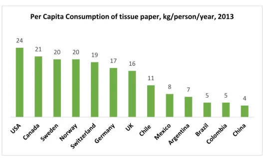
FIGURE 7: NUMBER OF MILLS AND TOTAL PULP PRODUCTION VOLUME IN EUROPE FIGURE 8: DEMAND OF PRINTING & WRITING PAPER BY REGION IN VOLUME FIGURE 9: PER CAPITA CONSUMPTION OF TISSUE PAPER

FIGURE 10: TOTAL REVENUES

FIGURE 11: INTEGRATED PAPER REVENUES

FIGURE 12: PAPER PRODUCTION, SALES AND CAPACITY IN VOLUME FIGURE 13: MARKET SHARE IN BRAZIL BY SEGMENT

FIGURE 14: TOP 10 PULP PRODUCERS FIGURE 15: PULP REVENUES

FIGURE 16: PULP PRODUCTION, SALES AND CAPACITY IN VOLUME FIGURE 17: PULP SALES BY GEOGRAPHIC SEGMENT

FIGURE 18: COGS

FIGURE 19: SALES EXPENSES

FIGURE 20: GENERAL AND ADMINISTRATIVE EXPENSES FIGURE 21: EBITDA

FIGURE 22: CAPITAL EXPENDITURES FIGURE 23: INTEREST-BEARING LIABILITIES FIGURE 24: TOTAL REVENUES

FIGURE 25: INTEGRATED PULP AND PAPER REVENUES FIGURE 26: PAPER REVENUES BY MARKET SEGMENT FIGURE 27: PULP REVENUES AND PULP PRICE INDEX FIGURE 28: TOTAL OPERATIONAL COSTS

(8)

FIGURE 30: OPERATIONAL PROFIT BY PRODUCT SEGMENT FIGURE 31: CAPITAL EXPENDITURES

FIGURE 32: TOTAL INTEREST-BEARING LIABILITIES FIGURE 33: PAPER, PULP AND MSCI WORLD INDEX

(9)

1. Introduction

In the online era we live in, where a rapid shift from paper to digital based content is observed, the paper industry is on the verge of reaching the decline stage. As the industry is highly correlated with economic environment, the global economic and financial crisis of 2008 has spurred a wave of bankruptcies, due to industry overcapacity and high leverage levels. Indeed, the structural problems the industry suffered due to stagnant or decreasing demand were deeply aggravated by the crisis. An industry restructuring phase ensued, which has lasted through to today. While some firms are able to be profitable and have sustainable leverage levels, others struggle to compete in current market conditions. Indeed, over the last years it has been proven that firms with industrial efficiency and scale struggle to be profitable, which has led to intense M&A activity in the industry, primarily to concentrate supply. Additionally, firms based in Europe and North America seek to expand to markets where growth rates are more attractive, typically in emerging countries, and often do so through acquisitions.

Suzano Papel e Celulose and Portucel, the two companies under scrutiny in this thesis, are part of and influenced by the abovementioned industry trends. Albeit quite distinct, the two firms share a few common characteristics: both have a strong regional presence in the paper industry and a global reach in their pulp segment and both are entering a new stage of their lifecycle. Suzano, a Brazilian based company, has plenty opportunities to expand organically but is unable to source the capital required to pursue those opportunities, having a highly leveraged capital structure. Portucel, on the contrary, seems to have reached the end of its previous growth model of developing highly efficient mills in Portugal. Without opportunities to deploy its constantly growing cash resources, the firm is not growing nor will it in the foreseeable future, under current conditions.

First, the applicable previous research on the various subjects discussed throughout the thesis is reviewed in the Literature Review section. Following the Literature Review, an industry analysis is conducted and an in-depth analysis of the two firms to be merged. Forecasts on the main indicators of future performance is discussed and detailed in the Forecasts section. Before the results of the valuation models are presented, the rationale for the proposed transaction is clearly explained. Both Suzano and Portucel are individually valued using two alternative valuation models, which are then compared and their key assumptions tested recurring to sensitivity analysis. After a review of recent comparable mergers which formed the basis to estimate synergies and integration costs, the last part of this thesis concerns the

(10)

estimated and integrated in the valuation of the merged firm. Finally, the structure of the deal, its risks and possible competition are discussed in The Acquisition section.

2. Literature Review

2.1. Recent trends in M&A

2.1.1 Cyclicality

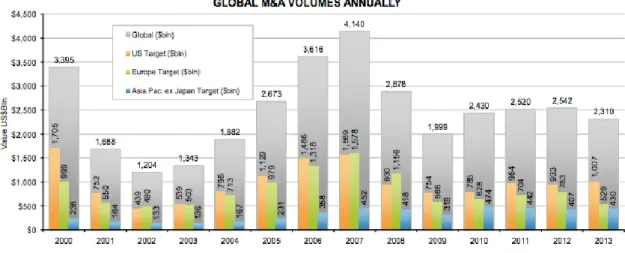
FIGURE 1: GLOBAL M&A VOLUME, BY YEAR. SOURCE: THOMSON REUTERS

M&A activity is cyclical, usually following a pattern of robust growth, eventually reaching a peak and initiating a downward path, usually sharp and simultaneously to an economic and/or financial slowdown (or a crisis). M&A activity is highly correlated with GDP growth and with the stock market. Therefore, a downturn in the economy leads to a decrease in the dollar volume of mergers and acquisitions.

The cyclicality feature of M&A can be observed from 2000 on (see Figure 1). After a peak in volume of $3.4 trillion in 2000, deals went sharply down to $1.2 trillion in 2002. Deals resurged in 2003 and M&A activity increased rapidly until 2007, reaching an all time high of $4.14 trillion. With the 2008 financial crisis and consequent global recession, the volume again plummeted, to $2 trillion. Subsequent years brought about a recovery which is still distant from 2007 values. In 2013, the global M&A volume reached $2.3 trillion, $200 billion less than 2012.

With the S&P 500 in its all time high and a bull market around the globe, a KPMG (2013) survey shows investors are confident regarding the current M&A environment and optimist for more deals, both in number and volume, in 2014. The investors surveyed use three corporate observations to justify their expectations - companies have accumulated large cash reserves,

(11)

better credit terms and are avid to exploit opportunities in emerging markets. In turn, yield starved investors are likely to push corporate managers to pursue deals to use excess cash rather than returning it as dividends.

2.1.2. Which stage of the cycle? M&A market in 2014- 2015

There was a general agreement that the year of 2013 would mark the return to higher levels of M&A, possibly reaching pre-crisis levels. However, total deal value for the year lagged 2007 levels by a great margin, failing to reach even the 2010 figure. The activity expected for 2013 is set to be observed in 2014. In the first months of 2014, deals amounted to $1.2 trillion, comparing to $1.4 trillion over the same period of 2007.

In hindsight, the M&A boom of 2007 proved to be unsustainable. The financial and economic crisis that ensued marked the end of a growth stage in the M&A cycle, and volumes plummeted to decade long lows. In 2014, with deal values again reaching pre-crisis figures, the title of this section is a question that begs an answer. To understand whether these figures will be sustainable is key to accurately predict if a peak is once again forming and another M&A market bust will follow.

Comparing the first four months of 2007 and 2014 beyond the similarity of total values shows that there has been a shift in the way deals are done (Hammond, 2014). A Delloite (2014) study highlights the key differences between deals in both periods. Before 2007, M&A deals generally meant high leverage levels, with companies borrowing to finance their acquisitions done entirely with cash as payment method (76% of deals were all-cash in the first four months of 2007). In 2014, although cash is still king, more than half the deals relied substantially in stock as a method of payment. Another stark difference in M&A from 2007 to 2014 concerns market perceptions. Indeed, the market perceives deals being done as more strategic and value-creating than before: bidder’s stock prices have since 2013 increased an average of 4.4% in the first day after announcement. This is quite a paradigm changing event – acquirers’ share prices drops when deals first come to public has been a constant throughout the history of M&A. Another important data point is the 30% rise in equity markets of 2013, compared with a stable M&A volume over the same period. Given the fact that both are highly correlated, the M&A volume surge in 2014 can be but a mean-reverting process, according to Bob Eatroff, head of M&A at Morgan Stanley US. All in all, although the recent trend formed in the beginning of 2014 closely mimics the trend before the crisis, the fact that the type of deals

(12)

have changed doesn’t allow for the conclusion that a peak has been reached and the cycle will turn south in the near future.

In terms of M&A activity by sector, telecoms, healthcare, technology and real-estate sectors dominate in terms of weight in total value, together accounting for 52% of total value, in 2014. The sector with the larger share of value was telecommunications, with deals amounting to $252 billion in the first four months of 2014. Other sectors with relevant weight are Oil&Gas (6%), Construction (5%) and Finance (5%). Other sectors compose a third of global value.

FIGURE 2: GLOBAL M&A BY SECTOR, 2014. SOURCE: FINANCIAL TIMES

2.1.2 Cross-border M&A activity

M&A is still mainly done domestically, both in developed and emerging countries. However, cross-border deals are increasingly popular, especially for mature firms which rely on acquisitions to enter new markets. In a Grant Thornton (2013) study, a third of the surveyed firms plan to make an overseas acquisition in the next three years, with nearly half of the European based firms planning to engage in cross-border M&A in the short-term future. Cross-border and domestic mergers alike happen for the same reason: to the acquirers, the combined entity is more valuable than they are worth separately. However, it is widely agreed that cross-border M&A is usually more challenging and complex. The added complexity arises from cultural and geographic differences and its adverse impact on the integration process as well as the imperfect integration of capital markets, namely in stock and currency markets (Erel, Liao and Weisbach, 2010). This makes acquirers struggle to deliver expected value from

(13)

their acquisitions abroad: a KPMG (1999) study finds that only 17% of cross-border M&A deals created shareholder value.

A key issue in cross-border deal activity is the corporate governance standards in of target firms. Cross-border deals are done in a stock swap when the acquirer’s country shows better governance, shareholder protection and transparency. The acquirer’s lower governance risk increases the attractiveness of its stock for the shareholders of the target company. The acquirer, however, is often concerned with governance risk when acquiring overseas, in the sense that its target might be withholding information. Using stock instead of cash as method of payment can, to some extent, mitigate such risk (Huang, Officer and Powell, 2014). The authors show cross-border deals increasingly relying on stock rather cash as main method of payment, presumably a consequence of the above mentioned asymmetry of information problem.

2.2 Valuation Models

Corporations exist to create and maximize value for its shareholders through investing resources available in order to generate returns higher than the cost of capital. A company’s decision making process regarding resource allocation should focus on growing as quickly as possible provided that growth is achieved by investments which yield rates of return higher than the cost of capital. To succeed, corporate managers must know how to estimate the value of the assets or companies being acquired. Several valuation models have been developed to assess value focusing on different perspectives of value creation.

Young, Sullivan, Nokhasteh and Holt (1999) provide a framework to segment valuation approaches based on their focus to estimate value. Approaches such as DCF or APV assume that value is derived from future cash flows, discounted to the present at the cost of capital. Other models estimate value through the spread between return and the cost of capital as well as the capital invested in a firm (ROE or EVA). Finally, relative valuation models, or multiples based approach, are based on market forces, or, in other words, what investors pay for similar firms. Contingent claim valuation is a final available approach.

2.2.1. Cost of capital estimation

2.2.1.1 Risk-free rate (rf)

Risk free rate is a theoretical rate of return a rational investor would expect to earn from a riskless investment. It can also be thought of as the minimum return an investor would expect

(14)

for any investment because accepting more risk would be compensated by a return higher than rf.

A security with no risk must meet a certain criteria. To Damodaran (2008), it is an investment in which “the actual returns should always be equal to the expected returns”. In other words, the return on that investment must be certain, with variance equal to zero. To accomplish that, two basic conditions must be considered: the security mustn’t have default risk and there can’t be reinvestment risk. Even though, in practice, no investment has zero default risk (even the triple A rated credit securities have a positive, yet extremely small, probability of default) a government bond is usually the choice. As the argument goes, a country won’t default on its debt because it can print more currency to service it. Of course, there is a limit to the amount of currency which can be printed and there are many cases of sovereign debt defaults. Still, it can be safely assumed that countries like the US, Japan or Germany, to name a few, are not going to default on their debt obligations. Regarding the elimination of reinvestment risk, one simply needs to choose a zero coupon bond, thus avoiding the uncertainty of the rate at which the coupons are reinvested.

Risk free rates vary with time to maturity, composing the yield curve. As cash flows of a company occur throughout time, the duration of the riskless rate should be matched with the duration of those cash flows. That would mean a one year cash flow should be matched with a one year zero coupon bond and a five year cash flow with a five year bond. However, argues that is neither practical nor necessary, mainly because the yield curve, at least in mature markets, is rather uniform throughout time and using a standard 10 year risk free rate yields similar results (Damodaran, 2008).

2.2.1.2 Market Beta

Beta coefficient is a measure of non-diversifiable risk, capturing the exposure of a security to the overall market price volatility. A theoretical portfolio composed by all the assets in the market has a beta of one. If one such asset has higher volatility than the market portfolio, it has a beta higher than one. Conversely, if one of the assets which compose the market portfolio is less volatile than the overall portfolio, it has a beta lower than one.

The concept of beta is particularly important in asset pricing theory and a component of most asset pricing models, namely the widely used CAPM, first introduced by Sharpe (1964). CAPM assumes that the expected return of an individual security is a function of systematic risk, while non-systematic risk shouldn’t be rewarded with additional expected return because it

(15)

can be diversified away (Sharpe, 1964). The beta coefficient calibrates the model to account for systematic risk.

Although CAPM is most frequently used, other theories have been developed which challenge it. One such theory is the arbitrage pricing theory. This theory’s basic intuition lies on the assumption that an asset return can be predicted through a linear function of a series of macro-economic variables, the betas. The major difference to CAPM is that the APT allows multiple explanatory variables (Ross, 1976).

More recently, Fama and French (1992) found that market betas fall short of capturing the cross section of expected returns. The authors compare CAPM with an asset pricing model which relies on two additional variables: size and book-to-market equity. This model outperforms the traditional model solely based on market beta, thus providing evidence that asset pricing models can perform better with additional beta coefficients.

2.2.1.3. Market Risk Premium (MRP)

Three different ways to estimate market risk premium exist (Fernandez, 2004). The summary definition for those three alternative concepts is:

- Required market risk premium: “The incremental return of the market over the risk-free rate (return on treasury bonds) required by an investor”;

- Expected market risk premium: “The expected differential return of the stock market over treasury bonds”

- Historical market risk premium: “The historical return of the stock market over treasury bonds”

The first two, required market risk premium and expected market risk premium, change with investor’s assumptions and beliefs. The third should be the same for all investors.

Regarding historical market risk premium, the calculation of MRP based on historical data has been developed more sophisticated models have been developed and tested due to some problems with this method. However, despite the importance research as awarded to this topic, there is a variety of MRP estimations in academic literature based on this technique, many yielding significantly different results, contrary to what would be expected. The different estimations constitute a con of this method and happen due to a lack of agreement on the key inputs of the model:

(16)

1. Which timeframe? While some use rather small periods (10 to 30 years), based on the argument that the investor risk aversion changes throughout history and thus older data is outdated, others base their calculations on data going back almost a century. The latter find a cost in the use of a shorter timeframe, which is the larger impact of noise. Indeed, some authors believe this figure must be stable overtime and should not react to stock market shocks such as the 2008 financial crisis. Nevertheless, the literature has arguments in favor of a figure which adapts rapidly to new market realities.

2. Which risk-free rate? Indeed, there are two alternatives: whether to use a short or long term security. The normal yield curve is upwards sloping, meaning the return increases with longer maturities. Although the yield curve can invert or flatten, it can be generally said the use of a short term risk-free rate overestimates MRP relative to the use of a longer term rate. Furthermore, the risk free rate used in computing MRP should be the same used in computing CAPM. As the standard in valuation is to use a ten year bond rate, that is the most appropriate rate for MRP estimation (Damodaran, 2013).

As an alternative, the expected MRP is a forward looking measure which depends on investor analysis of present/past conditions to predict the future. Estimating MRP with this approach involves surveying investors on the premiums that they either use or acknowledge as correct. The answers constitute a sample whose average can be thought of as the expected actual MRP. To come up with the most reliable estimate, the entities surveyed should be those with most influence in the market. A survey answered quarterly since 2000 (until the end of 2012) by US CFOs, with 17,507 answers, shows that CFOs change their expectations of the risk premium over time, depending mainly on the economic environment (Graham and Harvey, 2013). During the 2009 recession, the MRP stood at its highest (4.78%) while in periods of strong US GDP growth the figure is on average around 3.5%. By the end of 2012, the average estimate stood at 3.83% In a similar study, finance professors, analysts and company officers (financial and non-financial) were asked which MRP figure they used for 2012, with a total of 7,192 answers. The US average figure was 5.5%, close to the average for the rest of the developed world (Fernandez, Aguirreamalloa and Corres, 2012). There is a significant difference between these two figures, which highlights the main limitations of this estimation method:

1. Which survey respondents to target in order to gather a representative sample; 2. Survey results are extremely volatile;

(17)

3. The survey can yield an unjustifiable figure, like a negative or a double digit MRP figure.

2.2.1.4. The cost of equity in emerging markets

In developed markets, the cost is widely estimated through CAPM, although not without the controversy mentioned above. This controversy was shown to have roots in the works of Fama and French (1992) and Ross (1976). Regarding emerging markets, these models are deemed unfit because emerging markets are not be fully integrated in the global financial markets (Harvey, 1994). Markets are integrated if there aren’t barriers to cross-border trade, capital flows and foreign investment in domestic financial markets. While developed markets integration is imperfect, because legal and market imperfections subsist, emerging markets often have restrictions concerning the flows of goods and capital with the rest of the world which severely limit its integration in global financial markets.

The implication of that violated assumption, which constitutes the basis of most asset pricing models, is that assets with same level of risk won’t necessarily have similar expected return because assets in non-integrated markets won’t be available for a global investor. Furthermore, emerging markets often experience other types of risks which don’t normally occur in developed markets. These country specific risks include expropriation and political risk, among others. There is evidence that these markets not only are exposed to specific risks but that common risks factors used in asset pricing models perform poorly in emerging markets. The conclusion following is that the cross-section of expected returns of non-integrated, emerging markets is influenced by local information rather than by global information (Harvey, 1994).

Confronted with this, the literature has developed several alternative asset pricing models specific for emerging market valuations. One approach is estimating the cost of equity based on downside risk (Estrada, 2000). This approach builds on the CAPM to incorporate a downside risk measure, which is given by the semi deviation of returns to the mean returns in a world market benchmark. This approach consists in adapting the risk premium in CAPM to incorporate the risk spread between a non-integrated market and the global market.

(18)

Where,

B is the semi deviation of returns with respect to a benchmark

R is the return of a security

T is the number of observations in the sample

RR is required return

Rf is the US risk free rate

RPw is the global risk premium

Another approach is to add a country risk premium to the cost of capital to reflect the additional risk an investor incurs investing in a market with specific risks such as economic, political and/or legal risks (Damodaran, 1999). The assumption implied in this approach is that the cost of capital should be higher when valuing companies in emerging markets which in turn indicates that the marginal investor – or the investor which is able to invest in all investable assets globally – should be rewarded with a higher expected return. As Modern Portfolio Theory dictates, an investor should be rewarded by systematic risk, while he shouldn’t expect additional return from incurring in non-systematic risk, as it can be diversified away. Because CAPM is based on this assumption (as well as other asset pricing models), adding a country risk premium implies that risk cannot be diversified away and thus this approach is valid only if one accepts that the country risk incorporated in the cost of equity is systematic risk. The country risk premium is added to the equity premium of a mature market, usually the US equity risk premium (Damodaran, 1999). Country risk premiums can be derived by a country’s sovereign debt rating (from rating agencies). The default spread in which ratings are based captures the risks of a country’s debt. However, debt holders are exposed to much the same country risks as equity holders, namely currency risks, political and/or a regulatory risk, which leads to this approach’ central assumption that default spreads are a good proxy for measuring country risk premium.

A third approach is to build probability-based scenarios which reflect the impact on cash flows should an adverse event (e.g. expropriation, war) materialize (Koller et. Al., 2010). In this approach, country specific risk is modeled directly in the cash flows rather than the cost of

(19)

equity. It has theoretical support because country specific risks are deemed non-systematic (the marginal investor can diversify away the risk of expropriation, for example), so they shouldn’t influence the cost of capital but rather the cash flow projections. The first step to apply the method is to identify the events with non-zero probability of having an adverse impact on the company’s cash flows. Then, an estimation of that impact must be developed. Risks must be translated in actual changes in the cash flows to come up with a valuation for the different scenarios. These can be constructed as variations of a base, “business-as-usual” scenario. Lastly, probabilities must be assigned so that the method yields a weighted average valuation, in which all risks and its probabilities of occurrence have been accounted for. All these valuation models share not only the same ultimate goal but also the same underlying model. Consequently, these approaches should yield the same result, although each focuses on different components (Young, Sullivan, Nokhasteh and Holt, 1999).

2.2.1.5. Weighted Average Cost of Capital (WACC)

Cash-flow based valuation models incorporate the cost of capital to incorporate risk and return into the valuation model. Indeed, cost of capital is the cost of the funds invested in a business to finance its operations. Capital can be sourced either from debt holders or equity holders and each of these capital holders have a broad range of securities to invest in the firm. A firm can be entirely financed by either equity or debt or, more commonly, by a combination of both. Thus, the cost of capital to use in most firms is a weighted average of the cost of equity and the cost of debt, the WACC rate. As interest payments are tax deductible while dividends aren’t, the after-tax cost of debt is used.

The after-tax WACC formula is Arditti (1973):

Where:

E and D are the market values of equity and debt, respectively, and E + D = V

Re is the cost of equity

Rd is the cost of debt

(20)

The cost of debt is calculated by the market interest rate the firm must bear to borrow in normal conditions. The cost of debt for a corporation depends on the risk of the debt holder losing some or all the value lent. Consequently, the cost of debt Rd is equal to the risk-free rate plus a default spread, given by the firm probability of default in the future. The default spread is usually given by the firm credit rating, issued by credit rating agencies such as S&P or Moody’s. Estimating the credit rating of a firm can be done through its interest coverage ratio (EBITDA/Interest payments) Korteweg (2007).

The cost of equity is not as straightforwardly observable as the remaining variables. While the target capital structure (D and E), tax rate and cots of debt is readily available for most firms, the cost of equity calculation is more dependent on the methodology chosen and theory used as a basis. Finance practitioners have established the use of the Capital Asset Pricing Model (CAPM) to calculate the cost of equity:

Where:

Rf is the risk-free rate

β is the market beta

(Rm – Rf) is the market risk premium

The formula shows that the cost of capital is a function of risk-free rate and an added component of risk, given by beta and the expected market risk premium. The components of CAPM have been discussed in the previous sections.

Valuation Models

2.2.2. Dividend Discount Model

Dividends are the main cash flow derived from equity securities accruing to common shareholders. Dividends are a function of a firm’s earnings, its growth and timing, thus the equity value of a firm is largely determined by its earnings and dividends paid. Despite being related to earnings, evidence shows that managers target a long-term payout ratio, given by dividends as a percentage of earnings (Lintner, 1956). Consequently, dividends are not only determined by earnings growth but also by political decisions within the firm, which set the target payout ratio based on the belief that it will be sustainable and maximizes stock price.

(21)

A contradicting view is that managers target a steady growth rate of dividend yields rather than a fixed payout ratio (Brav. Et al., 2005). However contradicting, the findings of Brav ET al. corroborate the fact that dividend payments are not only related to earnings growth but also to political decisions of firm’s managers.

The Dividend Discount Model (DDM) is developed on the basis that the value of a common share can be estimated through the expected dividends per share discounted at the discount rate investors require in a given moment. The equation which captures that relationship is:

Where:

Et [Pt] – Expected price an investor is expected to pay for a common share in period t Di – Nominal annual expected dividends per common share at time i

Rt – The required return for investors at time t, i.e., the cost of equity

Forecasting dividends in the long-run lacks precision as uncertainty grows with time. As such, it is customary to use this model – as well as most other valuation models – in two stages. The first stage, often deemed the estimation period, uses actual information firm information to estimate dividends by period. The second phase is the terminal value, calculated assuming a constant dividend growth rate in perpetuity. The appropriate discount rate to input in this model is the cost of equity, in this thesis calculated through CAPM.

An alternative approach is the ROPE model which, in contrast with the DDM, yields dividend figures by estimating return on equity (ROE) and payout ratios (Rozeff, 1990). The difference of this model lies in the assumption that dividend growth rate do not decline over time, as the DDM typically assumes. The ROPE model states that as firms mature, ROE decreases while excess cash generation increases, as positive NPV projects to invest shrink. As such, the fall in ROE is compensated with a larger payout ratio. The net result is that dividends per common share are either maintained or increase as firms mature, finds Rozeff (1990).

2.2.3 Adjusted Present Value (APV)

The Adjusted Present Value approach starts by valuing a project or a firm as if entirely financed with equity. Under this method, one analyzes the value of the project derived by the business

(22)

Modigliani-Miller proposition I has laid the ground for Myers’s (1974) APV valuation model proposal. The theorem states that, ignoring taxes and other financing side effects, capital structure has no impact whatsoever on firm’s value. However, in the presence of taxes, the value of the firm can be increased by replacing debt for equity and increasing the weight of debt relative to equity in the capital structure. The added value comes from the tax deductibility of interest payments which does not occur in dividend payments.

To Luehrman (1997), APV performs better than the WACC approach as it “always works when WACC does, and sometimes when WACC doesn’t, because it requires fewer restrictive assumptions. APV is less prone to serious errors than WACC. But most important, general managers will find that APV’s power lies in the added managerially relevant information it can provide.” Indeed, this approach allows the user to separate firm value into different components. The first step is to value the company’s operating and investment cash flows. The discount rate used to get the value of those cash-flows in the present is the unlevered discount rate, which reflects the risk of the company financed only with equity. This rate is commonly obtained using CAPM. The second step is the calculation of the financing side effects. There exist five potential sources of value accretion/destruction arising from capital structure decisions, which include interest tax shields, cost of financial distress, subsidies, hedges and issue costs (Luehrman, 1997).

To calculate interest tax shields for a given level of debt, the value of the tax shield is equal to the present value of the interest tax savings, discounted at the cost of debt (Cooper and Nyborg, 2006). Although it is argued that the riskiness of the tax shields is the same as the riskiness of debt, there are special cases where this is considered incorrect. An alternative is to use a higher discount rate, the cost of assets usually, to discount tax shields of firms in financial distress or going through a highly leverage transaction, namely an LBO.

The financing side effects are also captured through the estimation of the expected bankruptcy costs. Damodaran’s (2010) formula highlights the two components of the expected bankruptcy costs. Multiplying the probability of a firm going bankrupt in the next period by the cost of such event retrieves the theoretical cost of bankruptcy of that period. This cost will be either the bankruptcy cost or zero, depending on whether bankruptcy actually occurs.

(23)

The probability of bankruptcy is a rather obvious concept. Its estimation is, however, far from simple. Damodaran (2010) provides two alternative estimation techniques. The first is to either use bond ratings assigned to the firm or estimate the bond rating based on debt levels, and use the default probabilities assigned to each rating. Alternatively, one can use a statistical approach based on firm specific characteristics, corresponding to a debt level and set of characteristics and probability of bankruptcy, based on historical bankruptcies of firms with similar figures.

The other part of the equation which must estimated are the costs associated with a bankruptcy, if such event were to happen. Modigliani-Miller (1958) proposal states that, without taxes and the possibility of bankruptcy, no capital structure can be considered optimal. Stieglitz (1969) proves that the proposition holds with probability of bankruptcy, as long as there are no costs associated with it. Bankruptcies are costly to the firm, however. Specifically, it is commonly assumed that the costs associated with a bankruptcy fall into two broad categories: direct and indirect costs.

Indirect bankruptcy costs include lost sales, lost profits and higher cost of credit, or the inability to issue securities at a reasonable cost. A problem with these costs is its measurability. Altman (1984) uses a regression to measure the difference between estimated profits and actual profits. The difference is the bankruptcy cost (direct and indirect costs). This author also presents a technique based on analysts’ expectations.

Direct bankruptcy costs are fairly straightforward to measure. These include legal and accounting fees and managerial time spent on the bankruptcy process. The literature is contradictory in the estimates of the average amount of these costs relative to firm value. Warner (1977) finds that these costs are quite small, estimated at about 1% of firm value, based on a sample of railway companies. It follows that direct costs of bankruptcy shouldn’t have a significant weight on capital structure choice, although not to be entirely mustn’t be ignored. Altman (1984) argues that the sample used by Warner (1977) is narrow and not widely applicable, proposing a different analysis which yields direct bankruptcy costs of 6%, leading to the conclusion, even without accounting for indirect costs, these are significant and cannot be dismissed from decisions on capital structure. Furthermore, his findings suggest costs of bankruptcy, both direct and indirect, can exceed 20% of firm value just prior to bankruptcy and between 11% and 17% when measured three years prior to bankruptcy. These costs are thus very significant to capital structure decision making.

(24)

2.2.4. Relative Valuation

Valuation using multiples is a widely used technique across investors, bankers and academics alike. In this model, a multiple of firm value (e.g. P/E, EV/EBITDA) is multiplied by a performance measure (e.g. EBITDA, Net Income, EBITA) to estimate the value of the firm. To ensure a proper multiples valuation, there are some rules in constituting the peer group. A peer group must be composed of companies in the same market, competing for the same customers, exposed to the same macroeconomic forces and with similar growth and return on capital. These characteristics create a homogeneous group because these firms have cash-flows with similar growth expectations and level of risk.

Once the peer group is chosen, it is important to be consistent with the inputs to calculate the multiples. Indeed, several adjustments might have to be made in order to make multiples truly comparable:

- Operating leases: Firms which resort to operating leases as a means of financing will have an artificially low enterprise value (assets and debt are not recognized) as well as EBITDA (leasing expense includes interest and is recognized as operational). In order to accomplish fair comparisons, one must add the value of operating leases to EV and add implicit interest to EBITDA, for firms which use operating leases.

- Pension expenses: Firms have pension plans, which are basically assets put aside to fulfill a future liability, which is the retirement compensation to its employees. The expected return on those assets, together with pension expenses, offsets pension liabilities. Because the expected return is a management’s choice, two firms with similar pension plans can have different pension expenses.

- Excess cash and other non-operating assets: Non-operating assets should be excluded from EV as they are not used by the company to conduct its business.

(25)

Multiples based on forecasts work substantially better than multiples based on historical data, which have little capability of pricing IPOs. When forecasts are available, forward-looking multiples perform superiorly, yielding results much closer to the actual pricing of the IPO than using historical data (Kim and Ritter, 1999). The existing research points to an agreement regarding this issue: forward multiples provide better estimations of firm value than historical multiples. Valuation theory provides further support to forward multiples: value comes from future cash-flows.

Lastly but perhaps most importantly, a multiple must be chosen. While it is generally argued that the right multiple varies across industries, there exist multiples which perform best for most industries while others perform poorly regardless of industry or firm characteristics (Liu, Nissim and Thomas, 2001).

The price-to-earnings (P/E) multiple is very popular among investors and usually reported in the media. This goes against empirical evidence´, which styates that this multiple is flawed and inaccurate, mainly for two reasons. Firstly, the capital structure of a firm has an impact on net income and thus on the multiple, while evidence suggests that a multiple performs better when it only depends on operational earnings. Secondly, net income is also affected by non-operating items, such as one-time expenses (gains). These items distort the multiple as they incorporate the effect of one-time only expenses (gains) which lead to an artificially high (low) multiple. A way around these shortcomings is to use a multiple which focuses only on the operational component of earnings, EV/EBITA. By ignoring non-operating items as well as capital structure, one can compare firms based only on their operating performance.

2.2.4.1. The Multiples Puzzle

Executives are often puzzled by the valuation the market attributes to its stock. These executives belong to companies which have higher growth and return on capital than their peers and should thus, according to finance theory, be awarded a higher multiple. Although this is theoretically correct, the market seems to persist attributing similar multiples to each firm in a peer group. A possible explanation is that investors believe a firm outperforming their

(26)

peers is unsustainable, and value these firms assuming higher growth rates and return on capital will fade away and converge with the industry (Foushee, Koller and Mehta, 2012). Empirically, it has been observed that true peers – groups of companies in the same market, exposed to the same macroeconomic forces and with similar growth and return on capital – will converge in terms of revenue growth: a company outperforming its peers today is unlikely to continue to do so in five years (Foushee, Koller and Mehta, 2012). This explains why peers have similar multiples, even though they don’t have similar growth and ROIC.

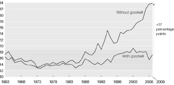
One of the main reasons for this phenomenon is how firms sustain abnormal growth rates. Firms growing often accumulate excess cash, which they use to make acquisitions. These acquisitions support growth and profitability, but acquiring firms must often pay a premium to convince target’ shareholders to sell. This premium over book value of the assets acquired generates goodwill. Operating returns exclude goodwill. The premiums paid, over book value, for acquisitions lower ROIC. Investors believe that goodwill will keep on reducing ROIC of all companies in the industry, thus attributing similar multiples to the peer group (see figure 4). The exceptions are usually companies which prove to investors their superior business model and superior capabilities.

FIGURE 4: ROIC, WITH AND WITHOUT ACCOUNTING FOR GOODWILL. SOURCE: THOMSON REUTERS

(27)

This thesis focuses on cash flow and relative valuation models. According to Damodaran (2002), the DCF approach is the basis of any valuation. Furthermore, Luehrman (1997) shows that APV is a useful tool and highlights information which are only implied in DCF approach. Lastly, Goedhart, Koller and Wessels (2005) refer the importance of using the multiples approach simultaneously with a cash flow based approach to improve its performance.

2.3. M&A-related topics

2.3.1. Return for shareholders

Mergers generally create economic value. Although the disparity of returns is high, depending on firm characteristics and the external environment, total shareholder return is, on average positive upon a merger (Bruner, 2005). Beyond whether M&A creates economic value, research has focused on the division of wealth created among acquirers and acquiring shareholders. Research points to the fact that the distribution of the gains in a merger is asymmetrical, skewed to favor acquired firm shareholders. Bruner (2005) concludes that shareholders of firms earn, on average, substantially larger returns than what was expected in an equitative distribution. The author also finds that, albeit shareholders within acquiring firms tend to profit little from acquisitions, they still manage to earn their return on investment rate. Acquiring firms hand-in most of the value created in a merger through the premium paid, thus retaining a relatively smaller share of value created.

Another way to look at this issue is by measuring market response, in the form of returns, to deal announcements. By studying the market performance of acquiring firms over a period of six years, Sirower and Sahni (2006) reach similar conclusions to Bruner (2005). Their research shows that acquirers had a return of -4.1% after the deal announcement. Furthermore, initial market response was found to be persistent over time. One year after the merger, acquirers maintained roughly the same return, at -4.3%. The opposite also holds: initially positive returns were still positive a year later.

In conclusion, there is strong evidence that M&A creates economic value and that it is asymmetrically distributed among target and bidder’s shareholders. Indeed, acquiring firms give away most of the synergies resulting from a merger to acquired shareholders, as the premium they pay to convince the target to the merger is often too high.

(28)

M&A transactions are typically of large size, comparing with the firm’s assets or revenues. Consequently, how a firm finances acquisitions has a large impact on the acquirers capital structure, namely ownership and financial leverage. The method of payment chosen, be it equity or debt, has severe impacts beyond capital structure, in areas such has taxation, corporate control and risk management.

From the above, it is understandable that managers and stakeholders face important decisions which can have deep consequences in firm value. The method of payment chosen for a deal is one such key decision. The choice between cash or stock as the deal currency is analyzed as a trade-off. If cash is used, leverage is required, which increases the cost of financial distress, diverts leverage capacity from other projects and can decreases managerial flexibility (e.g. through debt covenants). However, there is value created through tax shields and the acquirer is able to retain control over the merged entity. Although a stock deal is unlikely if the acquirer wants to preserve control, it is an attractive payment method if leverage capacity is either limited or available on relatively expensive terms, if the bidder’s shareholders do not assign much value to corporate control or if there is tax advantages (e.g. the ability to defer tax liabilities).

Faccio and Masulis (2004) performed an analysis on the trade-off between the use of cash and stock deals, weighing in corporate control against leverage limitations. The authors conclude that evidence suggests that the incentives to retain corporate control and use cash are strong when there are controlling shareholders of the bidder. Their analysis takes also into account market-to-book value of the bidders’ assets and share price behavior. These factors are found to be statistically significant explanatory variables for the chosen payment method.

2.2.3. Synergies

When two companies merge their combined value is usually greater than if those two firms operate independently. The additional value generated is synergies. These can take the form of operational synergies – such as economies of scale, greater pricing power and new growth potential – or financial synergies – such as tax benefits, efficient use of excess cash and diversification gains. Diversification as a source of financial synergy is possible although many argue that investors can diversify more efficiently on their own thus making this an inefficient and redundant move. Furthermore, the bidder often lacks the skills needed to run the target firm which can lead to worst performance of the acquired company. In turn, managers of the bidder can lose its focus thus affecting the performance of the acquirer, too. Doukas, Holmen

(29)

and Travlos (2001) find not only that investors are aware of these problems and react negatively to a deal with the intent of diversification but also that they are usually proven right, as the performance of the bidder deteriorates after the merger is completed.

Synergies create value either through an increase in cash flows or a decrease of the cost of capital of the combined entity. The value of the combined firm generally increases after the merger Bradley, Desai and Kim (1988). However, merging two firms can also destroy value, which is known as reverse synergies. In this case, the expected performance of the independent firms is adversely affected by the merger thus resulting less valuable merged entity.

Sound valuation of synergies is a critical success factor in any merger. This is rather complex because the acquirer can lack information about the target business and it relies on many assumptions regarding the future. It is also important to separate synergy value from value of control to avoid double counting.

Valuation should be done through a DCF analysis. The first step is to list all the expected synergies as well as the costs associated with them. Managers must assess synergies according to the costs required to secure them. Then, a timeframe must be developed to list those synergies in chronological order. While some synergies can be reaped almost immediately, others take longer. Failing to acknowledge this in the cash flow estimation leads to an inaccurate valuation which in turn can lead to a premium offered too high. Thirdly, both companies must be valued as independent entities. Finally, subtracting the value of the sum of both firms from the value of combined entity equals the value of synergies.

Additionally, accretive acquisition can be a motivation for engaging in an acquisition. Although its underlying assumption is that investors are irrational, the proposed value creation logic is that acquiring with lower earnings multiple than the acquirer will increase the multiple after the acquisition, matching the acquirer’s. That would translate into an immediate capital gain for the acquirer, once the merger was concluded.

2.2.3.1. SVAR

Synergies result from the performance improvements and value created when two firms are combined in a merger. Although synergies can express themselves in a number of forms, most commonly through increased revenues, cost reductions or lower cost of capital, ultimately, they are reflected in the present value of future cash-flows. These must be calculated before

(30)

deal is done and often without knowing the acquired firm in large detail. Besides the uncertainty of synergy materialization, evidence that acquirer’s pay too much for their acquisitions led to the need of developing a tool to measure how much acquiring firms’ shareholders stand to lose if the synergies proposed fail to materialize after integration. The SVAR is a tool to calculate synergy risk relative to shareholders’ wealth (i.e. market value of equity) (Sirower and Sahni, 2006). To compute SVAR, the premium paid is divided by the acquirer market value before the merger. The result is the percentage of shareholders’ equity at risk if synergies end up being null. In an all-stock deal, the formula is adjusted to incorporate the fact that the acquirer will only bear the synergy risk corresponding to its equity in the merged firm.

2.2.3.2. Operating Sense of Synergies

The success of a merger depends largely on the ability of the acquirer to increase the value of the merged companies so that the premium paid for the target’s shares is compensated by synergies and value of control. In other, words acquirers must meet the premium paid in the acquisition by cost or revenue synergies. So boards and managers should understand which cost decrease and/or revenue increase is required so that the premium paid is met, therefore making the merger worthwhile for the acquirers (Sirower and Sahni, 2006). The authors propose a method which resembles a breakeven analysis – by looking at the improvements in the bottom line sufficient to, at least, generate value equal to the premium paid. This analysis assumes that the already expected performance improvements as stand-alone businesses should not be included and must not be adversely affected by the merger, because this performance is already accounted for in the stock price, not the premium.

The method aims at informing about the required improvements which must take place with a simple formula which relates the premium offered, EBIT and cost and revenue synergies.

Where,

%SynC is the required percentage cost decrease to justify the premium

is the pretax profit margin

(31)

%SynR is the required revenue increase to justify the premium

This formula yields a range of possible combinations of cost and/or revenue synergies which compose the MTP (meet the premium) line. If the expected synergies fall below the line, then the merger will destroy value for the acquirer, at the premium currently offered. In turn, the expected synergy mix should always be above the line. To expand on this analysis, the authors question the cost base which can realistically be changed as well as the potential revenue improvements – which are usually much harder to anticipate and materialize in the short term. To address this question, the authors recommend looking at similar deals and at the cost structure of the business in order to generate a maximum plausible synergy mix, which values beyond are unrealistic. The premium offered must then be justified by improvements within the plausible range of synergy mix, or the Plausibility Box – values beyond the plausibility box can be the result of too optimistic assumptions.

FIGURE 4: MEET THE PREMIUM LINE . SOURCE: (SIROWER AND SAHNI, 2006)

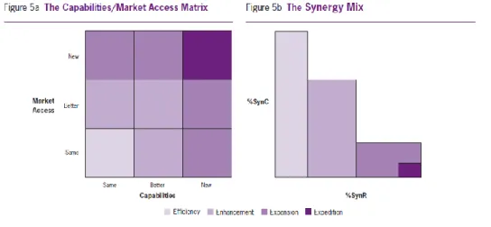
Sirower and Sahni (2006) consider a third question – is the combination of cost and revenue synergies proposed in the MTP method achievable in operating terms? The authors suggest a follow up of the proposed synergies which fall within the plausibility box based on the strategic nature of the deal and the type of assets and capabilities being brought together.

To answer the question, they developed a matrix relating the type of market access and capabilities of both parties. The matrix’s intent is to assess whether the synergies are viable given two parameters being evaluated, market access and capabilities. If the merging companies compete in different markets, then the merger will result in access to new markets for both firms. Conversely, if those companies are competitors, they can either improve their market access or it can remain unchanged. A similar analysis is performed on the capabilities

(32)

side. A merger can result in new capabilities for one or both firms but it can also improve or maintain them.

FIGURE 5: CAPABILITIES/MARKET ACCESS FRAMEWORK. SOURCE: (SIROWER AND SAHNI, 2006)

The characterization of the deal based on the matrix is followed by the categorization of the deal. There are four options:

1. Efficiency: The prospective merger brings together two similar companies in terms of market and capabilities. A deal of such kind should yield virtually no revenue synergies only elimination of redundant costs and scale economies (costs synergies).

2. Enhancement: Two companies with similar market access and capabilities can merge to form a company better positioned in competitive terms. These deals should form a cost and revenue mix, with scale economies combined with increased sales and new customers.

3. Expansion: When the overlap of capabilities and market access is limited but the companies improve their competitive positioning or expand into new segments, the deal results in mostly revenue synergies. However, cost synergies can still be reaped. 4. Expeditions: Deals between companies distinct from each other should have the

strategic rationale of increasing revenues, mainly through cross-selling. Expeditions happen when acquirers seek companies in different markets and fundamentally different business models than their own.

(33)

The authors propose this method to assess the potential synergies yielding from a deal. It should be used as a basis of discussion to the synergy mix, bearing in mind that if the synergy mix differs substantially from the category’s indicative synergy mix, its underlying assumptions must be reassessed.

3. Industry Review

3.1. Supply analysis

3.1.1. Introduction

The paper industry is capital intensive because the need to build production infrastructures, mainly paper and pulp mills, as well as distribution infrastructures, such as roads, railways and ports. The industry has been in decline in many of its segments, originating periods of excess capacity. Capacity available is quite constant over time because mills have a useful life of more than 30 years. However, the constant need to be efficient and innovative, driven by low margins across most segments, requires large investment in fixed assets periodically, when mills must be shut down and rebuilt to gain more efficiency.

3.1.2. Industry Mergers & Acquisitions

The industry relies on M&A to grow and achieve scale and scope. Organic growth is limited as opportunities are scarce in this mature and saturated industry. Firms in the western world are actively seeking higher exposure to fast growing emerging markets, experiencing stable or declining demand at home coupled with excess capacity. Consequently, the bulk of the investment in this industry is captured by emerging markets with comparative advantages vis-à-vis mature economies. The US-based International Paper acquisition of SCA’s Asian operations is an example of that.

Another industry trend, dating back almost a decade, is the consolidation of supply in Europe and the US, as firms look for scale to improve margins. The 2010 UPM acquisition of Finnish firm Myllykoski was completed with the main strategic rationale being improving profitability through building scale. M&A is also driven by deals intended to retire capacity of the market. There is persistent over capacity in mature markets across most segments, which drives down prices. To counter this, the major players are acquiring competitors and shutting down their older, inefficient mills. International Paper announced in the end of 2013 the shutdown of its largest paper mill, citing shrinking demand due to switch to online format and the need to take

(34)

capacity off the market. In China, similarly, tackling excess capacity has been conducted through a government program mandated to shut down inefficient paper and pulp mills.

3.1.3. Business Segments

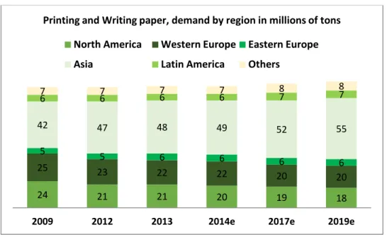
The global paper and pulp industry competes with other industries in the procurement of wood, its main raw material. There are a few different types of wood which are transformed into cellulose, the main component of most kinds of paper apart from recycled fibers. The industry’s output can be segmented into five groups of products: Printing and writing paper, newsprint paper (used in newspapers and magazines), tissue paper, container board (used in paper packages) and other types of paper and paperboard (paper bags, filters, etc). The scope of this thesis only concerns the printing and writing paper segment, the only type of paper produced by Portucel and the main type produced by Suzano. This segment has similar raw material (wood logs) but its transformation is quite distinct from other segments. The end users as well as the distribution channels are also different which makes this segment a rather independent business from the rest of the industry.

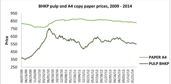
FIGURE 6: PULP AND PAPER INDEX PRICES. SOURCE: FOEX INDEXES

The industry is primarily composed of integrated paper producers. An integrated producer has industrial units with a pulp and paper mill connected. Once the raw material is transformed in the pulp mill, into pulp, it directly enters the paper mill. This means that paper mills which source pulp from elsewhere are an exception. This organization of production is optimal because pulp prices are volatile while paper prices tend to be constant over time (see Figure 6). The industry’s inability to pass higher input (i.e. pulp) costs to customers has led to the need to hedge against pulp price volatility or otherwise face unpredictable and highly volatile

250 350 450 550 650 750 850 950 04/ 07/0 9 06/ 16/0 9 08/ 25/0 9 11/ 03/0 9 01/ 12/1 0 03/ 23/1 0 06/ 01/1 0 08/ 10/1 0 10/ 19/1 0 12/ 28/1 0 03/ 08/1 1 05/ 17/1 1 07/ 26/1 1 10/ 04/1 1 12/ 13/1 1 02/ 21/1 2 05/ 01/1 2 07/ 10/1 2 09/ 18/1 2 11/ 27/1 2 02/ 05/1 3 04/ 16/1 3 06/ 25/1 3 09/ 03/1 3 11/ 12/1 3 01/ 21/1 4 Pr ic e

BHKP pulp and A4 copy paper prices, 2009 - 2014

PAPER A4 PULP BHKP

(35)

costs and, consequently, unpredictable margins. This has led to many firms experiencing financial problems in the past as firms are usually highly geared in this industry.

Firms could simply hedge input price volatility recurring to contracts or financial derivatives. However, firms chose to hedge through producing and stocking a part or the whole of their pulp needs. The chosen hedging mechanism has to do with costs associated with sourcing pulp externally which are not occurred in the integrated production system. Pulp has a high percentage of water in its composition. To produce paper, pulp must retain a high degree of water composition. However, transportation of wet pulp is too expensive due to its weight, substantially higher than the weight of dried pulp. As a consequence, to reduce transportation costs, pulp is dried before shipping. When it reaches its final destination, the paper mill, the dried pulp has to be splashed with water to regain the desired humidity. The cost of doing this is eliminated in the integrated production system which confers a cost advantage to integrated firms.

There is still a global market for pulp. The main players are firms which have excess/deficit of pulp as paper production input for their own mills and paper firms which are not integrated, around 15% of total firms.

3.1.4. Industry Consolidation

FIGURE 7: NUMBER OF MILLS AND TOTAL PULP PRODUCTION VOLUME IN EUROPE. SOURCE: CEPSI

The industry has been going through a trend, since the beginning of the XXI century, towards supply consolidation. Although it is an industry wide trend, it has been experienced in larger degree in the mature markets of North America and Western Europe. Indeed, either through M&A activity or bankruptcy, the number of mills has been decreasing while production has