Comparative study of NETmix and T-jets reactors based on pressure dynamics

(1)

Comparative Study of NETmix® and T-jets Reactors

Based on Pressure Dynamics

Master Thesis

by

Mumin Enis Leblebici

Developed within the discipline of Dissertation at

LSRE – Laboratory of Separation and Reaction Engineering

Supervisors: Prof. José Carlos Lopes

Doutor Ricardo Jorge Nogueira Santos

Departamento de Engenharia Química

(2)

i

Keep on learning and thinking…

Learn at the expense of:

Laziness and pleasure

Bliss of Ignorance

Living easier

Dr. Feridun Bilginer

(My Grandfather)

(3)

ii

ACKNOWLEDGEMENTS

I would like to express my gratitude and respect to my supervisors Prof. José Carlos Lopes, and Dr. Ricardo Santos who gave me a chance to be in their team and made this work possible by their guidance, help and patience.

I would like to express my gratitude to Prof. Madalena Dias for her patience, time and effort. I would like to thank Prof. José Miguel Loureiro for his support and advice along the way.

I would like to express my special thanks to my colleagues and friends Carlos Fonte and Cláudio Fonte who taught me a lot and walked with me along the path to finish this work.

I would like to thank my friend Telmo Santos who made possible the data acquisition part of this work. Without his technical support as well as company and friendship, life in the laboratory would be much harder without a doubt.

I would like to thank Mohamed Ashar Sultan for his help and support during T-jets experimental phase of the work.

I would like to thank Anna Karpinska Portela, Ângela Novais, Marina V. Torres, Kateryna Krupa for their friendship as well as technical support along the way. I am proud to be in a team with these people.

I would like to thank my dear friend Paulo Gomes for all his help and support along the way. I would like to express my special thanks to my dear friend Erdem Demir who was with me from the beginning to the end with his smiling face and bright mind. I don’t think I will ever eat such delicious chicken wings again.

I would also like to thank my dear friends Filipe Madureira and Nuno Gonçalves for being such good friends and supporting me along the way.

I would like to thank my mother and father who trusted me and supported me through this way. Their love, patience and support have always been invaluable for me.

I would like to thank Allan Martin Edwards not only for making this step of my life possible but also trusting me and making me feel I have another family member I can trust and talk to. Last but not the least, I would like to thank my girlfriend Pelin Arslan, for her huge heart, endless love, patience and tranquillity which gave me power till the end.

(4)

iii

ABSTRACT

Static mixers are newer designs of mixers compared to agitated tanks. They use the energy supplied by the inlet flow stream in order to induce mixing. Various designs are available in the global market since 1960s. This work focuses on two static mixer designs. The first, NETmix®, is a patented invention from research at LSRE – FEUP. The other design is T-jets geometry, which is commonly used in reactive polymer processing or nanoparticles production.

Main goal of this work is to measure correctly the pressure drop along NETmix® and T-jets mixers and to develop a model that describes it. Comparison of these two mixing technologies will also comprise the computation of the actual the energy used on mixing. Furthermore, computational fluid dynamics (CFD) simulations and visualization of the flow characteristics, are used to gain insight into the mechanisms that influence the pressure drop of different designs of the mixers.

To obtain pressure drop values, differential pressure sensors were coupled to the inlets and outlets of various NETmix® and T-jets mixer prototypes. After obtaining the pressure drop data for different geometries and fluids properties, a previously introduced network model was fitted to the results with one adjustable variable.

Power number and Z factor were used to compare the energy efficiency and pressure drop

performance of NETmix® and T-jets mixers as well as popular static mixers today in the market. Furthermore, dynamic pressure measurement were made in the NETmix® reactor to assess the flow dynamics and a model for it was proposed and validated from experimental data.

(5)

iv

RESUMO

Os misturadores estáticos são uma nova tecnologia em relação aos mais tradicionais tanques agitados. Estes misturadores utilizam a energia das correntes de alimentação ao reator para promoverem a mistura. Este trabalho foca-se em dois misturadores estáticos. O primeiro é o NETmix®, uma tecnologia introduzida e patenteada no LSRE – FEUP. A outra tecnologia são os misturadores de jatos em T, e são utlizados no processamento reativo de polímeros e na produção de nanopartículas.

O principal objetivo deste trabalho é a medição da queda de pressão no NETmix® e em misturadores de jatos em T, e a introdução de um modelo que descreva a queda de pressão. Este estudo vai ainda abordar a comparação da energia despendida na mistura nas duas tecnologias. Os mecanismos responsáveis por diferentes desempenhos de diferentes geometrias dos misturadores são analisados a partir de simulações de computação de fluidos dinâmicos (CFD) e de experiências de visualização.

As quedas de pressão foram obtidas com transdutores de pressão diferenciais ligados às entradas e saídas de diferentes geometrias de misturadores NETmix® e de jatos em T. Obtida a queda de pressão para diferentes geometrias e propriedades de fluidos, um modelo de redes, com uma variável ajustável, foi aplicado aos diferentes misturadores.

O número de potência e o fator Z_{foram usados para comparar o desempenho de diferentes}

geometrias do NETmix® e de misturadores de jatos em T. Estes misturadores foram também comparados com misturadores estáticos comerciais sobre os quais havia dados disponíveis.

A medição dinâmica da pressão foi utilizada para avaliar a dinâmica de mistura em reatores NETmix®. A partir dos dados experimentais propôs-se um modelo para a dinâmica dos escoamento no misturador NETmix®.

(6)

v

INDEX

LIST OF FIGURES ... vii

LIST OF TABLES...x

1 INTRODUCTION ... 1

1.1 Motivation and Relevance ... 1

1.2 Thesis Objective and Layout ... 3

2_{STATE OF THE ART ... 4}

2.1 Static Mixers ... 4

2.2 Hydrodynamics and Benchmarking Static Mixers ... 5

2.2.1 Pressure Drop Benchmarking ... 5

2.2.2 Energy Dissipation Benchmarking ... 7

2.3 Description and Comparison of Some Conventional Static Mixers ... 8

2.3.1 KM®_{Kenics Static Mixer – Chemineer INC ... 8}

2.3.2 SMX® and SMV® – Sulzer Chemtech INC ... 9

2.3.3 Inliner - Lightnin INC ... 10

2.3.4 ISG Mixer – Ross INC ... 10

3_{NETmix® Static Mixer ... 11}

3.1 NETmix® Concept and Description ... 11

3.2 NETmix® Experimental Set-Up ... 12

3.3 NETmix® Pressure Drop ... 15

3.3.1 Pressure Drop Model ... 15

3.3.2 Pressure Drop Results ... 18

3.4 Frequency of Oscillation for NETmix® ... 20

(7)

vi

4.1 T-jets Concept and Description ... 24

4.2 T-jets Experimental Set-Up ... 25

4.3 T-jets Pressure Drop ... 28

4.3.1 T-jets Pressure Drop Model ... 28

4.3.2 T-jets Pressure Drop Result ... 29

4.4 Tracer experiments ... 31

4.5 T-jets Energy Dissipation ... 33

4.6 T-jets CFD Simulations ... 34

4.6.1 CFD Model ... 34

4.6.2 Effect of Depth in T-jets Geometry ... 35

4.6.3 Effect of Channel Width in T- Jet Geometry ... 36

5_{Assessment of Different Static Mixers ... 37}

5.1 Power Number Comparison ... 37

5.2 Z factor comparison ... 38

6_{CONCLUSIONS ... 41}

7 EVALUATION OF THE WORK ... 43

7.1 Accomplished Goals ... 43

7.2 Limitations & Future Studies ... 43

REFERENCES ... a APPENDIX – 1 ... c APPENDIX – 2 ... e APPENDIX – 3 ... f APPENDIX – 4 ...g APPENDIX – 5 ... i APPENDIX – 6 ... j

(8)

vii

LIST OF FIGURES

Figure 1 An aluminium T-jets mixer ... 2

Figure 2 Tracer experiment in a NETmix® prototype [7]. ... 2

Figure 3 KM® Static mixer [12]. ... 8

Figure 4 a) SMX®; b) SMV® static mixers pipe inserts [14] ... 9

Figure 5 Inliner series static mixing insert [15] ... 10

Figure 6 a) ISG pipeline inserts; b) horizontal cut of 5 mixing chambers of ISG mixer[16] ... 10

Figure 7 (a) NETmix® geometry, (b) CSTR and PFR model analogy[4]. ... 11

Figure 8 Unit Cell for: a) NETmix® 3D and b) NETMix® 2D [17]... 11

Figure 9 NETmix® prototypes: a) NETMix® 3D; b) Multi-Inlet NETmix® 2D; c) Lab-scale NETmix® 2D. ... 12

Figure 10 General scheme of NETmix® pressure drop measurement setup. ... 13

Figure 11 NETmix® 2D setup: 1-support structure, 2-NETmix reactor, 3-peristaltic pump, 4-pressure transducer, 5-indicator, 6-oscilloscope. ... 14

Figure 12. LabView user interface for NETmix®. 1-data record file name, 2-data acquisition rate, 3-unfiltered and filtered signal graph, 4-FFT processed but unfiltered signal, 5-FFT processed filtered signal, 6-oscillation filter band selection. ... 14

Figure 13 Oscillation measurements set-up: a) drilled channels; b) system connected to the experimental setup. ... 15

Figure 14 Pressure drop model with resistance in the channels ... 16

Figure 23 T-jets geometries: (a) photograph (b) schematical view. ... 25

Figure 24 T-jets mixer mounted on acrylic block. ... 26

Figure 25 General scheme of T-jets experimental set-up. ... 26

Figure 26 T-jets experimental setup: 1-T-jets, 2-pressure transducer, 3-control valves,

4-pressurized vessels, 5-camera, 6-computer. ... 27

Figure 27 T-jets LabView interface: 1-input knob, 2-automatic input values, 3-data series record domain, 4-pressure drop value, 5-fluid and geometry parameters, 6- measured flowrate, 7- data acquisition rate, 8- raw signal and FFT graph. ... 27

Figure 28 T-jets scheme showing the calculation of

L

*_{. ... 29}

Figure 29 Plot of pressure drop versus Reynolds number for different T-jets depth values; lines represent the pressure drop model fitted for each geometry. ... 30

Figure 30 Plot of pressure drop versus Reynolds number for different T-jets channel width values; lines represent the pressure drop model fitted for each geometry... 30

Figure 31 Effect of depth (a) and channel width (b) on the fitted values of

K

. ... 31

Figure 32 T-jets tracer experiments for W6w1d1 geometry at

Figure 41 Z factor versus Reynolds number for the NETmix and T-jets geometries in comparison with conventional static mixers. ... 40 Figure 42 Calibration curve for diaphragm number 30 ... d Figure 43 Calibration curve for diaphragm number 36 ... d

(11)

x

LIST OF TABLES

Table 1. Comparison of the static mixers with conventional agitated tank mixer. ... 4

Table 2. NETmix®_{prototypes ... 13}

Table 3 List of studied T-jets reactors geometrical parameters. ... 25

Table 4 Fitted

K

values for the studied T-jets geometries. ... 31

(12)

1

1 INTRODUCTION

1.1 Motivation and Relevance

The word “reactor” would probably flash a picture of a mixing tank in a chemical engineer’s mind. This fact is quite normal since chemical reactors, being the heart of chemical production in many industrial applications, are machinery, designed based on mixing principles with the majority of them being simply mixers of different scales. An efficient mixing is generally desired in the reaction step of chemical production[1]. Reactors control the contact performance of different chemical species for mass transfer while supplying required physical conditions (e.g. temperature, pressure) in order to get the highest possible yield out of the reactants. They input the required energy to increase contact area and thus, mass transfer rate between species. However, the idea of mixing started to deviate from simple shaft driven tank mixers when the first static mixers were developed for the fiber industry [2]. Along the way, this new technology evolved to fit a wide variety of different scales and applications while this work will be focusing on lower scale applications, namely micromixers, specifically on opposed jet mixers, investigating them from the hydrodynamics point of view.

Opposed jets mixers are mainly used for mixing under fast chemical reaction processes, where the limiting step is the reactants’ contact time[3]. This work focuses on T-jets and NETmix®

geometries as opposed jet applications. A pressure drop model was put to test for the NETmix®

mixer, while the hydrodynamics such as mechanical energy dissipation, power number and

Z

factor were investigated to assess the performance of the systems as well as for the comparison with conventional mixers.

T-jets consists on the impingement of two liquid streams of reactants in a confined chamber (Figure 1). The most commonly used industrial application of these devices is in reaction injection molding (RIM) which usually consists of cylindrical jets and chambers with extremely low residence time, less than a tenth of a second. High velocity jets and low residence times give a uniformly mixed output that is ready to be molded as the reaction actually takes place within the mold. This way, high volume molding applications of fast-curing polymers just like polyurethane are performed. The T-jets geometries studied in this work are different from existing industrial versions, consisting of rectangular prism channels and chamber.

(13)

2 Figure 1 An aluminium T-jets mixer

NETmix® is a new concept of static mixing consisting of a network of interconnected channels and chambers within a two dimensional geometry [4], developed and patented[5] at Faculty of Engineering University of Porto, Laboratory of Separation and Reaction Engineering (LSRE). The NETmix® model is the basis of a flow simulator coupled with chemical reaction used to characterize macro and micromixing in structured porous media [4]. NETmix® was applied for the production of nanocrystalline hydroxyapatite [6] with controlled particle size distribution [5]. Figure 2 shows a tracer experiment in a NETmix® prototype.

(14)

3

1.2 Thesis Objective and Layout

Past technological developments and recent novel studies on static mixing will be summarized in the Chapter 2. Comparison tools will be given as well as some popular conventional designs which have been used till today will be introduced.

NETmix®_{concept description, the used experimental setups and model will be introduced in}

Chapter 3. Results obtained from NETmix®_{will also be given in this part of the work.}

Chapter 4 describes the T-jets concept as well as the experimental prototypes used for this work. This chapter will also include Computational Fluid Dynamics (CFD) and experimental results on this static mixer.

In Chapter 5, assessment of the considered mixers will be performed comparing also with the conventional designs.

Chapter 6 is dedicated to the conclusions of this work.

Finally, in Chapter 7, an overall evaluation of the project will be presented and future work will be suggested.

(15)

4

2 STATE OF THE ART

2.1 Static Mixers

Mixing, although being one of the most fundamental unit operations in chemical engineering science, was almost left alone, until the development of the first connection to reaction engineering by Danckwerts in early 50’s. Before this, the study of mixing methods were suffering from the lack of any quantitative methods to assess “the goodness of mixing”[8]. Furthermore, mixing devices were very close to the ones used in 16th_{century as described by Ottino [9].}

However, not all the mixing needs of the industry were of the same nature. There were fast reactions achieving equilibrium within microseconds as well as slower ones, which needed hours. There also were viscous materials to be mixed which needed very high power input as well as low viscosity applications. All those different needs meant different machinery, however the options in the inventory were very limited when it came to viscous fluids and/or fast chemical reactions.

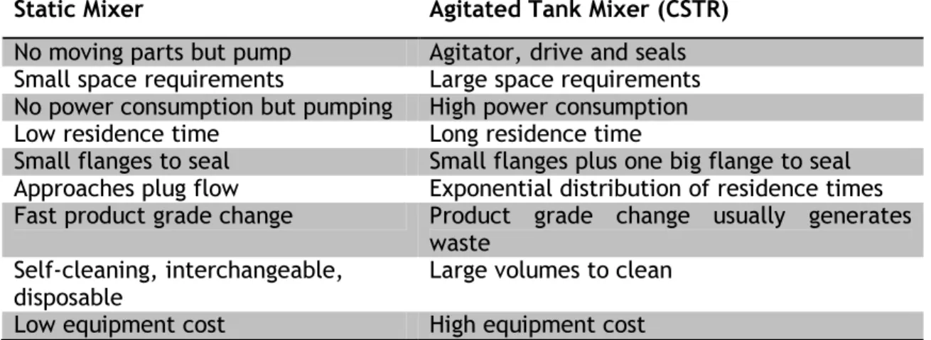
Static mixers were developed first in order to overcome the difficulties in the mixing operation of high viscosity polymer components of synthetic fiber industry [2, 10]. This invention was revolutionary in related industries since homogenization of the high viscosity fluids with conventional mixing devices meant much higher operation costs as well as maintenance cost than these new mixing devices [11]. Other potential advantages of static mixing units are listed in Table 1.

Table 1. Comparison of the static mixers with conventional agitated tank mixer.

Static Mixer Agitated Tank Mixer (CSTR)

No moving parts but pump Agitator, drive and seals

Small space requirements Large space requirements

No power consumption but pumping High power consumption

Low residence time Long residence time

Small flanges to seal Small flanges plus one big flange to seal

Approaches plug flow Exponential distribution of residence times

Fast product grade change Product grade change usually generates

waste Self-cleaning, interchangeable,

disposable Large volumes to clean

Low equipment cost High equipment cost

Despite the revolutionary advantages of this new technology, in the early 1970’s, when it became a process standard for polymer homogenization, the design was yet, far from being

(16)

5 perfect. Charles Potter, inventor of the first Kenics Static Mixer, claims that these units had to be flushed with solvent once in a few hours and also needed replacement with a new or clean one, every two weeks [10].

As in all the commercial products, market demand and different application possibilities resulted in competition and different designs. In the following sections, the most popular designs will be compared, summarizing hydrodynamic properties, and the applications that they are usually utilized and working principles.

2.2 Hydrodynamics and Benchmarking Static Mixers

An analogy with automotive industry can explain the relationship between hydrodynamics and mixers. There are designs for heavy-duty transportation and designs for light and fragile sports car, both bearing cutting edge technology. The distinction between those designs would be parameters such as speed, engine power, durability, volume of transport. Values of all the parameters stated, would characterize the design to be a “truck”, a “bus”, a “passenger car”, or a “sports car”. In mixers the parameters would be mixing time, total holdup volume, pressure loss, and quality of mixing. All the devices and machinery as well as the application itself coupled to the mixer, should be chosen considering the hydrodynamics of the mixer.

The following sections will summarize the benchmarks that were focused in this work to decide if the considered designs are “trucks” (mixing large amounts of materials slowly but with a low pressure drop) or “sports vehicles” (achieving complete mixing very fast compromising the pumping cost due to high pressure drop).

2.2.1 Pressure Drop Benchmarking

The main parameter to be observed in order to compare the pressure drop performance of the commercial designs with both NETmix®_{and T-jets mixer reactors will be the}

Z factor [11], defined as mixer emptypipe

P

Z

P

∆

=

∆

(1)

where

∆

P

_mixer is the pressure drop along the mixer, while ∆P_emptypipe is the pressure drop resulting

only if the fluid was flowing in an empty pipe with an equivalent diameter and length. The Z

factor is essential for any mixer for the calculation of the pumping costs as well as comparing different designs. No matter what the application the mixers are used for, or the scale of the material flowing through, the Z factor normalizes the energy consumed on pumping.

(17)

6 In other words, mixer A coupled to system X may cause a pressure drop of 5000 Pa while mixing 2 m3_{of material through 2 m of 3 inch equivalent pipe. Whereas, mixer B coupled to system Y}

may cause a pressure drop of 5 Pa while mixing 0.01 m3_{of material with different viscosity and}

density through 0.3 m of 1/2 inch equivalent pipe. Their benchmarking from the energy efficiency point of view can only be established by normalizing the work done on the flowing fluid, to a dimensionless quantity, which in this case will be Z.

To be able to achieve the Z value for each design, pressure drop values have to be correctly

obtained. Equation 2 will be used to yield these values [11] concerning the flow to be in laminar regime. 2

2

e e

f

P

NL

d

ρν

∆ =

(2)

where,

f

is the friction factor,

ρ

is the liquid density,

ν

is the fluid velocity through the equivalent pipe,

d

_e is the equivalent pipe diameter,

N

is the number of mixing units and

L

_e is equivalent length of each mixing unit.

In general the friction factor is obtained by

16 Re

ρ

ude

µ

= (4)

where

µ

is the fluid viscosity. For an empty tube

f

_{is given by Fanning’s equation}

16 Re

Fanning

(6)

(18)

7 The equivalent pipe geometry is straightforward for conventional static mixer units, as they are just pipes with different packings. However, for the NETmix®_{and T-jets geometries, an}

equivalent pipe geometry is defined by Laranjeira [7] and will be explained in detail in the corresponding sections.

2.2.2 Energy Dissipation Benchmarking

The time passing from the first contact of the reactants until the perfectly homogeneous mixture may sometimes define the path the reaction mechanism follows and therefore is very important. This mixing time, in the case of rapid reaction kinetics, needs to be as short as milliseconds. Since fluid mixing is the increase of interfacial area between species and the energy needed to increase this contact area is provided by the mixing medium, this energy divided by the mixing time yields the power input to the fluid. This desired mixing action can be assessed by determination of the rate of the real work done on the fluid, by the mixing device. Thus the second parameter to be considered for comparison of different systems is the energy dissipation defined by

_p, used to assess mixing in stirred tanks [12], defined as the ratio between the total amount of power supplied to the tank and the power used only for mixing and it may be defined in terms of the corresponding pressure drop terms

mixer P mixer friction

P

N

P

∆

=

∆

− ∆

(8)

(19)

8 where

∆

P

_mixer is the total pressure drop in the mixer and

∆

P

_friction is the pressure drop due to friction only. For both T-jets and NETmix®, the power number will be used to assess the energy transfer to the fluid whereas compound energy dissipation will be used as well but only for the T-jets mixer. However for the rest of the commercial designs due to the lack of data in the literature, energy efficiency benchmark will not be used.

2.3 Description and Comparison of Some Conventional Static Mixers

2.3.1 KM®

Kenics Static Mixer – Chemineer INC

Being the first static mixer design and due to its popularity in North American industry, Kenics is the most studied among the static mixers. Helical inserts within pipelines are oriented to rotate the flow to opposite directions at every mixing unit. This action causes chaos and thus, mixing by stretching and folding. A representative image of this design is shown in Figure 3.

Figure 3 KM® Static mixer [12].

This static mixer is used for laminar (mainly polymers and high viscosity materials) and turbulent (low viscosity) mixing in gas, liquid/liquid, and liquid dispersions systems.

Friction factor data was studied in detail by Cybulski et al. [13] and reported by Thakur et al. [11]

85.3

0.34 Re

P

f

_∆

=

+

(9)

However, since this mixer is a slow mixer and not used for fast reactions energy dissipation data is not available in the open literature. Competitiveness of this design originates from its low pressure drop.

(20)

9

2.3.2 SMX® and SMV® – Sulzer Chemtech INC

These two different geometries are designed by the same company but for two separate static mixing applications and markets.

• SMX® pipeline insert static mixers (Figure 4a) are lower pressure drop and slower mixers for tough mixing jobs such as dispersing a low viscosity fluid in a high viscosity medium[14]. It is also used for gas-liquid contact. Equation 10 summarizes the pressure drop behaviour of this mixer with respect to Re.

160

960 to

Re

P

f

_∆

=

(10)

• SMV® inserts (Figure 4b) have a similar design, however the higher pressure drop is compromised an mixing is speed up. This geometry is more frequently used in turbulent flows and gas-liquid contact. Sulzer INC. mentions “fast and complete reaction, absorption or extraction due to high mass transfer area” as the product description [14].

Cybulski et al. [13] have also calculated the energy dissipation figures for this geometry so that the Z factor can be obtained.

(a) (b)

Figure 4 a) SMX®; b) SMV® static mixers pipe inserts [14] Friction factor and the energy dissipation relations forSMV® mixers are given by

1040

4800

Re

P

f

_∆

=

to

(11) 2

793 /

262 /

W kg

turbulent regime

W kg

ε

′ =

=

(12)

(21)

10 2.3.3 Inliner - Lightnin INC

Another competitor of mixing market is Lightnin INC. This company released only one series of static mixers to date, referred as the Inliner static mixer (Figure 5).

Figure 5 Inliner series static mixing insert [15]

This mixer’s pressure drop factor has been reported previously [13] and given as

144 Re

P

f

_∆

=

(13)

2.3.4 ISG Mixer – Ross INC

Interfacial Surface Generator static mixer from Ross INC has a special meaning for this work since this geometry shares some fundamental principles with NETmix® geometry as ISG unites and divides the flow as seen in Figure 6 [16]. Being a high pressure drop design, it is used for the mixing of materials with viscosity ratio up to 250 000/1 [16].

(a) (b)

Figure 6 a) ISG pipeline inserts; b) horizontal cut of 5 mixing chambers of ISG mixer[16] The pressure drop factor of this mixer has been investigated by Cybulski and Werner [13] and given by

4000

4800

to

Re

P

f

_∆

=

(14)

(22)

11

3 NETmix® Static Mixer

3.1 NETmix® Concept and Description

NETmix® is a new type of static mixer [4, 17] that consists of a 2D network of chambers interconnected by channels as represented in Figure 7a. The network is constructed by the repetition of a unit cell, shown in Figure 8, where each chamber has two inlet and two outlet channels placed at a 45º angle. The network size is given by the number of rows,

n

_x, and number of columns,

n

_y which also defines the number of inlets. The direction of the flow is assumed to follow the

x

-axis.

Figure 7 (a) NETmix® geometry, (b) CSTR and PFR model analogy[4].

(a) (b)

Figure 8 Unit Cell for: a) NETmix® 3D and b) NETMix® 2D [17].

The unit cell can have two geometries. The first geometry (Figure 8a) has spherical chambers characterized by the diameter D and cylindrical channels with diameter

d

and it is refereed as the NETmix® 3D [29]. In the second geometry (Figure 8b) the chambers are cylinders with diameter D and thickness

ω

and the channels have rectangular cross section prims with width

(23)

12 Mixing in NETmix® can be controlled effectively making it particularly suited for complex and fast kinetics reactions. A NETmix® model has been developed [4] with the chambers modelled as complete mixing zones (Continuous Stirred Tank Reactor, CSTR) while the channels are complete segregation (Plug Flow Reactor, PFR) units as seen in Figure 7b. Mixing occurs along the structure, in the chambers by the aid of the impingement of the jets that are formed by the inlet channels [7]. It has been shown the existence of a critical Reynolds number for the onset of mixing that occurs when the two inlet jets impinge in the chamber and start to oscillate, this results in the chamber to act as a complete mixing zone that divide the flow by the two outlet channels that will form new jets and feed the next two downstream chambers [17].

3.2 NETmix® Experimental Set-Up

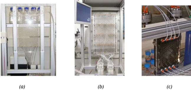
Three NETmix® prototypes, shown in Figure 9 were used for the experiments conducted in this work. The geometry and dimensions of each prototype are given in the Table 2. The first is a NETmix® 3D geometry (Figure 9a)][4, 17] and the other two are NETmix® 2D geometries. One is a large scale prototype with multi inlets rows, called the Multi-Inlet NETmix® 2D [18]. The third is a small, laboratory scale test unit.

(a) (b) (c)

Figure 9 NETmix® prototypes: a) NETMix® 3D; b) Multi-Inlet NETmix® 2D; c) Lab-scale NETmix® 2D.

(24)

13 Table 2. NETmix®_prototypes

Geometry NETmix® 3D Lab-scale NETmix® 2D Multi-Inlet NETmix® 2D Number of rows,

n

_x 49 29 65 Number of columns,

n

_y 15 8 16 Chamber diameter,

D

(mm) 7 6.5 8.75 Channel diameter/width,

d

(mm) 1.5 1 1.5 Geometry depth, ω (mm) ― 3 5.9 Channel length,

l

(mm) 3 2 5.4 Total volume (ml) 140 23 1500

A general scheme and a photograph of the experimental set-up for pressure drop measurements are shown in Figures 10 and 11. Water and 10%, 20% and 60% glycerol aqueous solutions were used to validate the pressure drop model in laminar flow regime. n-Octene was used to assess the pressure drop behaviour of the Lab-scale NETMix® 2D mixer in turbulent regime. The pressure sensor and indicator were calibrated for every set of experiments. The differential pressure transducer was equipped with membranes of 36, 26 and 22 calibre for different pressure drop ranges. The pressure indicator sends voltage data to the oscilloscope and/or to the computer via a data acquisition board from National Instruments.

For the pressure drop vs.

Re

results, four voltage values were read from the indicator to interpret how the pressure drops along the mixer by the aid of the calibration curve obtained and for each flow rate four measurements were made with a 500ml graduated cylinder at the outlet and a 1/100s stopwatch.

For the oscillation frequency measurements, data was recorded and processed by a LabView interface. An oscilloscope was also utilized as standalone for data recording. Instructions on calibration and operation of this system are given in detail in the Appendix 1.

Figure 10 General scheme of NETmix® pressure drop measurement setup. NETmix®

(25)

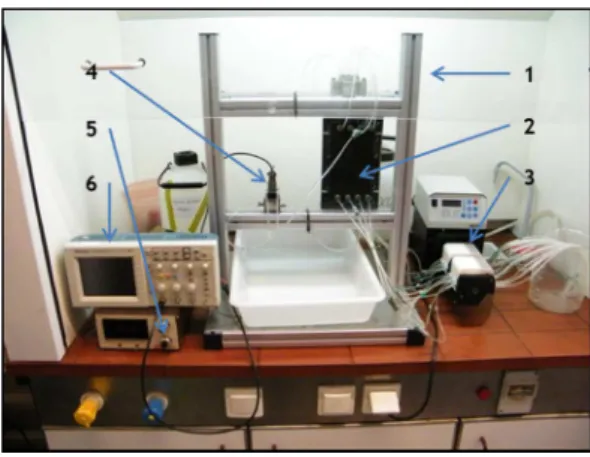
14 Figure 11 NETmix® 2D setup: 1-support structure, 2-NETmix reactor, 3-peristaltic pump,

4-pressure transducer, 5-indicator, 6-oscilloscope.

The data acquired from the transducer indicator is in Volts and is recorded at 500Hz by on-board DAQ card of National Instruments. This time series is then processed by a LabView application and also recorded to the user defined domain as shown in Figure 12 which works on the block diagram which is shown in Appendix 2. Voltage data obtained was converted to pressure units by the aid of the calibration line of the transducer to calculate the pressure drop along NETmix®. Monitoring the oscillation data was performed by changing the pressure transducer inlets to the outlet channel holes and recording the pressure data along the time series. The recorded time series (voltage vs. time data) is then filtered by a band-pass filter to eliminate 0-2Hz and higher than 40Hz oscillations since this range, can only occur due to the noise in the system. However, apart from this filtered range, any oscillation presence would indicate or a pump-induced oscillation, which is easy to predict, or self-sustained oscillation of the NETmix® as explained in section 3.4.

Figure 12. LabView user interface for NETmix®. 1-data record file name, 2-data acquisition rate, 3-unfiltered and filtered signal graph, 4-FFT processed but unfiltered signal, 5-FFT

(26)

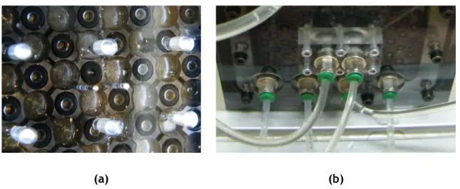
15 In order to measure the oscillation in a chamber the top cover was drilled to monitor the pressure of two outlet channels from the same chamber (Figure 13a,) that are then connected to the pressure transducers (Figure 13b). Keeping the same setup as pressure loss measurement but only changing the pressure transducer’s inlet position to the chamber outlets, the oscillation could be monitored.

(a) (b)

Figure 13 Oscillation measurements set-up: a) drilled channels; b) system connected to the experimental setup.

3.3 NETmix® Pressure Drop

3.3.1 Pressure Drop Model

The flow hydrodynamics in NETmix® has been modelled using an analogy with an equivalent resistance circuit as shown in Figure 14 [7]. The pressure drop in each circuit branch is given by

channel

P

R q

∆ =

(15)

where R is the branch hydraulic resistance and

q

is the flow rate through the respective channel.

The first pressure drop estimations in NETmix® were done considering a linear model with only friction effects in the channels [7], where

2 1 2 F channel h q l R R f d A

ρ

= = (16)

where RF is the friction resistance,

f

is the friction factor, l is channel length,

d

_h is channel hydraulic diameter, and A is channel cross-section area. For laminar flow

(27)

16

64 Re

f

=

(17)

where the Reynolds number is defined using the channel hydraulic diameter and the channel mean velocity,

v

=

q

_channel

/

A

, that is

Re

=

ρν

d

h

µ

(18)

Figure 14 Pressure drop model with resistance in the channels

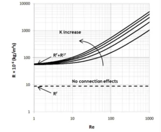
This model neglects the pressure loss due to the contractions and expansions that occur between channels and chambers. Here a complete model to predict the pressure drop developed by Martins et al. [19] is used. The total resistance is now given by the sum of the channel friction resistance, RF given by Equation 16 and two additional terms related to the contraction and expansion of the flow, a laminar, RLF, and a non-laminar, RNLF, flow resistances.

F LF NLF

R=R +R +R (19)

The laminar flow resistance term was defined by Koplik [20]

* 2 1 2 LF channel h q L R f d A

ρ

= (20)

This resistance exists wherever an unbounded jet flow is to be considered. When the fluid leaves the channel, the canonical friction term cannot model the energy transfer in the chamber as the flow is not bounded by the channel walls. Instead, the fluid’s solid channel is replaced with a viscous surrounding and as long as the jet keeps its form, the pressure drop can be modelled by this linear flow resistance term. According to Koplik

*

2d

L

π

(28)

17 is the distance the impinging jet maintains its form within the chamber.

The nonlinear contribution of contraction/expansion resistances at the inlets and outlets of a chamber can be expressed as

2 1 2 NLF qchannel R K A

ρ

= (22)

where K is a coefficient analogous to the coefficients for sudden contractions and expansion, generally used in the calculation of pressure losses in pipe systems. K is an adjustable parameter, and includes the portion of the pressure loss that is not related to friction inside the channels or the viscous losses of the free jets inside the chambers.

At low

Re

values (<1) the friction resistance and linear flow terms are dominant whereas for higher

Re

_{values, the model loses its linear behaviour and}

R

NLF becomes the dominant term as seen in Figure 15. These non-linear flow resistances are due to the chaotic flow inducing mixing as in all types of opposed jet micromixers. This behaviour starts around

Re 150

=

and makes the NETmix© chambers act like perfectly mixed enclosures for

Re

>

300

_[17].

Figure 15 Influence of linear and non-linear flow resistances for pressure drop model. The total pressure drop is obtained by

1 x n i i i

P

R q

=

∆ =

∑

(23)

(29)

18 3.3.2 Pressure Drop Results

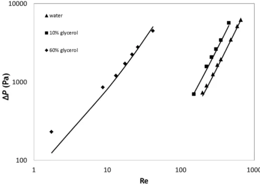
Figure 16 summarizes the pressure drop measurements obtained in the Lab-scale NETmix® 2D and the respective pressure drop model calculations. As explained in section 3.2, four points were taken for each case. The model was fitted to the measured data to

K

=

2.6

, with good accordance regardless of the viscosity or density of the fluid, and all Reynolds number values, except for Re<10, which was tested with 60% glycerine solution. The reason for this deviation may be the higher viscosity of the fluid combined with the limitations of the flowrate and measurement system of the setup. Although the set of data points are in good accordance within them, any possible measurement error at the lowest flowrate of 0.45 ml/s can result in higher deviations from the model.

Figure 16 Plot of pressure drop versus Reynolds number for Lab-scale NETmix® 2D in laminar regime; lines represent pressure drop model with

K

1 f

= −

2log

δ

3.7 d

_h

+

2.51 Re

f













(24)

(30)

19 where

δ

is the surface roughness.

Figure 17 Plot of pressure drop versus Reynolds number for Lab-scale NETmix® 2D laminar and turbulent regimes; line represents pressure drop model for

K

=

2.6

. Dashed line marks the

Re

=

2100

_.

Figures 18 and 19 show the results obtained in the Multi-Inlet NETmix® 2D and the NETmix® 3D prototypes and the respective model predictions fitted to

K

=

12.3

and

K

=

0.8

, respectively. In the case of the Multi-Inlet NETmix® 2D, a centrifugal pump was used to reach the higher

Re

values, it was not possible to obtain measurements for

Re

>

375

. Again in both cases a good fit is obtained between the pressure drop model and the experimental results.

Figure 18 Plot of pressure drop versus Reynolds number for Multi-Inlet NETmix® 2D in laminar regime; lines represent pressure drop model with

K

=

12.3

.

(31)

20 Figure 19 Plot of pressure drop versus Reynolds number for NETmix® 3D in laminar regime;

3.4 Frequency of Oscillation for NETmix®

Above a certain Reynolds number, known as the critical Reynolds number, self-sustained oscillations of the flow field occur inside the NETmix® reactor [4, 7, 17]. These oscillations are considered to be intrinsic to the nature of the flow, not determined by external factors such as variations in the flow velocity caused by peristaltic pump.

(32)

21 1 chamber NETmix chamber q f V

τ

= = (25)

where

q

_chamber is the flow rate through the chamber, and

V

_chamber is chamber volume.

The pressure data series obtained from one of chambers was processed by LabView interface as explained in Section 3.2. Fast Fourier Transforms enabled the analysis of a wide frequency range as well as the separation of oscillations caused by the pump from the ones occurring naturally within chambers. The pump frequency is estimated at 1/10 of the pump rpm, due the presence of six rollers on the peristaltic pump rotor.

Figure 20 shows an example of a processed signal where the peak at frequency 23.5 Hz is induced by the pump while the 15.5 Hz peak is the frequency of NETmix®.

Figure 20 Processed (FFT) signal for Lab-scale NETmix® 2D at

Re

(33)

22

(a) (b) (c)

=

1/

ατ

with

α

=

0.89

. Since

α

<

1

this result may be interpreted as the chambers having dead volumes or using 89% of the chamber volume for energy dissipation. This result should be confirmed using the other NETmix® prototypes, but it was not possible due to equipment limitations, only one setup had port in channels converging into the same chamber.

Nevertheless, from the experimental results it is clear that dynamic pressure measurements can be used to assess mixing dynamics in a NETmix@ reactor, similar procedure was patented for opposed jets mixer at LSRE/FEUP: Reaction Injection Molding with Control of Oscillation and Pulsation. In the NETmix® this flow frequency is the frequency at which flow is directed from one outlet chamber to the other outlet chamber, this is a mechanism that “cuts” the fluids being mixed in small clumps, and as seen in Figure 22 in each chamber the fluids can be cut at frequencies up to 16Hz. Another conclusion from this result is that the frequency of oscillation is fitted by a universal model and is not dependent on the Reynolds number but only on inertial effects: flow rate and reactor volume.

(34)

23 Figure 22 Measured and model frequency data for Lab-scale NETmix® 2D reactor.

Appendices 4, 5 and 6 show the processed signal of the oscillations in Laboratory scale 2D NETmix® geometry, where the appearance and progression of oscillations are visible.

(35)

24

4 T-jets Static Mixer

4.1 T-jets Concept and Description

T-jets mixers are the most popular static mixers in the field of fast chemical reactions [11]. Due to the low mixing times and simple cylindrical shape which enables easy cleaning with a piston, this simple geometry started the reaction injection molding (RIM) process which was invented by Bayer AG in 1964 [22].

First attempts to model the mixing performance in terms of striation thickness were published in 1979 [23]. However, due to the scarcity of released practical data and lack of computing power to simulate the systems, the prediction of parameters was extremely difficult [23].

Recent studies by the aid of computational fluid dynamics and particle image velocimetry, uncovered the chemical reaction behaviour with respect to different flow characteristics [23] as well as hydrodynamics [3]. This hydrodynamic study was also focused on the energy dissipation within the chamber for mixing enhancement however not for comparative purposes.

Most T-jets static mixers in industrial applications have cylindrical shaped chambers and channels [22]. In this work both chambers and channels present are rectangular cross-section prisms, resulting in easier construction of the device, since the mixer can be easily carved from a solid block. Furthermore visualization experiments become readily undertaken by using a transparent top cover (Figure 23a).

The geometric parameters of the T-jets used in this work are shown in Figure 23b. The depth (thickness) is uniform for both channels and chamber and is denoted by

d

. Two other parameters under study are the channel width,

w

_{, and the chamber width,}

W

. The length of the chamber, H, and the chamber head space before the jets inlet,

h

, were kept constant in this work.

(36)

25

(a) (b)

Figure 23 T-jets geometries: (a) photograph (b) schematical view.

4.2 T-jets Experimental Set-Up

For the evaluation of pressure drop behaviour of T-jets mixer, eight different geometries were studied, with the several parameters listed in Table 3. The first three geometries were used to study the effect of the channel width keeping the other parameters constant, while the other five were used to study the depth effect. The two parameters kept constant in all geometries were H =40 mm and h=2 mm.

Table 3 List of studied T-jets reactors geometrical parameters. Geometries Chamber Width , W mm Channel Width , w mm Chamber/Channel Depth , d mm

W w

W d

2 0.5 4

(37)

26 T-jets were mounted on an acrylic carved block with a transparent cover for visualization where a metallic T-jets is inserted as shown in Figure 24. A general scheme and photograph of the experimental set-up are shown in Figures 25 and 26.

Figure 24 T-jets mixer mounted on acrylic block.

Figure 25 General scheme of T-jets experimental set-up.

T-jets setup uses the same kind of differential pressure transducer as in NETmix®. However, no pump is used for T-jets. Instead, two vessels have been used under air pressure to convey fluid during experiment. The installation is controlled from a LabView interface that is shown in Figure 27 and was also used for the data acquisition.

(38)

27 Figure 26 T-jets experimental setup: 1-T-jets, 2-pressure transducer, 3-control valves,

4-pressurized vessels, 5-camera, 6-computer.

The LabView interface (Figure 26) gets the desired Reynolds number and fluid temperature data from the user to calculate required flowrate. The flowrate value is transmitted to the control valves, which set the specified flowrate.

The pressure values are read from the transducer by the LabViev interface and stored to the desired excel file with the corresponding Re value. The Re values can be changed gradually by a knob, directly in an input box or automatically by defining the start and finish Re values and pressing “start”. Automatic mode will increase the Re values by the increments of 10 and wait 10s to start recording data for each new Re value. The block diagram of this interface is shown in Appendix 3.

Figure 27 T-jets LabView interface: 1-input knob, 2-automatic input values, 3-data series record domain, 4-pressure drop value, 5-fluid and geometry parameters, 6- measured flowrate, 7- data

(39)

28

4.3 T-jets Pressure Drop

4.3.1 T-jets Pressure Drop Model

The model for the pressure drop in T-jets mixer is similar to the one used for NETmix® mixer, with

( _channelF 2 _chamberF LF NLF) _channel

P R R R R q

∆ = + + + (26)

The friction resistance contribution is now divided in two terms. For the channel

2

1

2

F channel channel channel h channel

q

L

R

f

d A

ρ

=

(27)

and for the chamber

2 1 2 F chamber chamber chamber h chamber q L R f D A ρ = (28)

where

d

_h and

D

_h are the hydraulic diameters for the channel and chamber, respectively. The linear (viscous) flow resistance term is given by

* 2

1

2

LF channel channel h channel

q

L

R

f

d A

ρ

=

(29)

The

L

* is the distance covered by the jet from its impingement point to the chamber oulet;

*

L = +a b, as shown in Figure 28. Similar to the NETmix® pressure drop model, when the fluid enters the mixing chamber, it is kept as a jet transferring energy to its viscous fluid boundaries, this phenomenon can be observed along the

a b

+

pathline for low Reynolds numbers. When the flow starts to oscillate,

L

* changes, which means getting shorter. However, as this resistance is significant for lower

Re

values, the full

a b

+

length will be used to model this resistance for T-jets.

(40)

29 Figure 28 T-jets scheme showing the calculation of

L

*.

The non–linear flow resistance term is given by

2 1 2 NLF channel channel q R K A

ρ

= (30)

Where K is an adjustable parameter to fit the model to experimental data.

4.3.2 T-jets Pressure Drop Result

Figures 29 and 30 show the effect of depth,

d

, and channel width,

w

, respectively, on the pressure drop. Note that the W6w1d6 geometry could be tested only until

Re

=

550

due to the flow limit of the control valve. As expected, the pressure drop increases with decreasing depth and channel width.

(41)

30 Figure 29 Plot of pressure drop versus Reynolds number for different T-jets depth values; lines

represent the pressure drop model fitted for each geometry.

Figure 30 Plot of pressure drop versus Reynolds number for different T-jets channel width values; lines represent the pressure drop model fitted for each geometry.

The solid lines represent the pressure drop model best fit for each geometry with the respective

K values shown in Table 4 and plotted in Figure 31.

It is observed that K decreases as the depth,

d

, increases and it increases with increasing channel width,

w

. Also higher values of K are observed for the three geometries with larger chamber widths to channel widths ratios, W w/ =1 has the highest K value followed by

/ 2

W w= . The effect of W w/ on K is quite clear with variation of twofold on W w/ the K

(42)

31 effect of W w/ on the values of K is probably the reason of the different values obtained for this parameter between the two 2D NETmix® geometries (see section 3.3.2).

Table 4 Fitted K values for the studied T-jets geometries.

Geometry W6w1d1 W6w1d2 W6w1d3 W6w1d4 W6w1d6 W2w0.5d4 W2w1d4 W2w2d4

K 10.31 8.5 3.35 2.64 1.86 2.39 21.9 88.25

A fourth value of W w/ =6 was studied, in the geometries having W =6mm. The chamber width to chamber depth ratio in the W =2mm geometries was d W/ =2, while in the W =6mm this ratio was in the range 1/6 to 1. For the larger d W/ =1 and W w/ =6, the K value was the smallest of all cases. In an attempt to explain some of these results, CFD simulations of these T-jets geometries were carried out and are shown in Section 4.6.

(a) (b)

Figure 31 Effect of depth (a) and channel width (b) on the fitted values of K.

4.4 Tracer experiments

In order to visualize and study the effect of geometry on flow and mixing, tracer experiments were done and recorded using Orange I (at a very low concentration of 100 ppm to not affect the physical properties) as tracer in one of the jets.

During the experiments it was observed that for the shallower geometries with d =1mm and 2 mm

d = the flow kept segregated up to

Re

=

When the same

W w

/

ratio is applied to a deeper geometry such as W6w1d6, as shown in Figure 33, the oscillations, that start after

Re

=

100

_{, seem more sustainable than the shallow}

geometries. Sustainability of the oscillations means the system does not go back to segregated flow if the flow rate is kept constant.

(a) (b)

Figure 33 T-jets tracer experiments for W6w1d6 geometry: a) segregated flow for

Re

=

150

and b) oscillations for

Re

=

300

.

For geometries with d>2 mm, once the segregated flow steady state is lost

Re

=

140

, the system does not return to the non-oscillating segregated flow. With these geometries, as

Re

increases the oscillations’ frequency and amplitude increases intensifying the chaotic advection.

(44)

33

4.5 T-jets Energy Dissipation

Siddiqui et al. reported [24] energy dissipation terms from kinetic energy balance and pressure drop measurements. Model equations can be given as follows

2 pressure mixer q P V

ε

ρ

∆ = (31) 2 total mixer q P KE V

ε

ρ

∆ + ∆ = (32)

where V is the total volume of the mixer and RKE is defined as;

2 2

channel chamber

KE mv mv

∆ = − (33)

Energy dissipation of T-jets were calculated from experimental pressure drop data and are shown in Figure 34. These results enable the comparison with the SMV mixer’s energy dissipation of 793 W kg/ , introduced in Section 2.2.4. Considering the trendline of W2w2d4 geometry’s energy dissipation data which can be shown as;

ε

_total

=

Re

2.4332

10

5 (34)

it can be concluded that, to achieve the same level of energy dissipation, the SMV mixer has to operate in turbulent regime [11], whereas the W2w2d4 geometry theoretically dissipates 793 W kg/ at

Re

=

1764

.

(45)

34 To benchmark the SMV with T-jets, energy dissipation would not be enough. Power number needs to be incorporated to this comparison.

4.6 T-jets CFD Simulations

Computational fluid dynamics is a powerful tool, extensively used for both static and agitated mixers in the past [25]. The most commonly used model within this area of static mixer is the finite volume as well as finite elements and Boltzman lattice methods. Mixing time, mixing quality, heat transfer and pressure drop have been studied with this method [11, 25].

For NETmix®, CFD modeling plays a special role since the idea of network mixing reactor was developed first using CFD [7]. The model was then applied to practice and validated. Critical Reynolds Number, after which the reactor starts to validate the model of perfectly mixed chambers, were investigated and reported.[17]. 2D CFD studies were also conducted in order to simulate the mixing mechanisms for a wide range of Reynolds number [18].

For T-jets mixers, although the 2D model was proven valid for the mixing assessment [26], 3D simulations were also made. CFD simulations were previously used to study the effect of jets momentum imbalance in the ﬂow ﬁeld of opposed jets reactors by Johnson [23] and simple opposed jet geometries were successfully tested by CFD [27].

In this work different channel to chamber ratios and different depths were studied in order to find out which parameters affect the K values.

4.6.1 CFD Model

The T-jets geometry was modelled by the aid of ANSYS Design Modeler, MESH. After the design of geometry, the channels and the chamber were separated to be meshed with uniform all quad face elements. An example of the final mesh for 6 mm chamber width, and 1 mm channel width is shown in Figure 35.

(46)

35 After constructing the mesh, Fluent 13 was used to set up the simulation case. For all the simulations the case and mesh conditions are given in Table 5.

Table 5 CFD model used for the 2D T-jets simulations

Case Parameter Setting Observations

Mesh Parameters

mesh geometry 2D -

face size 0.1mm 10 cells refinement

between channel walls

mesh method uniform quad -

Inlet left velocity inlet -

Inlet right velocity inlet -

outlet pressure outlet -

Case Parameters

walls no slip - aluminium -

fluid pure water Density = 998kgm

-3

Viscosity=0.001003kg/ms

models viscous-laminar -

solution methods

SIMPLE Least square cell

based

Second order - Upwind

initial solution achieved with first order, then

enhanced

inlet velocities 0.05m/s Re = 50

4.6.2 Effect of Depth in T-jets Geometry

In Section 4.3.2 the K values with respect to the depth of geometry were given in Figure 31, where it could be observed an asymptote for d >2 mm. This fact suggests that geometries shallower than 2 mm would have a different mechanism than the deeper ones.

This mechanism can be interpreted as a deviation from the 2D flow mechanism due to strong wall effects in shallow chambers. In other words, the flow in shallow chambers is more affected by 3D effects, namely rotation of flow having rotation axis aligned with the direction of the chamber axis, these flow regimes are called as vortex or engulfment flow [28-29]. For deeper chambers the main flow structures are vortices that rotate in the normal direction to the chamber axis. Here 3D effects, namely rotation of flow with rotation axis aligned with the direction of the chamber axis, are not so dominant. These flow regimes are called chaotic flow. This theory was studied qualitatively by transient 2D CFD simulations. Velocity contour plots are shown in Figure 36 for a W6w1 geometry where the 2D flow mechanism that give rise to the oscillations seen in the tracer experiments (Figure 33b) are observed.

(47)

36 Figure 36 Velocity contour plot for transient 2D simulation of W6w1 for

Re

=

300

_.

4.6.3 Effect of Channel Width in T- Jet Geometry

It was observed previously that the K factor increased as the channel width increased. This fact was somehow contradictory to the initial theory due to the decreasing

W w

/

ratio. 2D simulations of geometries W4w0.5, W4w1 and W4w2 were made in order to further investigate this. The simulation results are shown in Figure 36. It was observed from streamline data that as the inlet channel diameter increases, the laminar jet flowing through the centre of the chamber occupies a larger part of the chamber width, thus there is less space for the formation of vortices between the jet and the chamber walls. This would naturally result in higher pressure drop, and thus friction was lower for wider channels. Although the pressure drop due to friction was lower, the nonlinear flow contribution was enough to yield higher values of K.

(a) (b) (c)

Figure 37 2D streamlines for steady state simulations for different geometries at

Re

=

50

: a) W4w0.5; b) W4w1; c) W4W2.