Equity valuation research : Corticeira Amorim SGPS S.A.

Equity Valuation Research:

Corticeira Amorim SGPS S.A.

Tomás Sousa de Carvalho, 152110316

Advisor: Professor José Carlos Tudela Martins

Dissertation submitted in partial fulfillment of requirements for the degree of MSc in Business Administration, at Católica Lisbon School of Business and Economics, 16th of September 2013

Page | i

ABSTRACT

Equity Valuation Research: Corticeira Amorim SGPS SA

by Tomás Sousa de Carvalho

The main objective of Equity Valuation is to measure the value of a company based on its current assets and market position. The use of Equity Valuations help investors to make most informed investment decisions taking into account the true value of a company at any given time and its expected performance in the future. Notwithstanding, a good valuation must be based on consistent and solid assumptions in order to provide the most reliable illustration of the company business reality. In this sense, a proper equity valuation analysis needs to address all the critical endogenous and exogenous factors that influence the company business. The chosen valuation approach will also determine the accuracy of the final results.

This dissertation focus on the Equity Valuation of Corticeira Amorim SGPS SA, the world’s biggest cork-transforming company and one of the most international Portuguese companies. In a period of unfavorable economic context, Corticeira Amorim has been able to buck the negative trend of most Portuguese companies based on its sustainable growth. Thereby, the company seems to be an interesting investment target to investors considering the recent and future optimistic perspectives of its business. Hereupon, the objective of this dissertation is to provide an investment recommendation based on the estimated market value of Corticeira Amorim. Throughout this dissertation, all the determinant topics that support the valuation results are discussed, namely: different valuation approaches, industry and company overviews and forecast assumptions. The final topic focus on the comparison between BPI bank and this dissertation analyzes, discussing the differences on both valuations.

Page | ii

ACKNOWLEDGEMENTS

This dissertation represents the last chapter of my academic life and the final product of my hard work during the past few months which I would not be able to accomplish without the help and support of some people throughout this journey. I would like to express my sincere gratitude to all these people.

Firstly, I want to thank all my family for their motivation, support and encouragement during this period of my life, especially to my parents, Graça and Bruno. Their love and faith helped me to complete this critical challenge of my life. I would also like to thank my grandfather for representing the role model I tried to follow during all my academic life as a student and most importantly, as a person.

I would like to gratefully thank Professor José Tudela Martins, for all his availability, guidance and patience during these last two years of studies, firstly as my teacher, then as my thesis advisor. Moreover, I would also like to thank Dr. Álvaro Santos and Dra. Madalena Santos, for giving me the opportunity to write my master thesis about Corticeira Amorim. Their availability in answering all my questions and providing me all the information I needed, were a great surplus to the final outcome of this dissertation.

I would also like to thank all my friends, especially Diogo and Gonçalo, for their true friendship during this last few months. They were the two people I most shared time with, either in University or in each others’ homes. Their company, encouragement and comfortable words represented a great motivator to me throughout this process. Finally, and most importantly, I would like to thank my girlfriend Constança for her support, patience and friendship which helped me overcoming the most tough obstacles I had to face lately. Without her support I would not be able to finish my dissertation.

Page | iii

Table of Contents

0. Introduction

1

1. Literature Review………...2

1.1.

Valuation Approaches………...2

1.2.

Discounted Cash Flow (DCF) Valuation ………..………...….3

1.2.1. Free Cash Flow to the Firm (FCFF) Model……….……….……..…..4

1.2.1.1.

Variables of the FCFF Model………..……….…………...5

1.2.1.2.

Value of the Firm………..………...7

1.2.1.3.

Terminal Value……….…...….8

1.2.2. Weighted Average Cost of Capital - WACC……….……….…..10

1.2.2.1.

Cost of Equity………12

1.2.2.2.

Risk free rate……….13

1.2.2.3.

Equity Beta……….14

1.2.2.4.

Equity risk premium………16

1.2.2.5.

Cost of debt………..17

1.2.2.6.

Weights of debt and equity………..18

1.2.2.7.

Small Cap discount………..19

1.3.

Relative Valuation………..………..20

1.3.1. Price Earnings ratio – PER………..….22

1.3.2. Enterprise Value to EBITDA………...23

1.3.3. Relative vs. DCF Valuation………..23

2. Company Overview………..…….24

2.1.

Global Information………24

2.2.

Business Activity……….25

2.3.

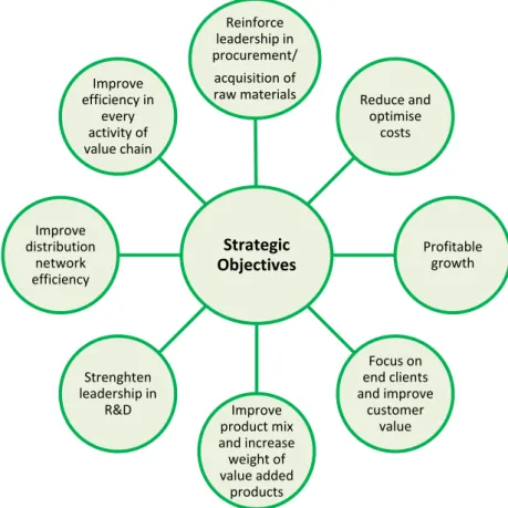
Strategic orientation and future objectives………26

Page | iv

3. Cork Industry Overview……….……….31

3.1.

International market for cork……….……….….31

3.2.

Portuguese market for cork……….…..……32

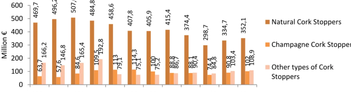
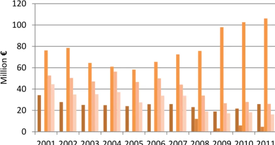
3.2.1. Cork exports………...……..32

3.2.2. Cork imports……….….36

3.3.

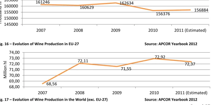
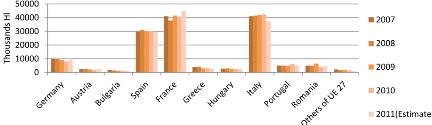
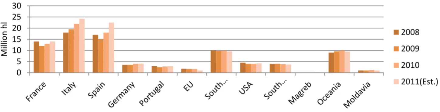
Wine Industry………...……37

3.4.

Cork related industry trends and market outlooks………..39

3.4.1. Wine and Spirtis market………39

3.4.2. Construction and Building materials industry………..39

4. Methodology……….………..…..40

5. Forecast assumptions……….………..…..41

5.1.

Revenues of business units……….…………41

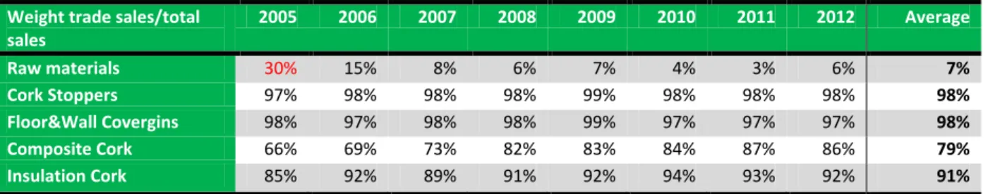
5.1.1. Raw Materials……….……….42

5.1.2. Cork Stoppers………43

5.1.3. Floor & Wall Coverings……….……...….44

5.1.4. Composite Cork……….……….…….44

5.1.5. Insulation Cork……….……….……..45

5.1.6. Other considerations………..46

5.2.

Operating expenses and other operating income……….46

5.3.

Gross PP&E, Intangible assets and Investment property……….47

5.4.

Depreciation……….………..………..48

5.5.

Net PP&E, Intangible assets and Investment property………..49

5.6.

CAPEX……….……….………49

5.7.

Working Capital………..….……….…..….……….50

5.8.

Cost of Equity……….………..….……….………....51

5.8.1. Risk free rate……….………..….……….………...…………..51

Page | v

5.8.3. Market risk premium………..52

5.9.

Cost of debt……….……….……….……….53

5.10. Weights of equity and debt……….54

5.11. Corporate tax rate………..55

5.12. Terminal Value………..55

6. Enterprise Value of Corticeira Amorim business units……….56

7. Dividends to shareholders of Corticeira Amorim……….………..….…58

8. Debt and Financial costs……….58

9. Retained earnings and non-controlling interests……….59

10. Equity Valuation of Corticeira Amorim………...60

11. Relative Valuation………60

12. Sensitivity Analysis………...….62

13. Dissertation vs. Investment Bank (BPI) Analisys………..63

14. Conclusion………....64

Appendices………...65

Appendix 1: Literature Review – Alternative Valuation Methods……….….65

Appendix 2: History of Corticeira Amorim………...79

Appendix 3: Corticeira Amorim detailed business structure and international presence….…80

Appendix 4: Recent performance of Corticeira Amorim by BU……….81

Appendix 5:Macroeconomic Framework………83

Appendix 6: Cork related industry trends and market outlooks………..87

Appendix 7: Corticeira Amorim business units Overview……….………89

Appendix 8: Operating expenses and other operating income……….98

Appendix 9: Historical values of gross and net fixed assets, depreciation, CAPEX and net

working capital………...102

Appendix 10: Enterprise value of Holding (non-operational BU)………...….107

Appendix 11: Historical dividends to shareholders of Corticeira Amorim……….108

Page | vi

Appendix 13: Historical values of retained earnings and non-controlling interests……..…...111

Appendix 14: Fundamentals of Relative valuation………..112

Appendix 15: Sensitivity Analysis………...115

Appendix 16: Disserattion vs. Investment Bank (BPI) Analysis………..…116

Appendix 17: Income Statement of Corticeira Amorim………...121

Appendix 18: Balance Sheet of Corticeira Amorim………...122

Appendix 19: Cash-flow Statement of Corticeira Amorim………...123

Appendix 20: BPI Investment Report of Corticeira Amorim – Information………..…..124

Page | 1

0. Introduction

The main purpose of this dissertation is to estimate the year 2013 target price per share of Corticeira Amorim SGPS SA, a portuguese holding company listed on the Lisbon Stock Exchange and the world’s leading player in the cork industry. Corticeira Amorim is responsible for the core business of Amorim Group which is majorly hold by the Amorim Family. The major goal of the equity valuation analysis presented in this dissertation is to predict the market value of Corticeira Amorim and consequently its market price per share in order to provide an investment recommendation to current and potential investors of the company.

Nowadays, portuguese companies are facing extremely difficult economic and financial conditions mainly due to the current sovereign debt crisis of Portugal. The tough macroeconomic environment Portugal is living, has been affecting negatively most portuguese companies. Nonetheless, some companies have been registering very positive results despite the unfavorable context and Corticeira Amorim is a great example of that. With a very strong global presence in the most important construction and wine markets, Corticeira Amorim has been able to expand its cork business and strengthen its position as the world’s leading company in the cork industry. The variety of segments where the company operates and its worldwide global presence has been allowing the company to grow consistently, controlling the business risks and somehow, overcoming the difficulties.

Corticeira Amorim is divided into five business divisions: Raw Materials, Cork Stoppers, Floor & Wall Coverings, Insulation Cork and Cork Composites. Holding a vast number of companies and subsidiaries, Corticeira Amorim is world leader in every cork segment where it is present. The equity valuation in this dissertation estimates separately the enterprise value of each business unit and then add them together in order to get the consolidated enterprise value of Corticeira Amorim.

The structure of this dissertation is organized into four major sections. Firstly, it is presented the Literature Review which explains in detail the most important Equity Valuation models and their applicability. The second section is related with the company and industry overview, analyzing the historical information of the cork, construction and wine industries in order to contextualize Corticeira Amorim cork business. The third section presents the Equity Valuation of the company and its five business units using the Discounted Cash Flow model complemented by a Relative Valuation. Finally, the results are compared with the ones of BPI Equity Research in its annual investment report to investors, discussing the different assumptions and results obtained in both valuations.

Page | 2

1. Literature Review

1.1. Valuation Approaches

As Damodaran (1996) states “Valuation can be considered the heart of finance”, given the great importance it has in helping managers to make sensible decisions. Valuation seems to be a very powerful tool for managers in analyzing the potential decisions to make in most financial fields of study. The assessment of investment, financing and dividends decisions in corporate finance, the estimation of the true value of a stock in portfolio management or its market price trend in empirical finance, are good examples of how important is valuation in achieving the ultimate goal of managers, the value creation.

In the business context of a firm, “the managers’ ability to estimate value is a critical determinant of how the company will allocates its resources” (Luehrman, 1997). In turn, according to Luherman (1997) “the allocation of resources is a key driver of a company’s overall performance”, that is why valuation assumes such a preponderant role on the regular resource-allocation decisions of general managers. In order to make a recommendation and explain why this valuation brings value added to potential investors, the focus of this dissertation is on the price per share of Corticeira Amorim SGPS

SA, which reflects its equity value.

From all the models usually used in firm valuation, the WACC-based DCF (Discounted Cash Flow) is the one that most companies use to value their corporate assets. This model consists in “valuing the business according to its expected future cash flows discounted to present value at the weighted-average cost of capital of the firm” (Luehrman, 1997). Despite being the most generic model in firm valuation, there are different types of valuation problems which may require distinct analytical challenges and approaches from the WACC-based DCF.

According to Luehrman (1997), managers need to address three different valuation problems: valuing operations, opportunities and ownership claims. The author states that the Adjusted Present Value (APV), the Option Pricing and the Free Cash Flow to Equity (FCFE) are the most suitable models for each type of problem, respectively. The main difference among these valuation methods is expressed in the nature of the cash flows used in the value estimation.

Page | 3 Generally, there are four approaches in firm valuation (Damodaran, 2006): the Discounted Cash Flow

valuation, already mentioned, the Asset-Based valuation, the Relative valuation and the Contingent Claim valuation. The Asset-Based valuation usually values the existing assets of a firm through

accounting estimates or book value, the Relative valuation estimates the value of the assets by looking at the pricing of comparable assets in the market and some of the firm’s variables like earnings, sales, book values or cash flows, the Contingent Claim valuation values the assets that share option characteristics using option pricing models.

According to the overall characteristics of Corticeira Amorim SGPS SA, the Discounted Cash Flow method is the most suitable approach taking into account the company’s “big picture”. The valuation analysis in this dissertation is mostly based on this method and complemented with the Relative valuation approach, in order to test the consistency of forecasts. Despite using only these two approaches in this dissertation, all the previous referred valuation approaches and respective models are also discussed in Appendix 1.

1.2. Discounted Cash Flow (DCF) Valuation

From all the firm valuation approaches, the Discounted Cash Flow valuation seems to be the most consensual among the critics, emerging in the last few decades as the best practice for valuing corporate assets. This valuation approach consists in a simple relationship between the present value and the future (expected) value from the firm’s corporate assets. The basic logic of Discounted Cash Flow valuation is to determine the present value of the corporate assets by discounting the forecasted expected future cash flows on the same assets at the opportunity costs of funds, depending on the discount rate. Both expected future cash flows and discount rates require a few set of assumptions which will determine the accuracy of the valuation.

Taking in consideration the underlying uncertainty involved in the firm’s assets, the expected future cash flows are forecasted according to future growth rates expectations assumed by managers. The discount rate is associated to the opportunity cost of the company, representing the return its owners expect to earn on an alternative investment implying the same risk (Luherman, 1997). The discounted rate is simply “the return investors expect to earn on a risk-free investment for a period of time, plus the risk premium, which reflects the extra return they can expected from bearing a certain level of risk” (Luherman, 1997).

Page | 4 The same logic applies to all the different Discounted Cash Flow valuation methodologies, regarding the relationship between present value and future value of cash flows generated from the firm’s assets. The differences among them are the cash flow components, discount rates and tax effects associated to each specific method. From all the Discounted Cash Flow models used, the most commonly used are the Free Cash Flow to the Firm (FCFF), the Free Cash Flow to Equity (FCFE) and the Adjusted Present Value (APV) method, which are going to be discussed in this chapter. Other DCF valuation method addressed in this discussion is a FCFE variant, the Dividend Discount model, as well as alternative approaches like the Excess Return models.

1.2.1. Free Cash Flow to the Firm (FCFF) Model

According to Damodaran (2006), there are two ways of approaching the Discounted Cash Flow valuation: either valuing the entire business of the company with both assets in-place and growth assets (firm/enterprise valuation) or valuing the equity stake in the business (equity valuation). The value of the equity can also be obtained through the first approach by netting out the value of all non-equity claims from the firm value. If the valuation estimates are based in consistent assumptions and correctly calculated, the value of the equity must be the same in both cases.

In the firm valuation approach, the Free Cash Flow to the Firm or WACC-based Free Cash Flow (FCF) analysis is considered by many the best valuation method regarding the valuation of corporate assets or at least, the most consensual among the financial academia. In the last few decades, this particular methodology of the Discounted Cash Flow valuation emerged as the best practice for companies in their capital-budgeting process due to its simplicity, being relatively intuitive and easy to learn. The major advantage of using the firm valuation approach compared to the equity valuation approach is explicitly expressed in cases where the leverage is expected to change significantly over time. Being a pre-debt cash flow, the FCFF does not need to consider the cash flows related to the debt, being very useful to apply in cases of leverage variation over time, regarding new debt issues and debt repayments (Damodaran, 2006). Although it does not take in consideration debt related cash flows, the use of the FCF method addresses the firm’s debt ratios and interest rates in order to estimate the weighted average cost of capital.

According to Froot (1997), the Free Cash Flow to the Firm may be defined as “after-tax earnings before deductible financing charges such as interest expense, lease rentals and so forth (…) plus all deductible

Page | 5 non-cash charges (e.g., depreciation, deductible amortization, deferred taxes, etc.) and less new cash outlays for required capital expenditures and investment in net working capital”. Basically, it represents the cash flows available to all the financial investors of the firm.

The formula of the FCFF is given by:

FCFF = EBIT*(1-Tax rate) + Depreciation - Capital Expenditure - ∆Working Capital

1.2.1.1. Variables of the FCFF model

In firm valuation, the value of a company reflects not only the value of its assets but also the present value of the forecasted expected cash flows generated by the same assets. Bearing in mind the future perspectives and expectations taken into account when valuing a firm, the assumptions made for each of the variables turns out to be critical to determine the FCFF model accuracy and effectiveness. As Janiszewski (2011) states, “the financial projections of the valued entity should be based on independent factors that have material impact on the company financial performance”. The author considers that an in-depth analysis of the relevant variables affecting financial performance and the correct selection of the key drivers are the two necessary elements of an appropriate DCF approach. These two elements will determine the FCFF model accuracy, so it is critical to understand the different forecast performance methods for each of the variables in order to support the financial projections.

According to the period of time determined for the valuation given the company future prospects, the

EBIT (Earnings Before Interests and Taxes) is forecasted for each period, usually on annual or

semester basis. The EBIT calculation is based on the firm’s operating revenues minus its operating expenses, before deducting interest payments and income taxes. The estimates for the EBIT in each period will be determined by the growth rates assumed for operating revenues and expenses. The macroeconomic, industry and business information are the three main factors that should be considered in the growth rates assumptions, given the expectations and perspectives of the firm (Janiszewski, 2011).

Regarding the tax rate used in the FCFF computations, there are two options: the marginal tax rate or the effective tax rate. The marginal tax rate is the incremental tax the firm has for an additional dollar on its income whereas the effective tax rate is based on actual taxes being paid, taxes due/taxable

Page | 6 income. Usually the effective tax rate is the most commonly used but it is correct to use any of the two, as long as the after-tax cost of debt computation for the WACC is done using the same tax rate.

In order to forecast the depreciation for future time periods, there are three possible options (Koller et al, 2005). The first option is to forecast depreciation based on depreciating methods and policies set out by the company. This approach only makes sense when insight detailed information is available, given that equipment purchases and depreciation schedule of the company are usually the main forecast drivers. There is also the option to estimate depreciation as percentage of revenues or a percentage of property, plant and equipment (PP&E). Koller et al. (2005) defends that using these two options is indifferent in cases where the CAPEX projections are steady over the time, due to the fact that depreciation is directly related to CAPEX, the capital expenditures incurred in fixed asset purchases. When large CAPEX fluctuations are predicted, the best option is to estimate depreciation as a percentage of PP&E, since the value of fixed assets will depend on the CAPEX values.

The CAPEX (Capital Expenditures) are investments made regarding the purchase of new physical assets like PP&E or investments to upgrade the useful life of the firm’s existing capital assets. Sometimes represented as Net Capital Expenditures (CAPEX – Depreciation), it reflects the growth expectations of a firm, typically much higher in high growth firms than low growth firms. The most common methods to predict CAPEX for future periods are based on the firm’s historical accounting data or the reinvestment rates of peer companies, by industry group (Damodaran, 2002). In this last one, the reinvestment rate is given by the average ratio CAPEX/Depreciation of the peer companies by industry. It represents how much companies are reinvesting their earnings on corporate assets to generate future growth. Keeping this in mind, the use of reinvestment rate as a proxy for CAPEX forecasts is more reliable when valuing high growing firms. Damodaran (2002) also presents the use of other possible average ratios (by industry) like Net CAPEX as a percentage of sales or earnings as alternatives to estimate future capital expenditures.

The operational working capital represents the difference between current assets and liabilities. It reflects the ability of the company in meeting current obligations and to expand without recurring to debt financing. A negative working capital traduces the problem of the company in paying back to its creditors in the short term. To forecast the operational working capital, all the items which it depends on have to be forecasted as well. Current operating items like accounts receivable, inventories, accounts payable, accrued expenses, net PP&E and goodwill have to be forecasted in order to

Page | 7 compute the operational working capital. According to Koller et al (2005) the best driver to forecast these items is revenue, meaning all these items should be forecasted as percentage of revenues. Items like inventories and accounts payable might also be forecasted as percentage of costs of goods sold (COGS). Nonoperating items such as excess cash, short-term debt and dividends payable should be excluded from calculations.

1.2.1.2. Value of the firm

Under the FCFF model scenario, the value of the firm is given by discounting the expected future cash flows to the firm at the weighted average cost of capital (WACC). According to Damodaran (2006), when a firm is growing at a steady state, predicted to sustain in perpetuity, the enterprise value (operating assets) is given by:

The FCFF represents the expected free cash flow in the first year forecast and g the assumed growth rate in perpetuity.

The author argues that are two major conditions regarding the growth rate assumptions that have to be respected when using this model, also applicable to FCFE and dividend discount models. The first condition imposes that the assumed growth rate used in the valuation cannot be bigger than the growth rate in the economy, either in nominal and/or real terms. The second one is related to the fact that reinvestment rates assumed for the expected free cash flows to the firm have to be in harmony with the firm’s growth rate assumption; otherwise changes in capital expenditures relative to depreciation will have a negative correlation in these same cash flows, contradicting the growth assumption previously mentioned. The two main drivers of the growth rate should be the company’s business growth strategy (e.g.: acquisitions, product innovation, R&D, etc.) and the industry/markets where the company operates (Koller et al., 2005).

After computing the value of the firm operating assets, there are adjustments needed to be done in order to get the final equity value of the firm. Although having direct impact in the enterprise value, the non-operating assets are not taken into account in the FCFF forecast. These assets “represent all the assets whose earnings are not counted as part of the operating income” (Damodaran, 2006), that

Page | 8 have to be added to the value of the company operating assets in order to get the real enterprise value /the value of the firm assets. Excess cash, marketable securities and minority holdings in other companies are some of the most common non-operating assets that need to be considered in the final enterprise valuation. Finally, in order to get the final equity value of the firm, all the non-equity claims have to be subtracted from the adjusted enterprise value. Non-equity claims are mostly composed by net debt and minority interests (market value) as well as underfunded/overfunded pension liabilities, capitalized leases and some special dividend payments.

1.2.1.3. Terminal Value

The terminal value or continuing value is the discounted value of the expected future cash flows generated by the firm after the financial projections period. According to Damodaran (2012) there are three ways to estimate the terminal value: the liquidation value approach which basically represents the market value of the firm in the terminal year, the multiples approach which relies on multiples from comparable firms and is not applicable to discounted cash flow valuation and the stable growth model approach. The first two approaches are not going to be used in this dissertation.

Focusing on the stable growth model, the terminal value estimation relies on a steady long-term growth perpetuity assumption that will have a direct impact on the value of the company, since it represents the majority of the final firm value. Therefore, assumptions related to the expected long-term growth rate in perpetuity need to incorporate not only the company future perspectives but also the industry and economy expectations, in order to get accurate and reliable firm value estimations. In cases where a zero long-term growth is assumed, it is implicit that the firm will earn its cost of capital on all new investments into perpetuity (Janiszewski, 2011).

Under the stable growth model approach, there are some constrains implied in the long-term growth rate estimation which need to be taken in consideration in order to get an accurate terminal value and firm value (Damodaran, 2012). Besides, the growth rate limited value imposed by the economy where the company operates, Damodaran points out two other important constrains which may affect the estimation rate. The adjustments in the stable growth rate have to be in accordance with the currency being used to estimate cash flows and discount rates. The author alerts that higher growth rates are expected for high-inflation currencies and lower growth rates expected for low-inflation currencies “since the expected inflation rate is added on to real growth”. The other constrain is also related to the

Page | 9 fact of expecting higher/lower growth rate estimations depending on the nominal/real term valuation being done, respectively. Kaplan and Ruback (1995) also highlight the importance of adjustments related to capital expenditures and depreciation in the last forecasted year. Both authors defend that capital expenditures should equal depreciation in the last forecasted year to eliminate the inconsistency regarding the difference between these two elements. The logic behind this assumption is the fact that firms will only reinvest enough funds to replace the value of their assets, in the long term.

The formula to estimate the terminal value using the stable growth model, under the FCFF approach is given by:

Assuming that the firm “will continue to reinvest some of its cash flows back into new assets and extend their lives” (Damodaran, 2012). FCFF n+1, represents the expected cash flow to the firm one year following the terminal year, WACC the weighted cost of capital and the constant growth rate

in perpetuity. The same formula is applicable to the FCFE and Dividend Discount model context, depending on the cash flow nature used in the valuation.

Having the terminal value calculated, the value of the operating assets of the firm is given by:

∑

The first period corresponds to the present value of cash flows during explicit forecast period and the second period to the present value of cash flows after the explicit forecast period, representing the terminal value.

An important aspect that affects the terminal value and the value of the explicit period is the forecast horizon assumed in the valuation, represented by n in the formula above. Koller et al. (2005), state that the length of the explicit period forecast does not affect directly the firm value but it will affect the “distribution of the company’s value between the explicit forecast period and the years that follow”. The longer the explicit forecast period is the less weight the terminal will have on the total

Page | 10 firm value. According to the authors, when changes in economic assumptions related to the terminal value estimate are expected, the forecast horizon affects indirectly the firm value. This is explained by the excess value of the return on invested capital (ROIC) over the cost of capital of the firm during the explicit forecast period, since it is commonly assumed that both values are equal during the continuing value period. The appropriate length of the forecast explicit period should be equal to the period when the company reaches a steady state regarding its growth, margins, capital turnover and WACC (Koller et al., 2005), otherwise the terminal value estimate will not be useful. In order to set an appropriate forecast horizon, Janiszewski (2011) points out the length of high growth/transition growth period, the industry cycle and competitive structure (operating margins), the economic cycle and the length of any competitive advantage as the main drivers of the explicit forecast period. Although there is no specific limit to the forecast length period, authors like Ohlson and Xiao-Hun Zhang (1999), defend that explicit forecast period should never surpass 15 years.

1.2.2. Weighted Average Cost of Capital – WACC

Over the last decades, the most common technique used in the discounted cash flow valuation approach is the WACC-based DCF analysis. According to this DCF method, “the value of a business equals its expected future cash flows discounted to present value at the weighted-average cost of capital” (Luherman, 1997). Koller et al. (2005) refer that “the WACC represents the opportunity cost that investors face for investing their funds in one particular business instead of others with similar risk”. Usually companies use two sources of financing to fund their businesses, either through equity or debt, and sometimes hybrid securities. Given that free cash flows represent the cash flows available to all the financial investors of a company, the WACC have to incorporate the required rates of return of equity and debt holders, expressed in the market cost of equity and after-tax cost of debt, respectively. Therefore, the opportunity cost of capital is obtained by adding the weighted market cost of debt and equity according to the proportional claim of each funding source in the capital structure of the company.

When valuing leveraged firms, the WACC computations must be done in after-tax terms in order to capture the value of tax shields by using debt, in the cost of capital. This value represents the tax benefits available from interest expenses tax exemption which is not included in the FCFF calculations, thus it has to be incorporated in the cost of capital. As Froot (1997) states, “ by employing the after-tax cost of debt in the weighted average, the tax advantage of using debt to finance the investment is

Page | 11 automatically captured in the discounted-cash-flow analysis”. In general terms, the weighted-average cost of capital formula is given by:

( ) ( )

As the formula suggests, the WACC calculation relies on three components that need to be estimated: the market after-tax cost of debt (Kd*(1-tc)), the market cost of equity (Ke) and the weights of debt (D/V) and equity (E/V) regarding the enterprise value (in target values). The marginal corporate tax rate is represented by tc (Koller et al., 2005).

Usually, the WACC is calculated assuming that companies will set a target optimal capital structure over time. As explained before, the use of debt as source of financing allows the company to increase its value until a certain point, capturing the value of the interest tax shields. The bigger the debt weight is, the smaller will be the cost of capital of the company, until the point where the positive value of interest tax shields is offset by the negative value of expected bankruptcy and agency costs related to an excessive debt weight. Hence, this point represents the optimal financing mix which is assumed in this particular model in order to maximize the enterprise value.

Although it is commonly seen as a simple, robust and intuitive valuation method among the financial academia, some critics point out drawbacks in the WACC-based DCF analysis. Miles and Ezzel (1980) argue that a constant capital structure over time is not realistic most of the times; therefore the model is not always reliable. Luherman (1997) also criticizes the capacity of the model to handle with “all the adjustments required by a complex capital structure, since the WACC is a tax-adjusted discount rate built to pick up the tax advantage associated with corporate borrowing for a simple capital structure”. The author also questions the “fairly restrictive assumptions” which WACC relies on regarding complex tax positions, which may lead not only to the “misevaluation of the interest tax shields but also other cash flows associated with projects and its financing”.

On the other hand, Damodaran (2006) defends that the WACC approach does not require the assumption of a constant debt ratio, stating that “the approach is flexible enough to allow for debt ratios that change overtime”. In fact, according to the author the model flexibility is one of its biggest strengths given that changes in the financing mix “can be built into the valuation through the discount rate rather than through the cash flows”.

Page | 12

1.2.2.1. Cost of Equity

Being part of the weighted average cost of capital, the cost of equity is commonly used by managers as hurdle rate in investment-related decisions. Since it is impossible to predict with total certainty the expected rates of return from investments, usually financial managers rely on asset-pricing models to estimate those same returns which are translated in risk. The most common used asset-pricing model to estimate expected returns and determine the cost of equity of a company is the Capital Asset Pricing Model (CAPM), which defines the cost of equity as the expected return on a company’s stock.

According to Mullins (1982), the model assumes that “a stock’s expected return is the shareholder’s opportunity cost of the equity funds employed by the company”, explaining that the cost of equity is the minimum return a company must expect on the “equity-financed portion of its investments”. In cases where this condition is not valid, the author argues that the company should invest in other securities with the same risk level in the financial marketplace otherwise the stock price of the given stock will deteriorate.

The main insight acknowledged by the model is the fact that market risk is the only relevant variable that affects equity-related investments and consequently their expected rates of return. Since the model assumes all investors are sophisticated well-informed and risk-averse, the diversifiable or unsystematic risk is eliminated through simple portfolio diversification, being the systematic/market risk the only risk investors are exposed to (Mullins, 1982). Therefore CAPM’s objective is to estimate the expected return on investments described by the market behavior, represented by the security market line (SML) which reflects the risk/expected return relationship. By definition, the SML will also provide estimates of cost of equity given by:

Cost of Equity = Risk-free rate + Market Premium x Beta

In order to determine the cost of equity, the risk-free rate, the expected return on the market and the beta need to be estimate. According to Koller et al. (2005), the beta is the only of the three variables that varies across companies. The authors define beta as “the stock’s incremental risk to a diversified investor, where risk is defined by how much the stock covaries with the aggregate stock market”. The stronger the correlation between the stock and the aggregate market is, the higher the beta will be and vice-versa.

Page | 13 Despite being widely used in estimating the cost of equity, CAPM’s assumptions suggest some critics regarding its applicability. Mullins (1982) argues that a complete elimination of the unsystematic risk is impossible given that perfect negative relationship between the returns of two stocks is very rare in real markets. The fact postulated by CAPM that only systematic risk matters, is criticized by the author, arguing that most of the investors “do not hold adequately diversified portfolios”, leading them to be compensated with” higher expected returns for bearing only market-related risk”, which may not be in accordance with the empirical evidence. Other underlying assumption of the model concerning a market with no imperfections like transaction costs, taxes and restrictions on borrowing and lending, are unrealistic to the author given the real behavior of the complex financial markets. Fama and French (1999) point out “empirical failures of the CAPM due to bad proxies for the market portfolio” because they are not mean-variance-efficient unlike the true market. Despite some criticism about its shortcomings, CAPM seems to be the most consistent model to estimate the cost of equity. As Mullins (1982) states, “CAPM’s deficiencies appear no worse than those of other approaches (…) Its key advantage is that it quantifies risk and provides a widely applicable, relatively objective routine for translating risk measures into estimates of expected return”.

Alternatively to asset-pricing models, namely the CAPM, the Dividend Growth model or Gordon-Shapiro model is other approach used to estimate the cost of equity. This model is a simple discounted cash flow technique which demonstrates that the price of a company’s stock equals the present value of future dividends per share discounted by the cost of equity capital (Mullins, 1982). The main constrain of the model is related with the assumptions related to perpetual growth rate in dividends per share that cannot be higher than the cost of equity. Thus, the model excludes companies with unsteady dividend payments and high growth rates (Mullins, 1982).

1.2.2.2. Risk-free rate

Koller et al. (2005) recommend focus on government default-free bonds, especially long-term government bonds to estimate the risk-free rate. The authors argue than in develop countries like the US or Western Europe, betas are extremely low therefore long-term government bonds are consistent proxies to estimate risk-free rates for companies operating there, like Corticeira Amorim SGPS SA case. For European companies, the most common proxy to estimate the risk-free rate is the 10-year German Eurobond given its high liquidity and low risk whereas for US-based ones, the most common one is the 10-year government bond (Koller et al., 2005). Regarding the maturities of the bonds, Koller et. al

Page | 14 (2005) assume that “for simplicity most of the times analysts choose a single yield to maturity from one government bond that best matches the entire cash flows stream being valued”. Moreover the authors alert to the importance of having both cash flows and cost of capital estimated in the same currency, in order to deal with inflation issues.

1.2.2.3. Equity Beta

According to the CAPM principles, the beta of a stock measures the systematic/market risk a diversified investor is exposed to since all the unsystematic risk is entirely eliminated through his portfolio diversification. Mullins (1982) explains that “it confers the tendency of the return of a security to move in parallel with the return of the aggregated stock market”. The greater the beta is (above 1.00), the stronger will be the correlation between the individual corporate stock return with the market return as a whole, measuring the sensibility of the company’s stock relative to the aggregate market fluctuations, the level of systematic risk. The same applies in the opposite situation; the lower the beta is (below 1.00), the lower will be the systematic risk affecting the marginal investor. Therefore investors in companies with higher betas will be exposed to greater risk, expecting to yield higher returns from those investments and vice-versa.

Damodaran (1999) presents beta and the fundamental beta. The most commonly used method is the historical market beta which uses linear regressions of historical corporate stock’s returns against the chosen market index’s returns, representing a proxy to the true market portfolio. After computing the linear regressions, the beta estimate will be expressed by the slope of those same regressions. According to the author, the model is significantly affected by the choice of three variables which determine the beta estimate accuracy: the market index, the time period (length) and the return interval.

The choice of a market index is a determinant variable in the model since the true market portfolio is unobservable, hence a proxy as to be used. Damodaran (1999) alerts to potential error induced by choosing certain market indices that “can be heavily weighted by a few dominant companies in the market portfolio leading to biased beta estimations”. Both Damodaran (1999) and Koller et Al. (2005) emphasize this problem in emerging markets, where normally market indices are heavily dominated by few industries so betas estimates reflect the correlation between the corporate stock’s return and the aggregate market’s returns but instead, the correlation between the corporate stock’s returns and

Page | 15 industries’ returns. In order to solve this problem, Damodaran (1999) suggests to “look at the largest holders of stock in the valuated company and the markets where the trading volume is heaviest” when choosing the market index to estimate the betas. Other critic aimed to the model by the author regards the noisy (standard error) problem which is more relevant as the number of companies increases in the chosen market index. Mullins (1982) also points out the exposure of the model to statistical errors in betas estimation.

Finally, Damodaran (1999) alerts to the problem arising from capital structure change over time when using the historical market beta method. Since companies’ capital structure and financial mix are frequently subject to changes as companies tend to grow, the use of historical data may lead to fallacious beta estimations. The problem inherent to the model is the fact that sometimes, the historical data does not reflect the current or future situation of the company, expressed in the author’s statement, “the objective is not to estimate the best possible beta for the last period but to obtain the best beta we can for the future”. In order to solve this problem, Damodaran (1999) suggests adjusting the choice of time period in accordance with the stability of the company. He adds that monthly returns should be used to collect historical returns in order to avoid non-trading securities’ problems. By doing this, betas estimates will tend to be more accurate.

Taking in consideration the imprecise process implied in beta estimations using simple linear regressions under the CAPM model, Koller et. Al (2005) propose the use of industry comparable betas in order to improve the estimates. Since equity beta corresponds to operating risk, the authors suggest the use of simple weighted average of the unlevered betas of comparable firms in the same industry as a proxy for the corporate market risk, than relever it through a target leverage factor. Kaplan and Peterson (1998) argue that using this approach might bring some difficulties “in defining a peer group of similar companies in the same industry” and the problem of not including relevant companies in the valuation.

Although it is almost impossible to determine the real equity beta, the more consistent are the assumptions of the CAPM; the better will be the accuracy of the estimates. Damodaran (1999) draw the attention to the main drivers that must conduct the beta estimation, “the type of business the firm is in, the degree of operating leverage and the firm’s financial leverage” in order to determine the proper beta.

Page | 16

1.2.2.4. Equity Risk Premium

Determining the equity risk premium is one of the most discussed issues in corporate finance, given its critical importance in estimating the cost of equity and the cost of capital. Since it is intuitive that the level of risk of an investment should reflect the level of expected return of investors on it, the equity risk premium represents the extra return investors demand for investing in the average risk equity investment (Damodaran, 2008). According to Damodaran (2008), the equity risk premium not only determines the expected return regarding the level risk but also the price investors are willing to pay for particular risky stock. In the CAPM context, it is assumed that market-related risk is the only risk investors are exposed to, thus the equity risk premium represents the market risk premium. It measures the performance of the market portfolio against riskless securities like long-term government default-free bonds.

Damodaran (2008) points out three possible approaches to estimate the market risk premiums: to survey investors and managers about their required market risk premiums, to use historical premiums of stocks over risk-free investments or to use forward-looking premiums based on current market prices. Also Fernandez (2009) distinguishes three types of equity premium concepts: the historical equity premium, the required equity premium by investors and the implied equity premium which assumes that the market price is correct.

In 2008, the same author conducted a survey and reported the average required market risk premium used by 180 academic professors around the world, more concretely in 18 countries, including the US, Portugal, Australia, Africa, China and several European countries where Corticeira Amorim SGPS SA is present (Fernandez, 2009). Damodaran (2008) alerts the latent problem of this method, given different existing expectations in the market which might hamper equity premiums estimates. Although the historical premium is the most common method, it might not be the best especially when it comes to estimate equity premiums for emerging markets (Damodaran, 2008).

The use of historical premiums is the most common used method. Although it is the most popular, Damodaran (2008) argues it is not the best method to use in some emerging markets, due to the short period of available data, leading to large standard deviations in the results. A common attempt to solve this problem is the use of country risk premiums in order to measure the risk in different countries and markets. Damodaran (2008) believes that using a country risk premium adjustment

Page | 17 seems to be obvious since there is always diversifiable risk in emerging markets and markets are not totally correlated among them. The use of sovereign ratings, country risk scores and market-based measures are three methods present by the author to estimate country risk premiums. On the other hand, James and Koller (2000) present an alternative approach which consists in incorporating the specific country risk in the cash flows estimates. Both authors argue that “using profitability-weighted scenarios help managers to understand the impact of specific risks on value and make better plans to mitigate them”.

Finally, the use of the implied risk premium derives from the assumption that market prices reflect the fair value of the stocks. Implied risk premiums are generally estimated through dividend discount model estimates, relying on the assumptions assumed in this model forecasts (Damodaran, 2008).

According to Damodaran (2008), the right approach to determine the equity risk premium among the existing alternatives “will always be determined by the macroeconomic volatility, the investor risk aversion and the behavioral investor component at stake”.

1.2.2.5. Cost of Debt

The other component in the weighted average cost of capital of a firm is the cost of debt. Generally, companies fund their businesses using different sources of financing, either through equity, debt or even hybrid securities. Therefore, the cost of capital must reflect not only the different sources of financing but also the weight they have in the financing mix.

According to Damodaran (2012), there are three variables that determine the cost of debt: the riskless rate, the default risk and the tax advantage associated with debt. The author defines two possible approaches to estimate the cost of debt of a company. The first one must be used in cases where the company has long-term bonds outstanding which are widely traded in the market. In this situation, yields can be computed and used as proxies to determine the cost of debt. In situations where the company being valued lack from highly traded bonds, the cost of debt can be estimated through the company investment rating and its associated default spreads. The process involves calculating the firm financial ratios, usually the interest coverage ratio, in order to get the correspondent company rating. When identifying the specific company rating, the default spread associated to it must be added to the assumed riskless rate to get the pretax cost of debt. Since interests are tax deductible, the tax advantage must be incorporated in the cost of debt by computing the tax benefits as function

Page | 18 of the tax rate. The author states that the correct tax rate to use is the marginal tax rate. The formula is given by:

After-tax cost of debt = Pretax cost of debt*(1 – Tax rate)

The investment rating tables are available through rating agencies like Moody’s, Fitch and Standard &

Poor’s. Damodaran also presents interest coverage ratios and rating tables on his academic website. 1.2.2.6. Weights of Debt and Equity

In order to compute the weights of debt and equity needed to estimate the WACC, it is important to define in which terms both components should be determined. Most publicly traded companies tend to define target capital structures or target ranges with the purpose of having the most favorable financial mix in terms of financing costs. According to the basic trade-off theory of corporate capital structures (Kraus and Listzenberger, 1973 and Miller, 1977), there is an optimal capital structure level for each company where the cost of capital is minimized. That is the reason why managers ought to set target capital ratios over time. Nevertheless, this theory is criticized by authors like Myers (1984), arguing that what determines the capital structure of companies is the hierarchization of the funding source preferences – the pecking order theory. This theory suggests that the cost of financing increases with asymmetric information, therefore internal financing would be preferred to external financing (debt and equity). The first funding option is internal sources, followed by the use of external debt and equity.

A relevant factor is underlined by Damodaran (2012) regarding the debt weight over the total value of the company. “The level of debt used in the WACC computation, should only include interest-bearing debt instead of all the liabilities”, argues the author. This must be done in order to avoid getting a fallacious cost of capital when applying the after-tax cost of debt to non-interest-bearing debt like trade credit or accounts payable. Other adjustment purposed by the author concerns the incorporation of operating leases into debt, since “it provides the same tax deductions that interest payments on debt do”.

Other relevant aspect is the use of market values vs. book values. Damodaran (2012) argues that using market values should be used when calculating the debt and equity weights. The author states that the use of market values instead of book values is more reliable since it reflects more accurately the true

Page | 19 value of debt and equity. Besides, investors will invest their money in issued shares and bonds on a market value basis (Damodaran, 2012). As Koller et al (2005) refers, “book values represent sunk costs, so it is no longer relevant”. The process of getting market values, especially for the debt, is not always simple. Usually, the equity market value is equal to the current stock price of the company times the number of shares outstanding (Damodaran 2012). The author argues that it is more difficult to get the market value of debt since “very few firms have all their debt in the form of bonds outstanding trading in the market”. Therefore, the solution purposed by Damodaran (2012) to estimate the market value of debt is “to treat the entire debt on the books as one coupon bond, with a coupon set equal to the interest expenses on all the debt and the maturity set equal to the face-value weighted average maturity of the debt, then to value this coupon bond at the current cost of debt for the company”.

The final aspect needed to be taken in consideration when computing the cost of capital is the use target weights instead of current weights of debt and equity. The reason behind this implication is the fact that sometimes current capital structures do not reflect the expected sustainable level over time for the business. According to Koller et al (2005), the use of current target capital structures in the cost of capital calculations may lead to overestimations (or underestimations) for companies whose leverage is expected to change over the years. This potential misevaluation is explained by tax shields changes as debt weight level changes. For that reason, using a WACC-based DCF approach when valuing a company, which is expected to have an unstable capital structure over time, is not recommendable.

1.2.2.7. Small Cap Discount

According to Damodaran (2005), “ investors are generally willing to pay higher prices for more liquid assets than for otherwise similar liquid assets”. There is a general consensus that illiquid assets are translated in lower prices and higher investment returns given the associated risk. The same author (2005) proves that illiquidity matters for investors and considers different ways of incorporating illiquidity into the company value. Under the DCF valuation, Damodaran (2005) presents two solutions for illiquidity adjustments: applying an illiquidity discount to the price after the business is properly valued or adjusting the discount rate to reflect that same illiquidity.

Despite being one of the most international portuguese companies and global leader in every cork segment, Corticeira Amorim is somehow illiquid in the markets due to its lack of visibility and size. The

Page | 20 cork industry and the portuguese market where the company operates are the two main reasons for its liquidity problem. In this sense, a small capitalization discount is used in Corticeira Amorim valuation to adjust the stock price to the illiquidity associated discount from investors.

1.3. Relative Valuation

Although it is considered by many to be the best valuation approach for valuing companies, projects or businesses, the discounted cash flow analysis is still subject to errors depending on its forecasts’ accuracy. The consistency of the estimates are based on assumptions related to growth rates, cost of capital and reinvestment needs which might not be properly addressed by the DCF approach, leading to misevaluations. In this sense, Goedhart et al (2005) suggest that using relative valuation can be useful to test the consistency of those DCF forecasts. Damodaran (2006) defines this approach as “the valuation of corporate assets based on similar assets in the market”, consisting in the comparison of a company’s multiples with those of comparable companies. When applied correctly, the multiples analysis not only allows to “test the plausibility of DCF forecasts but also to explain differences between a company’s performance and that of its competitors and support strategic decisions by identifying the key factors creating value in an industry” (Goedhart et al, 2005).

Despite being considered a simple and easy to apply valuation method, a proper multiples analysis requires some of the adjustments needed in the traditional DCF analysis. In order to avoid misevaluations, it is important to understand which multiples to choose as well as the guidelines for their correct application. Goedhart et al (2005) consider four basic principles that should be respected in a correct multiples analysis: the use of peers with similar ROIC and growth projections, of forward-looking multiples, and of enterprise-value multiples, as well as the adjustment of enterprise-value multiples for nonoperating items.

The first principle is based on the two major drivers of multiples, growth and return on invested capital. According to the authors “growth is a multiple driver but only when combined with healthy return on invested capital”. It is applicable not only to multiples like price-earnings ratio (PER) but also to enterprise-value multiples given the relation between ROIC, cost of capital, growth rate and cash tax rate. Companies in the same industry can have very different growth rates and ROIC’s, being extremely important to reduce the peer group to those with similar prospects regarding these two drivers in order to avoid misevaluations.

Page | 21 The use of forward-looking multiples is recommended based on the valuation principle that present value of future cash flows is equal to the firm value. Liu et al (2000) found evidence that forward-looking multiples are more accurate proxies of value than historical-based ones. Goedhart el al. (2005) also recommend the use of enterprise-value multiples instead of common equity-based multiples like PER. The logic behind it is the fact that equity-based multiples are significantly affected by capital structures and earnings may include nonoperating items which may result in fallacious values. This does not mean enterprise-value multiples do not need adjustments for nonoperating items, in fact items like excess cash, operating leases, pensions, employee stock options and other nonoperating assets must be adjusted under the same principles applied in the traditional DCF analysis.

According to Fernandez (2001), multiples can be separated into three groups: the equity-based multiples, the enterprise-value-based multiples and the growth referenced multiples. The multiples based on the company’s capitalization have the advantage of being relatively intuitive and simple. Among all these multiples, the price-earnings ratio (PER) is the most widely used. This multiple is particular useful to compare market expectations of growth for different companies in the industry. The price-to-sales (P/S), price-to-cash earnings (P/CE) or price-to- book value (P/BV) are other alternatives frequently used. Once again, the major disadvantage of these multiples is their vulnerability to constant capital structure fluctuations which affect not only the price of the shares but also earnings in multiples like PER. On the other hand, as Goedhart et al (2005) suggest, the multiples based on the company’s value represent the best approach of relative valuation. These multiples are less dependent on the firm’s capital structure but still subject to similar adjustments to those required in the DCF approach, already discussed.

The most widely used multiple in this group is the enterprise value-to-EBITDA (EV/EBITDA), followed by multiples like enterprise value-to-sales (EV/Sales) and enterprise to unlevered free cash flow (EV/FCF). Finally, the growth-referenced multiples represent an alternative to the traditional ratios used in the first two groups. As Goedhart et al (2005) refers, multiples like the price-earnings growth (PEG) or enterprise value to EBITDA growth (EV/EG) are more flexible in comparing companies with different stages of life cycle.

In order to get valuable insights Fernandez (2001) alerts that “all multiples should be contextualized either based on the company’s history, market or industry”, being the latter the more logical option. According to a Morgan Stanley (1999) research report referred by Fernandez (2001), the most

Page | 22 frequently used methods for valuing European companies are the PER followed by the EV/EBITDA. Nevertheless the chosen multiples in the valuation should always take in consideration business critical success factors of the firm like types of product, access to certain markets, economies of scale and other strategic drivers (Goedhart et al, 2005). Given the specific characteristics of Corticeira Amorim

SGPS SA, the multiples used would be the PER and EV/EBITDA.

1.3.1. Price Earnings Ratio (PER)

PE= Market price per share/Earnings per share

Despite being the most popular method of valuation, it does not mean it is always correctly applied. Managers and analysts tend to rely too much on PER’s simplicity in their valuations resulting in potential misevaluations especially when considerations about companies with different capital structures in the industry and nonoperating items are underestimated (Goedhart et al, 2005). The use of this particular multiple requires companies with steady capital structures given the direct impact fluctuations in companies’ financial mix have in prices and earnings. In fact, this is one of the major flaws pointed out by Goedhart el al (2005). The other is related to cases where the company’s nonoperating assets artificially decrease the earnings resulting in higher PER. Items like cash and operating leases should be removed from the equity before computing the multiple.

Nevertheless, when the peer group of comparable companies is driven by similar ROIC’s and growth prospects and the company itself seems to have a steady capital structure, the PER can perform a reasonable valuation. It is also recommendable to use forward-looking PER instead or historical-based PER given the principle of investors’ expectations over future expected cash flows to represent the fair value of the firm (Goedhart et al, 2005).

Under the same key drivers of traditional DCF valuation, PER is a function of growth, cost of capital (equity) and payout ratio (Damodaran 2006). Damodaran refers that managers can take valuable insights by looking at PER’s values in terms of growth opportunities and levels of risk. Generally, “high PER values reflect that the company has good growth prospects, its earnings are relatively safe and deserve low cost of capital or both” (Damodaran, 2006). Academics like Zarowin (1990) found evidence that when PER is correctly applied, it can be very useful in measuring the level of risk and growth prospects of companies.