Computational Fluid Dynamics (CFD) Analysis of Mocoffee’s Single-Serve Coffee Capsule System

(1)

UNIVERSIDADE NOVA DE LISBOA Faculdade de Ciência e Tecnologia

Departamento de Química

Computational Fluid Dynamics (CFD)

Analysis of Mocoffee’s Single-Serve

Coffee Capsule System

By

Mónica Patrícia Rodrigues da Cunha

Dissertation presented to the Faculdade de Ciências e Tecnologia of the Universidade Nova de Lisboa to obtain the Master’s degree in Chemical and Biochemical Engineering

Supervisor: Pedro Lisboa Co-supervisor: Pedro Simões

Lisboa

(2)

(3)

(4)

(5)

v

Acknowledgments

The completion of this master thesis was only made possible through the contributions of certain individuals, both from my personal and academic life, and to whom I would like to take this chance to acknowledge and offer my most sincere gratitude.

First of all, I would like to thank my advisor, Professor Pedro Simões, for all his guidance and support, as well as for making himself available whenever I had questions regarding my work or writing. I would also like to acknowledge my co-advisor, Eng. Pedro Lisboa, for not only guiding me through this whole process, but also introducing me to the software programs that are the basis of this work

Secondly, the company Mocoffee and the laboratory 427 for providing the materials and equipment needed for the work done in this work. I thank all the people that work in laboratory 427, professors and doctorates alike, for not only providing me with me a space to work, but also for all the help and support they have offered me. I would like to acknowledge Eng. Alexandre Paiva as an important reader of this thesis and thank him for all his valuable comments and additional support.

Last, but not least, I would like to express my profound gratitude to my family and friends, specially my sister, Paula, and my best friends, Filipa and Mariana, for their boundless support and continuous encouragement throughout all my years of study. I thank them all for their involvement in my life.

This accomplishment would not have been possible without any of these people. From the bottom of my heart, thank you.

(6)

(7)

vii

Resumo

Este trabalho visou aplicar a dinâmica dos fluidos computacional (CFD) na análise do processo de extração do café expresso da Mocoffee, de forma a prever a hidrodinâmica da água dentro da câmara de extração, bem como determinar o impacto que certos parâmetros do modelo e elementos do design têm no fluxo de água e, consequentemente, na eficiência da extração.

As geometrias dos principais componentes da extração foram construídas usando o software Solidworks 2016, enquanto que a geração da malha e os cálculos numéricos foram efectuados utilizando o software Fluent 16.0. Os dados experimentais usados para validar o modelo CFD foram obtidos de um número de extrações de diferentes tipos de café, todas elas realizadas numa máquina feita sob medida que replicava o mesmo processo de extração implementado na máquina de café expresso patenteada pela Mocoffee (Bossa).

Diferentes modelos de turbulência e tratamentos perto da parede foram testados para capturar características significativas do fluxo, tais como a mistura e formação de turbilhões nas regiões mais instáveis do domínio. Os resultados da análise CFD e os dados das experiências foram comparados, havendo uma coincidência razoável entre os resultados das simulações e os valores experimentais de pressão e fluxo de massa, embora só para uma resistência da camada de café maior que o seu valor teórico previsto.

(8)

(9)

ix

Abstract

The aim of this work was to apply computational fluid dynamics (CFD) analysis to Mocoffee’s single-serve coffee capsule system in order to predict the hydrodynamics of water inside the extraction chamber, as well as to determine the impact of certain model parameters and design features on the fluid flow and, consequently, on the efficiency of the extraction.

The geometries of the extraction chamber of the coffee machine were built using the software Solidworks 2016, while the computational mesh and 3D numeric calculations were done using the software Ansys Fluent 16.0. The experimental data used to validate the CFD model was obtained through a set of extractions of different coffee blends, all of them performed in a custom made machine that replicated the very same extraction process as seen in a Mocoffee patented espresso machine (Bossa).

Different turbulence models and near-wall treatments were tested to capture the significant features of the fluid flow, such as mixing and the formation of eddies in the more unstable regions of the domain. The CFD results and measured data from the experiments were compared, with a reasonable agreement found with the experimental data for pressure and mass flow rate, but only for a coffee bed resistance that was higher than its predicted theoretical value.

(10)

(11)

xi

xii

4.2.1. Setup ... 36

4.2.2. Fluid properties and boundary conditions ... 37

4.2.3. Boundary conditions for turbulent quantities ... 38

4.2.4. Cell Zone Conditions ... 39

4.2.5. Solver Settings ... 40

5. Results and discussion (Post-Processing) ... 43

5.1. Experimental data ... 43

5.2. Model validation ... 46

5.2.1. Inlet pressure ... 47

5.2.1. Velocity profiles ... 48

5.2.2. Residence time distribution (RTD) ... 52

6. Conclusions ... 55 7. Recommendations ... 57 8. Bibliography ... 59 9. Appendix ... 61 9.1. Pre-Processing ... 61 9.2. Processing ... 65 9.3. Post-Processing ... 67

(13)

xiii

Index of figures

Figure 1.1 – A cross-sectional view of a part of the device for preparing a beverage, showing a portion of an injection head and of a capsule carrier in which is nested a capsule, both in

their initial positions. ... 4

Figure 1.2 – A detailed partial view illustrating the penetration by the perforating spikes of the injection head into a flexible membrane of the capsule, in a more advanced phase of the water injection. ... 4

Figure 1.3 – Illustration and description of the different phases of the espresso brewing process of the Monodor capsule system. ... 6

Figure 2.1 – 2D and 3D most common meshing elements. ... 15

Figure 3.1 - The custom-made structure (JIG) used for the experiments and data recollection. 19 Figure 3.2 - PID of the custom-made extraction machine (JIG). Temperature sensors are identified as TI-1 (inlet), TI-2 (outlet) and TI-3 (beaker), and pressure sensor as PI-1 (inlet). ... 20

Figure 3.3 - An 8-Channel USB Data Logger and Data Acquisition System for DI-8B Amplifiers Model DI-718-US, and a DATAQ Instruments Resource CD (December 2015) used to install the WinDaq Software. ... 21

Figure 4.1 – Model of the injection head built in Solidworks (left) and the real life component found inside the device (right). ... 25

Figure 4.2 – Model of the coffee capsule (left) and flexible membrane (right) built in Solidworks. ... 26

Figure 4.3 – Model of the coffee capsule and flexible membrane assembled in Solidworks (left) and the real life commercial version (right). ... 26

Figure 4.4 – Model of the perforating bottom wall built in Solidworks (left) and the real life component found inside the device (right). ... 26

Figure 4.5 – A cross-sectional view of the four different components of the Monodor extraction system assembled in Solidworks. ... 27

Figure 4.6 - Different views of Geometry 1. ... 28

Figure 4.7 - Different views of Geometry 2. ... 29

Figure 4.8 – Different views of Geometry 3. ... 30

Figure 4.9 – A full view and cross-sectional cut of Geometry 4. ... 30

Figure 4.10 – Different views of Geometry 5. ... 31

Figure 4.11 – Different views of the unstructured grid generated for geometric domain G4 (injection head and flexible film). ... 33

Figure 4.12 – Different views of the unstructured grid generated for the complete geometric domain, G5. ... 33

(14)

xiv

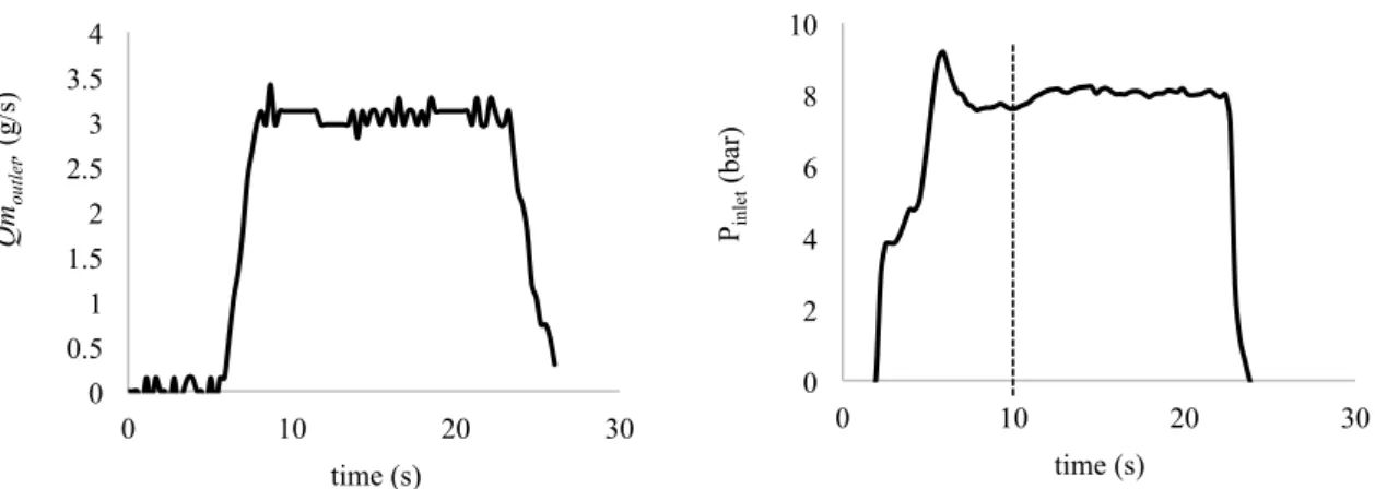
Figure 4.13 – View of the boundary layers generated on the walls (physical boundaries) of a spike in the geometric shape domain G4. ... 35 Figure 4.14 – View of the polyhedral mesh generated in Fluent for the complete geometric shape domain, G5. ... 35 Figure 4.15 – Simple schematic of the complete geometric shape domain, G5, with a zoomed in top view of a single outlet spike. ... 34 Figure 5.1 – Mass flow rate of extracted liquid coffee (outlet) and system pressure (inlet) over the time of a single extraction cycle of a Lungo capsule. ... 41 Figure 5.2 – Temperature at inlet, outlet, beaker and thermo block over the duration of the first extraction cycle of the Ristretto blend. ... 45 Figure 5.3 – Temperature at inlet, outlet, beaker and thermo block over the duration of the first extraction cycle of the Ristretto blend. ... 45 Figure 5.4 –

Plot of inlet (left) and outlet (right) temperature at the start (blue) and end

(red) of the extraction cycle versus time

. ... 45 Figure 5.5 – Transient simulation of the inlet pressure (bar) for the Mocoffee capsule system (geometry G5), over a run time of 0.3s. ... 48 Figure 5.6 - Close view of the velocity profile around one of the injection head’s spikes that perforate the flexible membrane. ... 49 Figure 5.7 – A top view of the velocity profile of shape domain of geometry 4 (injection head and flexible film). ... 49 Figure 5.8 – Velocity vector profile over a cross-sectional plane of shape domain G4. ... 49 Figure 5.9 – A vector velocity profile across the symmetrical plane of geometry 5 without headspace (steady state). ... 50 Figure 5.10 – A vector velocity profile over an axial plane of geometry 5 without headspace, one with the 19 injector spikes of the original design (first) and the other without the inner most ring of 3 injector spikes (second). The zone on the outer edge represents the fluid flow below the flexible film, while the larger inner zone represents the fluid flow above the flexible film ... 51 Figure 5.11 – A comparison of the velocity contour and vector profiles for geometry 5 with the headspace. ... 52 Figure 5.12 – Plot of the tracer concentration versus iterations at the outlet (RTD) for the base geometric shape (G5 with 19 puncture sites). For the simulation, time step size was set at 0.001 (1 iteration is the equivalent of 0.001s of simulation time, or 1s of run time for every 1000 iterations). ... 53 Figure 5.13 – Plot of the tracer concentration versus iterations at the outlet (RTD) for the altered geometric shape (G5 with only 16 puncture sites). For the simulation, time step size was

(15)

xv

set at 0.001 (1 iteration is the equivalent of 0.001s of simulation time, or 1s of run time for

every 1000 iterations). ... 53

Figure 9.1 – View 1 of injection head. ... 61

Figure 9.4 – Close view of a spike from the injector plate. ... 62

Figure 9.5 – Close view of a puncture site, with the spike from the injection head perforating the flexible film. The area between the edges of the circle and the spike is where the water flows in the simulation. ... 63

Figure 9.6 – A top view of the mesh generated for the flexible film. ... 63

Figure 9.7 – A zoomed in view of the mesh generated over one of the spikes in the filter plate at the bottom of the capsule. ... 64

Figure 9.8 – Cross-sectional cut of G5 assembly with a upwards view of the spikes on the injection head perforating the flexible film. ... 64

Figure 9.9 – Side view of the complete G5 assembly. ... 65

Figure 9.10 – Ansys Fluent workbench window for geometric shape domain G5 and variations. ... 65

Figure 9.11 –Ansys Fluent Processing window with the mesh on the right and the processing tree on the left. ... 66

Figure 9.12 – Scaled residuals monitor for a transient simulation of geometric shape domain G5. ... 66

Figure 9.13 - Scaled residuals monitor for a transient simulation of the tracer experiment for the RTD analysis of G5. ... 67

Figure 9.14 – Outline of geometric shape domain G5 (CFD Post). ... 67

Figure 9.15 – Velocity contour profile plotted over the symmetrical plane of G5 with an empty or non-porous capsule (no packed coffee bed). ... 68

Figure 9.16 – Velocity vector profile plotted over the symmetrical plane of G5 with an empty or non-porous capsule (no packed coffee bed). ... 68

Figure 9.17 – A velocity vector profile across the symmetrical plane of geometry 5 without the inner-most ring of injector spikes (16 injector spikes in total on the injector plate). ... 69

(16)

(17)

xvii

Index of tables

Table 2.1 - Mesh quality parameters, skewness and orthogonal quality (OQ). ... 16 Table 3.1 – System information of the PC used for the CFD. ... 21 Table 4.1 - Comparison table of 5 main geometries of the shape domain used in this study, from least to most complex. ... 32

(18)

(19)

xix

Nomenclature

English symbols

𝐶! Fluid specific heat J/kg K

𝐷! Diameter of the coffee particles M

g Gravitational acceleration m/𝑠!

h Enthalpy J/kg

I Turbulent intensity %

𝑘 Molecular conductivity W/m K

𝑘! Turbulent thermal conductivity W/m K

𝑙! Length of packed bed M

𝑄! Mass flow rate g/s

𝑅! Inertial resistance 1/m 𝑅! Viscous resistance 1/𝑚! S Source terms T Temperature K t Time s 𝜐 Fluid velocity m/s V Volume 𝑚!

𝑥! Cartesian coordinate in the i-direction m

𝑦 Distance to the wall m

𝑦! _{Non-dimensional wall distance}

Greek Symbols

𝛼 Permeability 𝑚!

𝜀 Porosity

𝜀!"# Bed bulk porosity

𝜇 𝜌

Molecular dynamic viscosity Fluid density

𝑚!_/𝑠 Kg/𝑚!

𝜌! Bed bulk density Kg/𝑚!

𝜌! Particle density of roasted coffee Kg/𝑚!

(20)

𝜙 Scalar quantity Dimensionless numbers Nu Pr Re Nusselt number Prandlt number Reynolds number Sub/superscripts b in out Bulk Inlet Outlet Acronyms 1-D, 2-D, 3-D CAD CAGR CFD PRESTO RAM RTD SIMPLE SIMPLEC UDF

One, two, three dimensions Computer-Aided Design

Compound Annual Growth Rate Computational Fluid Dynamics Pressure Staggering Option Random Access Memory Residence Time Distribution

Semi-Implicit Method for Pressure-Linked Equations SIMPLE-Consistent

(21)

xxi

Objectives

This work aims to build an accurate 3D model of the capsule system, Monodor, as patented by the founder of Mocoffee, and use Computational Fluid Dynamics (CFD) tools to analyse the flow of water in that same system during the extraction process. The purpose of this analysis is to achieve a better understanding of the flow behaviour throughout the capsule system and every phenomenon that occurs during the process. This understanding will make it possible to determine the impact of the design of the main extraction components on the flow and how, or to what extent, it can be simplified without compromising the efficiency of the extraction.

Similar to other CFD analysis works, the simulation will be performed following a three-step process. These steps are: pre-processing, processing and post-processing.

Pre-processing, the first step, encompasses all of the tasks performed before the actual numerical solution process, which includes a careful evaluation of the flow problem being presented and how the solution should be approached, meshing the problem domain and generating the computational model.

For this step, the shape of the problem domain, which is represented by the main components of the Mocoffee coffee extraction system, will be created in Solidworks, a 3D CAD and CAE design software, developed by Dassault Systèmes. During this process, a number of variations on this shape will be created, from a very simplified version of the fluid flow, to a version that better represents the complexity of the extraction system, as well as a few alterations to the design in order to then study its impact on the flow. Each will be exported to Ansys Mesh software, where the domain will be meshed and the computational model generated.

Processing is the second step, where the CFD software, in this case Ansys Fluent, will take all of the determined model input values and solve the mathematical equations of the established water flow until it achieves a required accuracy or acceptable convergence.

Post-Processing is the third and final step, where the results obtained in the Processing step can be evaluated, both numerically and graphically. The data generated by Fluent for all the different models will be analysed in CFD-Post, not just in terms of important output values like mass flow, but also through means of graphs, contour plots and vector plots of velocity and pressure fields to better compare these models and evaluate the impact they have on the water flow.

(22)

xxii

To validate these models, experimental data will be acquired through the performance of various extractions with different coffee blends, using the same capsule extraction system that is currently used by Mocoffe.

(23)

1 1. Introduction

1.1. CFD as an analysis tool

Computational Fluid Dynamics (CFD) is a branch of fluid mechanics which uses applied mathematics to model fluid flow in any given system to predict momentum, heat and mass transfer mechanics, being therefore nowadays an indispensable tool that might help to determine the optimal design of any industrial process or equipment’s. The success of a good CFD analysis lies in how the simulation numerical results can match the experimental data or how well it can predict complex phenomena that cannot be isolated in the laboratory.

As a tool, a well-designed CFD analysis will allow a deeper and better understanding of what is happening in any given system or process, particularly where detailed measurements of certain variables (ex. high temperatures or high pressures) and phenomenon are rather impossible or incredibly difficult to undertake. It also makes it possible to evaluate the impact of geometric variations and other changes to the system in a shorter time frame and with lower costs than in a typical laboratory testing (Bin Xia, 2002).

Only recently the food industry has been applying simulation tools like CFD. It has increasingly been used to analyse flow and the performance of process equipment, such as spray dryers, baking ovens, stirred tanks, heat exchangers and refrigerated display cabinets (Xia & Sun, 2002) mainly due to the exponential rise of the processing power of computers over the last years, as well as the increasing availability of powerful yet user friendly software.

As recently as 2013, there have been articles about modelling and validating heat and mass transfer in various stages of the coffee making process using CFD analysis, including earlier stages, such as the coffee roasting process (Alfonso-Torres & Hernández-Pérez, 2013) or even the coffee packaging in capsules (Spanu, Mosna, & Vignali, 2016). As an example of the real industrial applications of these CFD studies, in 2014, Petroncini, an Italian developer of coffee roasting equipment, used CFD models to simulate the roasting of coffee beans in one of their industrial roasters to improve both quality control and the heat transfer rates (Wasserman, 2014).

(24)

2

1.2. Single-serve coffee container

Coffee is one the most consumed beverages worldwide. The International Coffee Organization reported that, from 2015 to 2016, consumption of coffee, which is measured in 60 kg bags of coffee, was about 155 million bags worldwide (International Coffee Organization, 2017). It is part of an enormous industry, with the OEC (the Observatory of Economic Complexity) estimating that coffee was in the top 100 most traded products worldwide and worth $30 billion in exports just in the year 2015. The top exporter of coffee remains Brazil and the top importer the USA, at $5.87 billion and $5.65 billion, respectively (OEC, 2015).

Coffee beverages are prepared from the green coffee beans through a process that involves roasting and grinding the raw coffee beans, and then mixing them with hot water, allowing it to brew. The brewing process can be done slowly, by drip or filter, for example, or very quickly and under pressure by using espresso machines.

An espresso coffee is brewed by forcing hot water to pass through a bed of densely compacted and finely ground coffee at a pressure of about 9 bar (Caballero, Finglas, & Toldra, 2015). The quality of a small, aromatic cup of espresso depends, not only on the quality of the coffee beans and extraction water, but also, to a larger extent, on an integrated brewing system that consists of a brewing machine, a grinder and other accessories.

The housing of a typical brewing espresso machine conceals a water reservoir, a pump to force the brewing water through the coffee, and a boiler in which the water is held and heated. The apparatuses that heat water for brewing and make steam for milk frothing are separate, since the ideal water temperature for brewing, about 90ºC, is slightly lower than the one required for producing steam. (Davids, 2013)

Eric Frave, a Nestlé employee, first invented and patented the Nespresso capsule system, the first single-serve coffee container system, in 1976. This is a method for brewing and serving espresso coffee for a single portion, which is accomplished by pre-packaging individual portions of grinded coffee beans, either in coffee pods, capsules or bags.

Though it may have started as a niche market, the coffee capsule industry has developed into a complex value chain over the years. According to a report published by Technavio, the market is anticipated to grow at a steady rate with a CAGR (Compound Annual Growth Rate) of close to 10% during the forecast period (2017-2021), with their growing popularity among consumers being pointed to their one-time use and disposable features (Technavio, 2017).

(25)

3

The single-serve coffee capsule system has democratised the espresso beverage by making it accessible to the domestic consumer, and it certainly has many advantages, including the simplification of preparation and the quality consistency of the brewing process. It also makes it possible to keep the unused product fresher for longer periods of time without it going stale whenever the multiunit package is opened. In addition, it affords the consumer a wide range of different coffee blends to choose from, each of these suitable for different periods of the day. Nevertheless, its main problem continues to be its environmental impact. Aluminium and plastic, the materials mostly used for the system, are damaging for the environment if not recycled properly.

In 1991, Eric Favre, after leaving Nespresso, invented and patented a new simplified capsule system, which does not use aluminium and is referred to as Monodor system. This system was firstly licensed to Lavazza worldwide and to Migros (DELICA) in Switzerland.

In order to keep the extraction process sustainable for food contact, the Monodor system has replaced the aluminium capsule for a thermoformed capsule made entirely of polypropylene, a polymer with high boiling point that is often used in food packaging for its safety and ease to recycle. This material is highly incinerable, which means that the capsules, even if not properly recycled, can be burned alongside household waste without significant damage to the environment (MoCoffee).

Later, in 2010, Favre founded the company Mocoffee A.G., as a spin off from the Monodor SA, with products that are sold internationally, including their close patented system of coffee capsules and their very own patented coffee espresso machine, called the Bossa, which use the Monodor system. Since February 2015, Mocoffee is co-owned by two Brazilian groups, wine.com.br and Tristao Group, the former is one of the biggest green coffee traders worldwide, with more than 80 years of history in the coffee industry.

Currently, Mocoffee Europe is a vertically integrated coffee company that brings the culture of the Brazilian coffee and the Swiss technology heritage to the world, being now settled in Portugal. The business structure is split in two different commercial structures:

i) The MOcoffee branch, which commercializes its own brand, enabling the exploitation of the high-quality coffee experiences business, levering the Brazilian origin.

(26)

4

ii) The Made with MO or OEM (Original Equipment manufacturer) Business that commercializes the MOcoffee platform to third parties through a private label model, enabling others to develop a high quality coffee business.

The MOcoffee brand is particularly focused on the Latin American market and USA, while the Made with MO is being commercialized in Europe, Asia and Oceania.

1.3. Monodor capsule system

The CFD analysis will be performed on the patented single-serve coffee container system invented by Eric Favre and Jacques Hentsch, referred to as Monodor. A more detailed description of the patent can be found under the publication number US8875617 B2 (Frave & Hentsch, 2011).

Figure 1.1 – A cross-sectional view of a part of the

device for preparing a beverage, showing a portion of an injection head and of a capsule carrier in which is nested a capsule, both in their initial positions.

Figure 1.2 – A detailed partial view illustrating the

penetration by the perforating spikes of the injection head into a flexible membrane of the capsule, in a more advanced phase of the water injection.

The Monodor system comprises a device for preparing a beverage from a capsule containing a product with a substance to be extracted, in this case coffee, by the injection of hot water into said capsule.

This device includes:

(a) An injection head (3) comprising a perforating surface (24) with a shape that is substantially curved and convex, provided with 19 perforating spikes (25) distributed

(27)

5

over its surface, each one with a smooth tapered shape without sharp edges and an average cone angle less than 60º, and one channel (23) arranged to supply water onto the perforating surface.

(b) A capsule carrier (4) comprising a sidewall (5), a bottom wall, an intermediate bottom wall (6) in the form of a filtering wall with 18 perforating spikes (9) and outflow orifices (10).

(c) A lower cavity portion arranged between the filtering wall and the bottom wall (12), wherein the bottom wall comprises and outflow channel (13) surrounded by a lip (14) that protrudes upwards with respect to the lowest point (15) of the lower cavity portion (7).

(d) A capsule (1), which comprises a shell that is substantially rigid, the shell further comprising a sidewall (8) and a bottom wall (11) to form the container in which the beverage (2) is contained. There is also an annular flange section (18) extending substantially in a radial plane R, whereby the flexible membrane (17) is bonded or welded. The flexible membrane is made from a multiple layer sheet, and both this membrane and the shell are made of polypropylene.

During the extraction process, the injection head perforates various smooth holes, distributed over the flexible membrane, urging this same membrane against the coffee inside or applying a tensile force to the membrane. This makes it so the water, injected onto the membrane through the supply channel on the injection head, deforms the membrane in the direction of the coffee inside the capsule and penetrates into the capsule via the smooth holes without causing them to tear.

The described method is believed to ensure a good distribution of the injected water in the capsule and makes it possible to retain a counter pressure within the capsule, to optimise the coffee extraction.

In the case of products that leave behind spent material in the capsule, as is the case with ground coffee, the pressure exerted by the upper membrane of the capsule against the coffee makes it possible, on one hand, to avoid the formation of preferential flow channels and, on the other hand to retain a counter pressure to the injection pressure, so as to ensure that the extraction proceeds during the entire extraction cycle at a high pressure. This optimises the extraction,

(28)

6

ensuring a more thorough extraction of the coffee contained in the capsule and making it possible to achieve a richer flavour and obtain a very good froth.

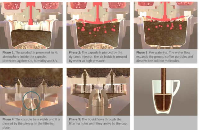
The illustration bellow (figure 3) briefly describes the different phases of the dynamic espresso brewing process of the Monodor system.

Figure 1.3 – Illustration and description of the different phases of the espresso brewing process of the Monodor

capsule system.

From the observation and analysis of the 5 phases of the Monodor brewing system, one can see that it constantly changes over time, making it extremely dynamic. Unlike other capsule systems, where the coffee is highly compacted in a non-variable capsule volume, this capsule has a headspace composed of nitrogen (to increase shelf life) and coffee volatiles in which coffee moves freely. Furthermore, at a given pressure the concave bottom of the capsule collapses, increasing the total volume of the system which, when coupled with the additional headspace, promotes a natural expansion of the coffee cake inside once it contacts with the hot water, thus creating a very short pre-infusion.

Due to their dynamic nature, phases 1 to 3 are the most complex and resource-intensive in regards to computational analysis. Due to time constraints and for the sake of simplicity, this study will concern itself mainly with phases 4 to 5 of the extraction process, meaning that the

(29)

7

simulation will start by assuming that the capsule has already been pierced by both the injection head and the filtering plate.

(30)

(31)

9 2. Mathematical Modelling

ANSYS Fluent, and other CFD software packages, simulate all flows by solving a set of mathematical equations for a finite domain.

The governing equations, which describe how unknown variables change over time, apply to most fluid flow situations and include the following conservation laws of physics:

• Conservation of mass

• Conservation of momentum, from Newton’s second law • Conservation or energy, or the first law of thermodynamics

Fluent works by solving these governing integral equations for the appropriate scalars, using a control-volume-based technique (in the case of 3-D analysis) that consists of:

a) Dividing the domain into discrete control volumes using a computational grid (the mesh)

b) Integrating the governing equations on the individual control volumes to construct algebraic equations for the discrete dependent variables such as velocities, pressure and temperature

c) Linearizing the discretized equations and solution of the resultant linear equation system to yield updated values of the dependent variables.

A more detailed description of all these governing equations from which the equations solved by Fluent are derived, plus their solved forms, can be found in ANSYS Fluent 12.0 Theory Guide, and User’s Guide.

2.1. Conservation of mass

For the CFD analysis of the problem in study, the Eulerian description of fluid motion was considered. This means that fluid properties change at a fluid element (the control volume) that is fixed in space and fluid can freely pass through the volume’s boundary.

Applying the model of a finite control volume fixed in space, a statement of the conservation for mass can be obtained in the form of a partial differential equation, in conservation form:

(32)

10

!"

!"+ ∇ ∙ 𝜌𝜐 = 𝑆! [2.1] Where 𝜌 is the density and 𝜐 the velocity vector of the fluid. The first term on the left side of the equation, !"_!", describes the change in density, the second one on the left, ∇ ∙ 𝜌𝜐 , is the convective term, which describes the net flow of mass across boundaries, and 𝑆! is the mass source. Since no mass is produced or added to the coffee capsule extraction system, then 𝑆! = 0.

!"

!"+ ∇ ∙ 𝜌𝜐 = 0 [2.2] This equation is often referred to as the continuity equation.

If an incompressible flow is considered for the system, !"

!"= 0, then the equation will be reduced to:

∇ ∙ 𝜌𝜐 = 0 [2.3]

2.2. Conservation of momentum

The conservation of momentum is represented by the Navier-Stokes equations, which are the basic governing equations for a viscous, heat conducting fluid.

Taking from these equations, the conservation of momentum in an inertial reference frame can be described by:

!

!" 𝜌𝜐 + ∇ ∙ 𝜌𝜐𝜐 = −∇𝑝 + ∇ ∙ 𝜏 + ρ𝑔 + 𝐹 [2.4] Where 𝑝 is the static pressure, 𝜏 (described below) is the stress tensor for a fluid, and 𝜌𝑔 is a term that describes the gravitational body force, with 𝑔 being the gravitational acceleration. The term 𝐹 contains other source terms that may arise from external body forces, or other model-dependent source terms such as porous-media and user-defined sources.

(33)

11

𝜏 = 𝜇 ∇𝜐 + ∇𝜐! ₋!

!∇ ∙ 𝜐𝐼 [2.5] Where 𝜇 is the molecular viscosity, 𝐼 is the unit tensor, and the second term on the right hand side of the equation (−!_!∇ ∙ 𝜐𝐼) is the effect of the volume dilation.

2.3. Energy conservation

The energy equation for a fluid region is written in terms of sensible enthalpy, ℎ, defined as: ℎ = _!! 𝐶_!𝑑𝑇

!"# [2.6]

Where 𝑇 is temperature, 𝑇_!"# is the reference temperature and 𝐶_! is the specific heat. The energy equation will then be as follows:

!

!" 𝜌ℎ + ∇ ∙ 𝜌ℎ𝜐 = ∇ ∙ 𝑘 + 𝑘! ∇𝑇 + 𝑆! [2.7] Where 𝑆! is a source term that includes any volumetric heat sources that have been defined, 𝑘 as the molecular conductivity, and 𝑘! as the conductivity due to turbulent transport.

2.4. Porous media

Most of the flow throughout the system occurs inside the capsule, which will be filled with finely ground and compacted coffee. The flow of water through the solid coffee inside the capsule can be modelled as a fluid flow through a packed bed, so it is important to understand the equations used to define a porous media. The Ergun equation is applicable over a wide range of Reynolds numbers and for many types of packing:

∆! ! = !"#! !!! (!!!)! !! 𝜐!+ !.!"! !! (!!!) !! 𝜐!! [2.8] Where 𝜀 is the porosity and 𝐿 the length of the bed, and 𝐷! is the diameter of the bed particles. In the case of laminar flow in the porous region, the second term in the Ergun equation may be dropped, resulting in the Blake-Kozeny equation:

∆! ! = !"#! !!! (!!!)! !! 𝜐! [2.9]

(34)

12

For transient porous media calculations, the effect of porosity on the time-derivate terms is accounted for in all scalar transport equations and the continuity equation, with the time-derivate term itself being now defined as follows:

!

!"(𝜀𝜌𝜙) [2.10] With 𝜙 defined as a scalar quantity.

The bulk porosity of the packed coffee bed can be calculated using the following relation:

𝜀!"# = 1 −!_!!

! [2.11]

Where 𝜌! is the bed bulk density, 𝜌! is the particle density of the roasted coffee and 𝜀!"# is the bed bulk porosity. The packed bed is assumed isotropic, meaning that the porosity and permeability of the bed are uniform across all directions.

Permeability is a key parameter affecting extraction, as it determines the flow rate through the bed and, consequently, the brewing time. This, in turn, affects the mass transfer from bed to cup, impacting brewing quality. It can be calculated using the following relation:

𝛼 = !!!!!

!"#(!!!)! [2.12]

Where 𝛼 is the permeability of the porous media. In turn, the inverse of this permeability is the resistance of the porous media to the fluid flow. The viscous, 𝑅!, and inertial, 𝑅!, resistances can be determined from the Ergun and Blake-Kozeny equations:

𝑅_!=!"# (!!!)!

!!_!_!!_!! [2.13]

𝑅!=!.! (!!!)_{! !}

! !! [2.14]

In which 𝐷! is the diameter and 𝜑 is the sphericity of the particles that make up the medium. The main objective of this study was to build the physical model of the capsule coffee system and simulate the fluid flow through both the non-porous and porous parts of the system.

(35)

13

Consequently, and due to the limited time, this work did not cover the kinetics of coffee extraction, and thus the transport of coffee solubles was not modelled.

2.5. Modeling turbulence

The fluctuation of velocity fields in turbulent flows result in the mixing of transported quantities such as momentum, energy and species concentration, while also causing the fluctuation of transported quantities. These fluctuations can be of a very small scale, which makes them too computationally expensive to simulate directly.

This problem is solved by time averaging or otherwise manipulating the governing equations to remove these small scales. The result is a modified set of equations that can be much more easily, and less expensively, solved. Turbulence models are needed to determine the value of the additional unknown variables contained in these equations.

There are three approaches in terms of computational models of turbulent flows:

a) Reynolds-Averaged Navier-Stokes (RANS) models, an approach in which ensemble-averaged (or time-ensemble-averaged) Navier-Stokes equations are solved and where all turbulent length scales are modeled.

b) Large Eddy Simulation (LES), which solves the spatially averaged Navier-Stokes equations, with large eddies being directly resolved, but eddies smaller than the mesh being modeled.

c) Direct Numerical Simulation (DNS), which resolves the whole spectrum of scales without any modeling being required.

2.5.1. Reynolds-Averaged Navier-Stokes (RANS) model

The RANS model has been the most widely used approach for calculating industrial flows, mainly due to how greatly it reduces the computational expenses and effort compared to other approaches.

In Reynolds averaging, the solution variables in the instantaneous Navier-Stokes equations are decomposed into the mean and fluctuating components.

(36)

14

For the velocity components:

𝜐! = 𝜐!+ 𝜐!! [2.15] Where 𝜐! and 𝜐!! are the mean and fluctuating velocity components (𝑖 = 1,2,3).

Likewise, for pressure and other scalar quantities:

𝜙 = 𝜙 + 𝜙!_[2.16] Where 𝜙 denotes a scalar such as pressure, energy, or species concentration.

Substituting expressions of this form for the flow variables into the instantaneous continuity and momentum equations and taking a time (or ensemble) average yields the ensemble-averaged momentum equations. They can be written in Cartesian tensor form as:

!" !"+ ! !!! 𝜌𝜐! = 0 [2.17] ! ! 𝜌𝜐! + ! !!! 𝜌𝜐!𝜐! = − !" !!!+ ! !!! 𝜇 !!! !!!+ !!! !!!− ! !𝛿!" !!! !!! + ! !!! −𝜌𝜐! !_𝜐 !! [2.18]

These are called the Reynolds-averaged Navier-Stokes (RANS) equations, which have the same general form as the instantaneous counterparts, but with the velocities and other solution variables now representing ensemble-averaged (or time-averaged) values.

The additional terms that appear in these equations, such as the Reynolds stresses, −𝜌𝜐_!!_𝜐 !!, represent the effects of turbulence, and as such, must be modeled in order to close the equations.

2.6. Discretization of governing equations

To obtain the values of the dependent variables at different times and positions, the aforementioned system of governing partial differential equations (PDE’s) need to be resolved. However, in most situations, these equations cannot be solved analytically. Discretization methods are implemented in CFD to convert the partial differential equations into algebraic equations (also called discretised equations), which can then be solved numerically by reliable and robust algorithms.

(37)

15

These discretization methods can be broadly classified in mesh (or grid) based methods and mesh-free methods. CFD software programs commonly use mesh-based methods, which can be further classified into finite-difference and finite-volume discretization.

2.6.1. Finite-volume method (FVM)

The finite volume method is the most widely applied method in CFD, and the one implemented in the FLUENT software, due to its simplicity and ease of implementation for both structured and unstructured grids. This is a technique where the governing equations are integrated over a finite control volume (CV) to obtain the discretized equations.

The first step in this method is to divide the domain into a number of discrete control volumes, with the variable of interest located in the centroid of the control volume. This is achieved through the process of grid generation, or meshing.

Meshing involves dividing the domain shape into numerous cells of many shapes and sizes, referred to as elements and volumes, which are all connected by nodes. In 2D domains, these elements can take the shape of quadrilaterals or triangles. In the case of 3D domains, these can take the shape of a tetrahedral (four sides), prims and pyramids (five sides) or hexahedral (six sides).

(38)

16

Quadrilateral and hexahedral elements (2D and 3D, respectively) make up structured grids, which typically lower the computational requirements and improve the speed of the numerical simulations. On the other hands, triangles and tetrahedral elements (2D and 3D, respectively) are typically used in unstructured grids, which fill the domain with an arbitrary collection of elements or cells.

A well-defined domain shape may require a denser mesh, which means a greater number of smaller elements that can capture the most important characteristics of the flow. On the other hand, a greater number of elements in a mesh increases processing requirements, making the whole process time consuming, so a compromise between these two aspects must be achieved.

When it comes to meshing quality, fluent checks for two parameters: the minimum orthogonal quality, maximum orthogonal skew and maximum aspect ratio.

Skew is defined as the difference between the shape of the cell and the shape of an equilateral cell of equivalent volume. Highly skewed cells can decrease accuracy and destabilize the solution. As a general rule, the maximum skew for a triangular/tetrahedral mesh in most flows should be kept bellow 0.95. (ANSYS, Inc., 2013)

Orthogonal quality in Ansys Fluent is equivalent to orthogonal skew, except that the scale is reversed. However, these values may not necessarily correspond to one another, as the computation depends on boundary conditions on internal surfaces. Orthogonal quality values should be kept above 0.1. (ANSYS, Inc., 2013)

Table 2.1 - Mesh quality parameters, skewness and orthogonal quality (OQ).

Mesh Quality Parameters

Inacceptable Bad Acceptable Good Very Good Excellent

Skewness 0.98-1.00 0.95-0.97 0.80-0.94 0.50-0.80 0.25-0.50 0.00-0.25

OQ 0-0.001 0.001-0.1 0.10-0.20 0.20-0.69 0.70-0.95 0.95-1.00

Aspect ratio is defined as a measure of the stretching of a cell, computed as the ratio of the maximum and minimum value of the distances between certain centroids and nodes in the element. (ANSYS, Inc., 2013)

Ansys Fluent also provides the ability to improve smoothness by refining the mesh based on the change in cell volume or the gradient of cell volume. This smoothens out the rapid changes in

(39)

17

cell volume that can occur between adjacent cells and result in larger truncation errors. (ANSYS, Inc., 2013)

(40)

(41)

19 3. Materials and Methods

3.1. Equipment

3.1.1. Extraction Installation

To measure variables such as temperature, pressure and flow rate at various points of the extraction process, an installation was mounted in the laboratory.

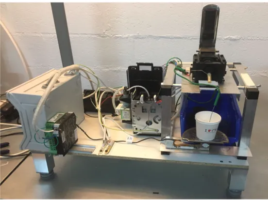
This custom-made structure (JIG) consisted of a fixture built around an extraction chamber, which was removed from an original Mocoffee espresso machine, plus a separate boiler, a pump and other components necessary to replicate the extraction process of the original machine. In addition, a number of sensors were strategically placed at various points of the described structure, in order to measure the extraction variables, like temperature and mass flow, throughout the extraction process.

Figure 3.1 - The custom-made structure (JIG) used for the experiments and data recollection.

The machine has the following components:

• Extraction chamber • Filter

(42)

20

• Boiler

• Pump (Ulka pump EP4)

• Thermocouples (type k, with a response time of 0.8s, one at the inlet, one at the outlet, one inside the beaker and one in the boiler)

• Pressure sensor (transducer 0-25bar, response time of 5ms) • Weight cell (0-0.3kg)

A basic diagram of the extraction process for the JIG can be seen below in figure 6.

Figure 3.2 - PID of the custom-made extraction machine (JIG). Temperature sensors are identified as 1 (inlet),

TI-2 (outlet) and TI-3 (beaker), and pressure sensor as PI-1 (inlet).

The data measured by the sensors was collected and processed by a data acquisition system (DATAQ Instruments), consisting of the physical components of the data logger and the respective software. Water tank Boiler Pump Flow meter Drip tray

(43)

21

Figure 3.3 - An 8-Channel USB Data Logger and Data Acquisition System for DI-8B Amplifiers Model DI-718-US,

and a DATAQ Instruments Resource CD (December 2015) used to install the WinDaq Software.

The input analogy amplifiers channels for data acquisition came already calibrated from factory. The data input for the different sensors was checked through the following methods:

• Thermocouples: immersion on an ice-cold bath and boiling water; • Cell weight: using known precision weights:

• Pressure: comparison with a calibrated analogic pressure gauge.

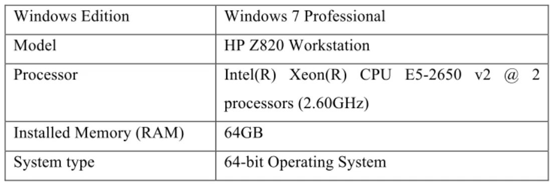
3.1.2. Computer Information

The PC used for the CFD analysis had the following system information:

Table 3.1 – System information of the PC used for the CFD.

Windows Edition Windows 7 Professional

Model HP Z820 Workstation

Processor Intel(R) Xeon(R) CPU E5-2650 v2 @ 2

processors (2.60GHz)

Installed Memory (RAM) 64GB

(44)

22

3.2. Materials

The materials used in the extraction experiments can all be found in laboratory 427 of the Chemistry Department and are as follows:

• 4 distinct types of coffee capsules from the Mocoffee brand Crème, Espresso, Lungo (400𝜇𝑚) and Ristretto (300𝜇𝑚) in capsule format (6.5 ± 0.2g of coffee grounds in each capsule);

• Costa Rica Bella Vista blend from Fioresso coffee capsules (6.5 ± 0.2g of coffee grounds in each capsule);

• Transparent polypropylene capsules; • Polypropylene capsule films;

• Beaker (200ml) • Laboratory spatula

Mocoffee provided all the coffee capsules, both the transparent and commercial ones with the different coffee blends, as well as the polypropylene film and the equipment needed to seal the capsules. The laboratory provided the rest.

3.3. Experimental Methods

A number of coffee extractions were performed, using the aforementioned equipment, in order to obtain experimental data that could be used to validate the results obtained in the CFD analysis of the system.

The experimental data was collected from the pressure, temperature and weight sensors that were installed in the device.

3.3.1. Fluid flow analysis

In order to analyse the flow of water through the extraction chamber, 5 extractions were performed for each of the 4 espresso coffee blends listed in the materials section: Crème, Espresso, Lungo and Ristretto, making for a total of 20 extractions done in succession.

The machine was calibrated so that it would extract the same amount of coffee from each capsule, 50ml of liquid coffee into the beaker, with an average extraction time of 25s.

(45)

23

3.3.2. Thermal analysis

For the thermal analysis of the system, a sample size of 20 capsules of the Ristretto espresso blend was used. The machine was also calibrated to extract 50 ml of liquid coffee into the beaker, resulting in an average extraction time of 25s.

At the start of the experiment, the components of the extraction chamber are at room temperature and gradually heat up with every extraction, up to a point where the heat losses in the extraction domain are negligible. These consecutive extraction cycles were performed in order to study how this gradual heating affects the temperatures at the inlet, outlet and beaker during the process.

(46)

(47)

25 4. Computational Models and Methods

4.1. Pre-Processing

4.1.1. Geometry and shape of domain creation

The 3D models of the main parts that make up the extraction process system were built using the 3D CAD design software, Solidworks 2016. They consisted of the following: the injector head, the coffee capsule, the film that seals the capsule and the bottom filtering wall that punctures the bottom of the capsule.

Figure 4.1– Model of the injection head built in Solidworks (left) and the real life component found inside the device

(right).

The coffee capsule, and the flexible membrane that is welded over its annular flange section, were built separately in Solidworks. This choice was made in order to facilitate further adjustments to the film, like the size of the perforated holes and the curvature of the film itself, which are necessary to better simulate the deformation of the membrane during the injection and extraction phases.

(48)

26

Figure 4.2 – Model of the coffee capsule (left) and flexible membrane (right) built in Solidworks.

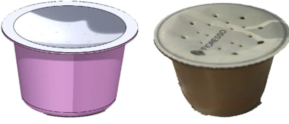
Figure 4.3 – Model of the coffee capsule and flexible membrane assembled in Solidworks (left) and the real life

commercial version (right).

Figure 4.4 – Model of the perforating bottom wall built in Solidworks (left) and the real life component found inside

(49)

27

These separate parts were all assembled in Solidworks to form the complete model of the extraction design.

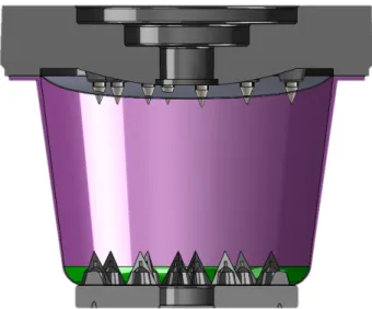
Figure 4.5 – A cross-sectional viewof the four different components of the Monodor extraction system assembled in

Solidworks.

In order to conduct the CFD analysis, however, it was necessary to create a shape domain, which would correspond to the space between the confines of the design where the water would flow.

This was accomplished by using basic tools available in Solidworks, which allowed the entire model to be “filled”, similar to a mould, and the enveloping structure to be removed, thus obtaining a shape domain that would function as the fluid system.

This process was repeated throughout the models used and analysed in this work, starting from the most basic and increasing the complexity of the design until a model that could successfully simulate the real extraction process was obtained. By order of complexity, these models, or physical geometries, were as follows:

Geometry 1, or G1, consisted of the coffee capsule and the top film parts. A simplified version

of the actual system’s inlet and outlet were used. The inlet in this first model consisted of 19 holes on the top film, each 1.4mm in diameter, that simulate the puncture sites created by the injector part, and the outlet consisted of similar holes, 5 in total, on the bottom part of the capsule that served as an outlet for the fluid.

(50)

28

Figure 4.6 - Different views of Geometry 1.

Geometry 2, or G2, consisted of all the parts, except the injector head, meaning the top film,

the capsule and the bottom filter. This model had the same inlet as G1, but the 18 holes of the bottom filter were selected as the outlet. G2 served to analyse the water flow through the porous bed and to optimize the mesh in this highly complex area.

(51)

29

Figure 4.7 - Different views of Geometry 2.

Geometry 3, or G3, consisted of a model similar to G2 in almost all aspects, with the only

difference being that the size of the holes on the top film was adjusted in order to better fit the reality of the design. The diameter of the outer circle of holes was kept at 1.4 mm, while the diameter of the inner circle of holes was reduced to half, 0.7mm, in order to take into account the curvature of the injector, the height of the peaks and the curvature of the film as water pushes it inward.

(52)

30

Figure 4.8 – Different views of Geometry 3.

Geometry 4, or G4 consisted of the injector and the top film. This model had the injector water

inlet as the system inlet, 6.2mm in diameter, and the 19 holes in the top film as the system outlet. G4 served to analyse the flow of water before it enters the capsule and passes through the porous bed, as well as to optimize the mesh in this area.

Figure 4.9 – A full view and cross-sectional cut of Geometry 4.

Geometry 5, or G5, consisted of all the parts of the system, meaning the injector, top film,

capsule and bottom filter. This model had the water channel of the injector as the system inlet, and the holes in the bottom filter as the outlet. This model served to analyse the flow of water in both non-porous (injector) and porous zones (capsule) of the system.

(53)

31

Figure 4.10 – Different views of Geometry 5.

Though each of these geometries were subject to alterations and improvements, the final geometry, G5, had three sub-geometries, or variations, created with the goal of studying their effect on the fluid flow model.

Some of these variations were done in Solidworks, like a) increasing the curvature of the film to better replicate the perforation by the injection head and b) decreasing the number of spikes of the injection head and, consequently, the number of punctures on the film. Other variations involved changes to the Fluent model, like c) creating a headspace inside the capsule and d) creating distinct zones on the porous bed with different porosities. However, the components, inlet and outlet of all these G5 variations remained unaltered.

Tackling the geometry and mesh optimization step-by-step made it possible to speed up the overall computation process. Simulating particular components of the geometry separately, especially in the more complex zones, spared the work a lot of computing power and solution convergence time that using the complete geometry unoptimized from the very beginning would entail. Thus, with a well-defined geometry and mesh for the more complex zones, it was easier to obtain a converged solution in the final complete geometry.

The key differences between each of the five main geometries are highlighted in the following comparison table.

(54)

32

Table 4.1 - Comparison table of 5 main geometries of the shape domain used in this study, from least to most

complex.

Geometry Components/Parts Inlet Outlet Image

G1 Capsule; top film

19 puncture sites (1.4 mm in

diameter) through the top

film

5 holes through the bottom of the

capsule

G2

Capsule; top film; spikes from bottom

filter G1 inlet 54 holes = 18 spikes from bottom filter × 3 holes on each spike G3

Capsule; top film; spikes from bottom

filter

G1 inlet (two most inner rings

are 0.7 mm in diameter)

G2 outlet

G4 Injector head; top

film Water channel (6.2 mm in diameter) G3 inlet, minus space occupied by spikes G5

All parts (capsule; top film; spikes from

bottom filter; injector head)

G4 inlet G2 outlet

Some components of the overall shape domain were simplified during the step-by-step process to improve the overall meshing of the complete body, granted that simplification did not impact the flow in any significant way. Both the physical geometry and the expected flow pattern in each model had mirror symmetry, so the models were cut along that plane, and symmetry boundary conditions were later applied to the resulting new surfaces. These alterations were done with the tools provided by both the Solidworks and Fluent software, with the explicit goal of lowering the processing time and requirements of each simulation.

(55)

33

4.1.2. Mesh Generation

The next step in the Pre-processing stage is the generation of a grid, or meshing. Due to the complexity of certain elements in the geometric domain of the capsule system, more specifically the puncture sites, a structured hexahedral mesh could not be obtained for the whole domain. Instead, an unstructured mesh made up of tetrahedral cells was used for the entire geometry.

Some care was taken to make sure that the grid was flow-aligned, thus minimizing numerical dispersion and increasing the accuracy of the simulation, and to maintain a similar topology across the surfaces of any given geometric volume. Figure 16 illustrates the sort of mesh applied in the geometric domain.

Figure 4.11 – Different views of the unstructured grid generated for geometric domain G4 (injection head and

(56)

34

To capture velocity and temperature gradient information at the fluid-surface boundaries, it becomes important to model the boundary layer. The key to a fairly accurate solution for the fluid flow problem lies in properly meshing the fluid domain at the boundary layer, in order to fully capture its effects on the flow.

Generally, this involves accommodating a higher number of cells, which are stacked one over the other in the direction normal to the fluid flow. This approach ensures meshing elements of higher quality without necessarily increasing the number of grid cells and computation time.

ANSYS Fluent offers a feature called inflation, which was used to create these stacked elements in the direction normal to the boundary. The way it achieves this is by basically inflating the mesh with several layers from the surface of the boundary, until it fully covers the boundary thickness layer.

These inflation layers were introduced in the domain to capture the boundary layers at the various solid walls that make up the physical boundaries of the geometry. These layers had at least 5 grid points in the direction normal to the respective wall, with a total thickness that corresponded to a value of 𝑦!_{(dimensionless wall distance) that should sit within the accepted} values of the chosen turbulent model.

(57)

35

Figure 4.13 – View of the boundary layers generated on the walls (physical boundaries) of a spike in the geometric

shape domain G4.

The Fluent solver is face-based, and thus supports meshes composed of polyhedral cells, which have the benefit of a lower overall cell count, 3-5 times lower in the case of unstructured meshes, when compared to those with tetrahedral or hybrid cells.

Figure 4.14 – View of the polyhedral mesh generated in Fluent for the complete geometric shape domain, G5.

In the setup portion of Fluent, a smoothing option is available to improve the quality of the mesh by “correcting” a portion of the mesh elements with higher skew. These meshing conditions produced a mesh quality with a maximum skew lower than the 0.95 and orthogonal quality higher than the recommended 0.01. The number of mesh elements was kept below 2×10!!"_{to avoid making the simulations resource-intensive and lowering simulation time,} while also keeping it high enough so as to not significantly lower the accuracy of the prediction.

(58)

36

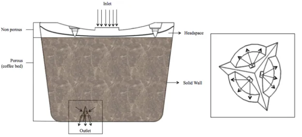
4.1.3. Selection of physical boundaries

The physical boundaries were set in the same Meshing mode that was used to create the grid, a tool provided by the CFD solver software, Fluent. Figure 17 illustrates a basic schematic of the physical boundaries of the complete and final geometry (G5).

After generating the mesh and defining these boundaries, Fluent then imports the mesh to a solver. There, the fluid properties, turbulent quantities and boundary conditions need to be provided (or “setup”) in order for Fluent to then use the finite volume method to solve the transport equations and find a reliable and accurate solution to the fluid problem.

4.2. Processing

4.2.1. Setup

When doing fluid flow calculations, water is often considered incompressible. Given this and the fact that the speeds observed during the extraction process are not particularly high (Mach number well below 0.3), the pressure-based type solver was chosen as the most appropriated for this sort of flow. This solver assumes that pressure in the system is not a function of temperature and density, so the pressure field is determined by solving a pressure equation (obtained by manipulating the continuity and momentum equations).

The absolute velocity formulation was enabled, as it is preferred in situations where the flow in most of the domain is not rotating, which is the case with the extraction process. The effects of gravity on the flow, however, were considered, with its value set at 9.8 m/s2_{. The direction of}

Figure 4.15 - Simple schematic of the complete geometric shape domain, G5, with a zoomed in top view of a single

(59)

37

the gravitational acceleration was set in the positive x-vector direction, because, and although the geometry of the capsule and its components was built in an upright position, in reality, it is laid sideways in the extraction chamber for the Bossa Machine. In the case of other Mocoffee coffee machines, the system is held in vertical position.

A viscous model was chosen in order to specify how the fluid flow would be calculated. Apart from some special cases, the k-𝜔 and k-𝜀 models are the most commonly used for fluid flow problems. The latter is a better fit for free-shear flows, which is not the case, and is unable to solve near-wall or boundary layer equations without the aid of wall functions. Certain turbulent behavior, such as the formation of eddies and flow separation, are also not as accurately simulated by the k-𝜀 model when compared to the k-𝜔 model. For these reasons, k-𝜔 model was chosen over k-𝜀 for most of the simulations (ANSYS, Inc., 2013).

4.2.2. Fluid properties and boundary conditions

In this type of extraction system, water is circulated through the extraction cell at a pressure of 9 bar. The typical temperature for coffee extraction is set at 90±5 ºC, but this is generally measured in the boiler of the coffee machine. Due to heat losses in the system, mainly between the capsule and the enveloping walls and components of the extraction chamber, a lower effective extraction temperature is actually used (Corrochano, Melrose, Bentley, Fryer, & Bakalis, 2015). An average temperature of 80ºC was used as a representative of the temperatures observed in the experiments performed on the Ristretto blend (see chapter 3.3.2).

With this setup in mind, for the materials, water was defined as the fluid, coffee was defined as the porous material and polypropylene was defined as the material of the walls of both the injector and capsule parts. Temperature dependent properties for these materials were set at 80ºC for water and room temperature, or 25ºC, for both coffee and polypropylene.

Taking all of this into consideration, mass flow inlet would seem like the preferred choice for the inlet boundary condition. However, according to Fluent User’s Guide, mass flow inlet boundary conditions are used in the case of compressible flows. It is not necessary to use mass flow inlets in incompressible flows because when density is constant, velocity inlet boundary conditions will fix the mass flow. For the outlet of the of the extraction system, pressure outlet boundary condition was used, with its value set at atmospheric pressure of 1.01325 bar.

Computational Fluid Dynamics (CFD) Analysis of Mocoffee’s Single-Serve Coffee Capsule System