Semi-analytical solution for a problem of a uniformly moving oscillator on an infinite beam on a two-parameter visco-elastic foundation

1

Semi-analytical solution for a problem of a uniformly moving

oscillator on an infinite beam on a two-parameter visco-elastic

foundation

Zuzana Dimitrovová

Departamento de Engenharia Civil, Faculdade de Ciências e Tecnologia, Universidade Nova de Lisboa and

IDMEC, Instituto Superior Técnico, Universidade de Lisboa, Lisboa, Portugal e-mail: zdim@fct.unl.pt

Keywords: transverse vibrations; moving oscillator; constant and harmonic load; normal force; induced frequency; two-parameter foundation; semi-analytical solution.

Abstract

In this paper a semi-analytical solution for transverse vibrations induced by a moving oscillator is derived and validated. It is assumed that the oscillator is moving uniformly on an infinite beam, which may be subjected to a normal force, and is supported by a two-parameter visco-elastic foundation. Full evolution of deflection shapes is derived with the help of integral transforms and methods of contour integration. Analytical solution of the problem is presented in the Laplace domain. In the time domain, vibrations are given by a sum of truly steady-state part, induced harmonic part and transient vibration that has generally low importance and rapidly decreasing tendency. Except for the transient vibration, solution is expressed as a finite sum of analytical expressions (sum of residues), of which each has at most one parameter that has to be obtained numerically. With the help of iterative techniques proposed in this paper, these parameters can be easily determined with any precision. These parameters are named as the induced frequencies and as such can identify the onset of unstable behaviour. Thus, derivations in this paper allow to predict not only the onset of instability, but also its severity, which is important for mitigation measures.

Transverse vibrations obtained for infinite beams are validated by analyses on long finite beams, exploiting a program written in Matlab software, that was previously validated by finite element software LS-DYNA. The effects of the normal force, Pasternak modulus, harmonic component of the vertical force and foundation damping are discussed.

2

1. Introduction

Structures subjected to moving loads have several applications in rail, road and bridge engineering. Vibration analyses of beam structures under moving loads undoubtedly contributed to the design of modern railway lines. Recent demands on the railway network capacity and operability renewed the need for better understanding of dynamic phenomena related to the train-track-soil interaction, and therefore, questions regarding moving loads are still important subjects in nowadays investigations. This is supported by the fact that rail transport is the most efficient mean of land transport from an energy and environmental point of view, thus it is essential to ensure that it operates safely and comfortably.

Analytical and semi-analytical solutions have the unquestionable advantages of quickly obtainable high-precision results that can be evaluated without the full-time history, and without the necessity of testing the results convergence. As the associated physical model usually requires substantial simplifications, this means that the results obtained are reduced to essential information that can be simply analysed.

The moving force problem is far simpler than the moving mass or oscillator problem. Analytical and semi-analytical solutions are available for finite as well as infinite beams supported by a visco-elastic foundation, conveniently reviewed for instance in Frýba’s monograph [1]. In the moving force problem, it is important to study the critical velocity. The physical phenomenon behind this behaviour is resonance. When the force is moving at the critical velocity over an infinite beam on massless foundation, then in the absence of damping the beam vibrations are unbounded. Some investigations focused on the critical velocity are presented in [2-7]. If inertial properties of the foundation are considered, then the critical velocity corresponds to the lowest velocity of wave propagation in the supporting structure. Several works have been published on this subject. Recent developments highlighting the importance of dynamic interaction between the beam and the underlying foundation can be found in [8-9], where approximate formula for the critical velocity, having values between the velocity of propagation of bending waves in the beam and Rayleigh waves in the foundation is proposed as a function of mass ratio. Other important developments in this field are presented e.g. in [10-17]. The list cannot be complete, as this has been an active research field for several decades.

In problems with moving mass or oscillator, i.e. when the inertial properties are included in the moving object, it is important to study its instability as another undesirable factor.

3

Instability of the moving object is not a resonance type behaviour, because instability occurs when the object is moving with a velocity that belongs to a certain interval.

The moving mass problem does not have fully analytical solution, neither in the simplest case when the mass is moving on a finite beam supported by a massless foundation. When unknown deflection shapes are expanded in eigenmodes, then the resulting equations are coupled and must be solved numerically. Other solution methods can utilize Green’s function, or discretization in finite elements.

The moving mass problem was firstly solved on finite beam as early as in 1929 by Jeffcott [18] by a method of successive approximations. Eigenmode expansion is implemented in [19] for moving oscillator and in [20] for moving mass. In the latter, the authors deal with a simply supported Euler-Bernoulli beam, but the term expressing the vertical inertia of the moving mass is not correctly developed from the mathematical point of view, which leads to omission of Coriolis and centrifugal forces. Then a huge amount of other works was published. Green’s function is implemented in [21]. In [22] so-called modal elements are developed. In [23] more general beam structure is considered, in [24] support excitation is introduced and [25] is focused on control issues. Some general aspects are reviewed in [26]. From the most recent works one can mention [27] where the interaction between proximate oscillators is analysed, and [28] where non-linear foundation is implemented, but then the problem is solved numerically.

Much less works has been published on infinite beams. One of the pioneering works is [29] where simple case is solved analytically, but for moving mass problem numerical integration is used. Analytical solution by Fourier transform is presented in [30]. For rail applications it is important to extend the moving mass problem to moving one-mass or two-mass oscillator. Interaction between the moving vehicle and an infinite structure is studied in [31], but, as in many other works, the contact is assumed as rigid. The viability of this assumption is evaluated a posteriori by examining the contact force values. The problem is solved in the Fourier domain and the inverse transform is accomplished numerically. In [32-33] Green’s function is implemented and non-linear contact stiffness according to the Hertz theory is assumed. The works are focused on the interaction between the wheel and the rail. Nevertheless, solution methods in [30-33] hide the effect of initial instant and instability. Another approach suitable for infinite structures is based on the moving element method, [34-36].

Significant amount of works was dedicated to instability issues. [37-38] are concerned with the moving mass problem. In [39] deflection field is determined as a function of two unknown

4

constants. Two-mass oscillator is analysed in [39]. In [40-41] more complicated foundation model is assumed than in this paper, but, full deflection shapes are not derived.

Instability velocity interval is certainly an important result, but for numerical model calibration or unstable region control, it is pertinent to know the exact vibration pattern. Thus, the objective of this paper is to fill the gap in semi-analytical solutions by providing full evolution of beam deflection shapes and oscillator vibrations, accounting for the initial instant and identifying the onset of instability. It is assumed that a two-mass oscillator moves uniformly on an infinite beam supported by a visco-elastic two-parameter foundation. Two vertical forces are acting on the sprung and unsprung masses, respectively. The latter one can have a harmonic component representing the surface irregularity. Similar developments were presented in [42] for moving mass problem. Here, the solution is extended to one- and two-mass oscillators. In addition, transient vibrations are derived to complete the solution and adapt the vibrations to initial conditions. Final solution is thus presented as a sum of a truly steady-state part (fully analytical expression obtainable by Fourier transform), induced harmonic part (analytical expressions except for induced frequencies), and transient vibration (calculated by numerical integration).

Results presented in this paper are validated by analyses on long simply supported finite beams, similarly as in [42]. Vibrations on finite beams are obtained by eigenmode expansion, programmed in Matlab environment and previously validated by software LS-DYNA. Simple supports are assumed because then the mode shapes are given analytically by sine function, thus maintaining numerical stability of higher-order modes, [4]. In order to eliminate supports influence, it is assumed that the oscillator starts to actuate a little further from the left support. In LS-DYNA, the contact stiffness, resisting only to compression, ensures the connection between the unsprung mass and the beam. Therefore, contact loss is possible. For the results obtained by the eigenmode expansion method rigid contact is assumed, as in the derivations in this paper. Therefore, validation by LS-DYNA can only be used in cases where the contact is preserved.

In summary, the new contributions of this paper are:

(i) semi-analytical solution for moving oscillator problem on infinite beams; (ii) analysis and determination of induced frequencies;

(iii) identification of the source of the transient part of the solution and its analysis; (iv) investigation of the critical frequency of the harmonic force;

5

The importance and originality of these developments are based on the fact that the semi-analytical solution is presented as a sum of two parts. The first one forms the essential part of oscillator induced vibrations and is given as a finite sum of analytical expressions, of which each has at most one parameter that has to be obtained numerically as a root of complex equation. These parameters are named as induced frequencies and by the iterative techniques proposed in this paper they can be determined with any precision. Therefore, this part of the solution can be obtained quickly and accurately and is not losing its precision with increasing time, because after having the induced frequencies, vibrations are given by superposition of finite number of harmonic functions whose amplitudes are given by analytical expressions. This part of vibrations will be designated as harmonic solution. The second part of the solution is formed by transient vibrations determined numerically. Nevertheless, as will be seen in the examples presented, the contribution of transient vibrations is rather insignificant and rapidly decreasing in time. Thus, in many cases the transient vibrations can be neglected, especially at the oscillator position. Moreover, due to the decreasing tendency, those numerical calculations are more stable than fully numerical approach. Therefore, there is a clear advantage with respect to the fully numerical solution, that is sensitive to numerical evaluation and is losing its precision with increasing time. Moreover, fully numerical solution mixes all contributions together and does not indicate the unstable case a priori.

The paper is organized in the following way: in Section 2 the problem to be solved is introduced. In Section 3 the semi-analytical formula is derived. In Section 4 variety of numerical examples is presented in order to provide validation for several possible scenarios. Summary of the new developments is given in Section 5, where also main conclusions are drawn. Examples of moving mass with analysis of critical forcing frequency and of moving one-mass oscillator are placed in Appendices A and B, respectively.

2. Definition of the problem

It is assumed that a two-mass oscillator is moving uniformly on a horizontal infinite beam posted on a two-parameter visco-elastic foundation. Assumptions and simplifications for the analysis of vertical vibrations of this system are outlined as follows:

(i) the beam material is homogeneous and isotropic;

(ii) the beam has a uniform cross-section and may be subjected to a normal force acting on its axis (considered positive when inducing compression);

6

(iv) the beam vertical displacement is measured from the equilibrium deflection caused by the beam weight;

(v) the unsprung mass is always in contact with the beam (rigid contact) in the way that the unsprung mass displacement and the corresponding beam displacement are the same at all times;

(vi) no friction is acting at the contact point;

(vii) the load and vertical displacements are considered positive when acting downward; (viii) the horizontal position x of the oscillator is determined by its velocity;

(ix) at zero time the oscillator is located at x0. The system under consideration is depicted in Figure 1.

Figure 1: Infinite beam on a visco-elastic two-parameter foundation subjected to a moving two-mass oscillator and a normal force.

The equation of motion for the unknown vertical displacement field of the beam w x t is

 

, written as

 





 

 

 

 

 

,xxxx , p ,xx , ,tt , b ,t , , ,

EIw x t  N k w x t mw x t c w x t kw x t  p x t (1)

where EI, m, and N stand for the bending stiffness and mass per unit length of the beam, and a normal force acting on the beam axis. k, k_p and c_b are Winkler’s and Pasternak’s moduli of the foundation and the coefficient of viscous damping of the foundation. x is the spatial coordinate and t is the time. Derivatives are designated by the respective variable in subscript position, preceded by a comma. The term referring to viscous damping of the foundation can be equally considered as a viscous damping of the beam. The Pasternak modulus, which effect is usually associated with a shear layer as represented in Figure 1, can also be assumed





0 u f f P P sin  t k kp N N b c u M s M v s k c_s s P

7

as distributed rotational springs. From Eq. (1) it is seen, that the Pasternak modulus has exactly the opposite effect as the compressive normal force.

The loading term p x t is given by

 

,

 



 

 

 

 







 

 









i 3 /2 0 0, 0 0, , , e ft f u u tt s s s t s t p x t P P M w t k w t w t c w t w t x vt               (2)

and the additional equation for the oscillator equilibrium is

 



 

 





 

 



, 0 0, ,

s s tt s s s t s t s

M w t k w t w t c w t w t  P (3)

Here M and _u M are constant unsprung and sprung masses at which forces _s P and _u P are _s acting. P can have associated harmonic component _u P₀sin



ftf



as a result of the beam

surface irregularity, where  is the forced frequency and f  is the phase angle. The f

harmonic part of the moving force is given more conveniently in the complex domain, thus the phase angle f 3 / 2 is used to ensure the correspondence with sin



ftf



. v is the

constant velocity of the oscillator and k , _s c are its stiffness and coefficient of viscous _s damping. w t and ₀

 

w t designate the vertical displacement of the contact point (unsprung _s

 

mass) and of the sprung mass, and  is the Dirac delta function. Boundary conditions dictate zero beam deflection and zero slope at positions tending to plus and minus infinity, x .

The initial conditions are considered homogeneous

 

, ₀ 0 t w x t   , w x t,t

 

, t0 0 x (4)

 

₀ 0 s _t w t   , ws t,

 

t _t0 0 (5)

To remove the additional unknown w t and express it in terms of the unknown beam ₀

 

deflection w x t , it is necessary to use the assumption (v):

 

, w t₀

 

w vt t

 

, . The relevant derivatives are obtained by the chain rule

 

 

 

0,t ,x , ,t ,

w t vw x t w x t ,

 

2

 

 

 

0,tt ,xx , 2 ,xt , ,tt ,

w t v w x t  vw x t w x t with x vt (6) Consequently, the loading term becomes

 



 



 

 

 



 

 







 

 

 









i 3 /2 ₂ 0 , , , , , , , e , 2 , , , , , ft f u u tt xt xx s s s x t s t p x t P P M w x t vw x t v w x t k w x t w t c vw x t w x t w t x vt                  (7)

8

 



 

 





 

 

 



, , , , , , ,

s s tt s s s x t s t s

M w t k w vt t w t c vw vt t w vt t w t  P (8) Eq. (8) describes the vertical equilibrium at the actual oscillator position, therefore the beam displacement entering the equation is only related to that particular position.

The objective is to derive displacement fields that fulfil the governing equations given by Eq. (1), (7-8) and (4-5) by employing semi-analytical methods. This will furthermore identify the onset of instability and conditions, under which excessive vibrations occur.

3. Solution of the problem

3.1 Integral transforms

To solve the problem given by Eq. (1), (7-8) and (4-5) it is convenient to introduce the moving coordinate r x vt, t t , w r t

 

, w x vt t



 ,



w x t

 

, . Then the derivatives are [2-3]:

 

 

,x , ,r , w x t w r t , w_,xx

 

x t, w_,rr

 

r t, , w_,xxxx

 

x t, w_,rrrr

 

r t, (9)

 

 

 

,t , ,r , ,t , w x t  vw r t w r t and

 

2

 

 

 

,tt , ,rr , 2 ,rt , ,tt , w x t v w r t  vw r t w r t (10) Therefore, the previously introduced derivatives for the loading point can be shorten back to [37] 0,t ,x ,t ,r ,r ,t ,t w vw w vw vw w w (11)





2 2 2 0,tt ,xx 2 ,xt ,tt ,rr 2 ,rr ,rt ,rr 2 ,rt ,tt ,tt w v w  vw w v w  v vw w v w  vw w w (12) In equations above and in what follows, function variables will be generally omitted and included only when necessary. The beam equilibrium in moving coordinates is thus













 

_

_

_

_





 

2 , , , , , , , i 3 /2 0 , , , 2 e f f rrrr p rr tt rt rr b t r t u u tt s s s t s t EIw N k w m w vw v w c w vw kw P P    M w k w w c w w  r                (13)

The oscillator equilibrium reads









, , ,

s s tt s s s t s t s

M w k w w c w w  P (14)

Similarly as in Eq. (8), the beam displacement w and its derivative w,t are only considered at

position r0. Initial and boundary conditions are unchanged, only x is replaced by r, thus

 

, 0 w r t  , w r t_,r

 

,  for 0 r  (15)

 

, _{t 0} 0 w r t _  , _,

 

0 , 0 t _t w r t   r (16)

 

₀ 0 s _t w t   , ws t,

 

t t0 0 (17)

9

Several dimensionless parameters can be introduced to simplify the resolution and analysis of the results. They include dimensionless spatial coordinate, time, displacement, frequency of the harmonic force and velocity

r   ,   v t_cr , st w w w   _, f f cr v      _, cr v v   (18) where 2 u st P w k   , with 4 4 k EI

  , is the static displacement caused by the constant force P _u

applied on the beam on Winkler’s foundation k and 4 2 4 1 cr kEI k v m  m   is the critical velocity of the constant force P moving uniformly on the beam on Winkler’s foundation _u k, [1]. Further parameters are introduced for convenience. The ones related to the beam parameters are c 2 b b mk   , 2 N cr N N N kEI    , 2 p S k kEI   (19)

where Ncr 2 kEI is the critical buckling load of an infinite beam on Winkler’s foundation k ([43]). This implies that only _N  can be considered, otherwise instability occurs, and 1 assumption of the small displacement theory is violated. There is no such limitation for _S. In fact, the analysis could be carried out for single parameter _N  , but it is preferable to keep _S both parameters with their appropriate physical meaning. Conventionally _b is called the viscous damping ratio, because of the similarity with one degree of freedom oscillator, for which 2 mk corresponds to the critical damping. It is to be noted that _b is not related to the critical damping of the problem specified here. The parameters associated to the applied load are 1 u u P u P P    , s s P u P P   , 0 0 P u P P   , s s M M m    , u u M M m    (20)

designated as force and mass ratios.

If P_u  then different force should be used as a reference value, for both, force ratios and 0

st

w . Finally, dimensionless parameters expressing the oscillator characteristics are

s s k k k    , 2 s s c c mk    (21)

10









 

_

_

_

_



0



 

2 , , , , , , i 3 /2 , , , 4 4 8 8 4 4 2 2 e f f 2 u u N S b P P M s s s s w w w w w w w w k w w c w w                                                   _   _   (22)









, 2 , , 2 s s M ws k w ws s c ws  ws P        _      (23)

Similarly as in Eq. (14), the beam displacement w and its derivative w_, in Eq. (23) is only

considered at position  0. Following [6] or [36], the Laplace transform





 

0 , , e dq F  q f       

_

 with q  iq (24)

is applied first, in order to catch correctly the initial instant. Laplace transform is also a necessary step for determination of induced frequencies. These important characteristics would be completely hidden, if double Fourier transform would have been used, as exemplified in [36]. For homogeneous initial conditions one obtains









 









 

0 2 2 , , , , i 3 /2 2 4 4 8i 8 i 4 8 8 e 4 4 8 i i i i f u u N S b P P M s s f W W q W q W qW W W q W k W U c q W U q q                                                       _    (25)









2 _{2 i} 2 i s s M q U k W Us c q W Us P q          _    (26)

where U is used for transform of w for better clarity. Similarly as in Eq. (14) and (23), the _s image of the beam displacement W in Eq. (26) is only considered at position  0. Then the Fourier transform



,





,



ip d F p q F  q e      

_

 (27) is applied, yielding









 





















0 4 2 2 2 i 3 /2 2 ,i 4 4 8 8i 8i 4 8 8 e

4 0,i 4 0,i 8 i 0,i

i i i f u u N S b b P P M s s f W p q p p q pq q p q W q k W q U c q W q U q q                                           (28) and

















2 _{0,i 2 i 0,i} 2 i s s M q U k Ws q U c q Ws q U P q           _     (29)

For convenience the polynomial expression is designated D p q



,





_,



4 ₄ 2



2



₄ 2 _{8 8i 8i 4}

N S b b

11 Then





 





















_

_

0 i 3 /2 2 8 8 e ,i 4 0,i i i i 1 4 0,i 8 i 0,i , f u u P P M f s s W p q q W q q q k W q U c q W q U D p q                     _      _   (31)

At this stage one can accomplish the inverse Fourier transform



_,i



1



_,i



i _d 2 p F  q F p q e  p    



 (32)

to get back the Laplace image





 





















_

_

0 i 3 /2 2 i 8 8 e 1 ,i 4 0,i 2 i i i e d 4 0,i 8 i 0,i , f u u P P M f p s s W q q W q q q p k W q U c q W q U D p q                          _



 _     _   (33)

In order to remove W



0,iq



,  0 is introduced into Eq. (33).





 

 





















0 i 3 /2 2 8 8 e 0,i 4 0,i 2 i i i 4 0,i 8 i 0,i f u u P P M f s s K q W q q W q q q k W q U c q W q U                      _  _     _   (34) where

 

_

d

_

, p K q D p q   



(35)

After that, for the two unknown functions W



0,iq



and U the following system is obtained







 











 

 



0



 

2 i 3 /2 0,i 2 2 i 2 2 i 4 4 e i i u f u s s M s s P P f W q K q k c q q U k c q K q K q q q                            _  _  (36)



_{2 i}





_0,i





_{2 i} 2



2 i s s s s s s M P k c q W q k c q q U q      _     _    (37)

The determinant of the system is



_{2 i}





₂

 





2



₂

 

4 2

u s s u s

s s M M M M M

Q k  c q  K q   q  K q   q  q  (38) and the solution read

12





_

 

_





 



















0



i 3 /2 ₂ 4i 0,i e f 2 i 2 i u s s f P f P s s M P f s s K q W q Qq q q q   k c q q q k c q                    _  _{ }  _{ } (39)



 







 











 



0



 







2 i 3 /2 2i 2 2 i 2 e 2 i s u f u P f s s M f P f P s s U q K q k c q q Qq q q q   K q k c q                      _  _{ }  _{ } (40)

Going back to Eq. (33), Eq. (39) can be substituted and after some manipulations similar relation as in Eq. (39) is obtained





_

 

_





 



















0



i 3 /2 ₂ 4i , ,i e f 2 i 2 i u s s f P f P s s M P f s s K q W q Qq q q q   k c q q q k c q                      _  _{ }  _{ } (41)

The only difference with respect to Eq. (39) lies in K

 

,q , which is now defined as

 

, e d

_

i

_

, p p K q D p q     



(42)

Eqs. (41) and (40) stand for the analytical solution of the problem in the Laplace domain. The determinant Q, given by Eq. (38), is the crucial term for determining the induced frequencies and consequently the onset of instability. Thus, it is useful to present it also for simplified cases of moving one-mass oscillator ₁



0



u

M

Q Q   and mass Q , respectively ₂







 

2



2 1 s 2 is 2 Ms Ms Q  k  c q_  K q  q  q  (43)

 

2 2 2 Mu Q   K q  q (44)

The form for Q can only be determined after the complete formula is derived, because ₂

besides 0

s

M

  , it also holds k _s c_s 0 and these two values cannot be directly substituted into Eq. (38). Instead of that P_s M_s 0 is firstly substituted into Eq. (41), which can then

be shortened by



k_s2 ic q_s



, giving the correct form for Q . ₂ Therefore, solutions for one-mass oscillator acting by P only (_s

0 0 u u P P M     ) are





 











 

2



2 4i , 2 i ,i 2 i 2 s s s P s s s s M M K q k c q W q q k c q K q q q            _{  }     _   _ (45)

13

 















 

2



2 2i 2 2 i 2 i 2 s s s P s s s s M M K q k c q U q k c q K q q q            _{  }     _   _ . (46)

and for the moving mass one obtains









 





 







 



0 i 3 /2 2 4i e , ,i 2 f u u f P P f M q q K q W q q q q K q                    _ (47)

Finally, the inverse Laplace transform can be performed to obtain the solution of the problem in the time domain. Starting with the definition

 

i

 

i 1 lim d 2 i a T st T a T f t e F s s     

_

(48)

where a is positive and real and must be greater than the real part of all singularities, it reads by switching from q to q

 

i





i

 

i i i 1 1 , lim , e d i , e d 2 i 2 i a T a q q T a T a w   W  q  q W  q  q          







 _{  (49)}

 

i

 

i

 

i i i 1 1 lim e d i e d 2 i 2 i a T a q q s _T a T a w  U q  q U q  q          







 _{  (50)}

Eqs. (49) and (50) can be evaluated by contour integration. In order to clarify what curve should be used to ensure the assumptions of the Cauchy residue theorem, behaviour of K q

 

must be analysed first. This will be accomplished in the next section.

3.2 Identification of the domain for the use of Cauchy’s residue theorem

The proper implementation of contour integration methods depends on the behaviour K q ,

 

as seen from formulas (41) and (40), with (38). Namely, the curve necessary for correct application of Cauchy’s residue theorem must involve a domain where the integrand from Eqs. (49) and (50) is continuous with respect to q. This continuity is dependent on continuity of K q .

 

For some given fixed complex frequency q, K q can also be evaluated by Cauchy’s

 

residue theorem. For fixed q, D p q is a fourth order polynomial function in p, with zero



,



cubic term, having complex coefficients in linear and constant terms, and real coefficients in fourth order and quadratic terms. Thus D p q has generally four complex simple roots



,



14

, 1...4

j

p j . In such a case, K q evaluation is straightforward: positive infinite semicircle

 

contour in the upper half-plane of the complex variable p can be used and thus the residues can be evaluated at the roots with positive imaginary parts. This constitutes fully analytical expression, because the roots of D p q can be expressed analytically, [44-45]. By denoting



,



the relevant coefficients



2



1 4 N S

c      , c₂ 8



qi _b



, 2

3 4 8i b 4

c   q   q (51)

and introducing auxiliary expressions

2 1 1 12 3 d c  c , 3 2 2 2 1 27 2 72 1 3 d  c  c  c c , (52)



_{2 3}



13 3 2 2 1 1 4 2 d _ d  d  d _   , 1 1 4 3 3 2 1 1 2 3 3 c d d d d      _  _   for d3 0 (53)

the roots are given by

2 1 1,2 4 4 1 4 1 4 2 2 c p d d c d _     , for d d₃, ₄ 0 (54) 2 1 3,4 4 4 1 4 1 4 2 2 c p d d c d _     , for d d3, 4 0 (55)

It is also possible to provide formulas for other cases, when d and ₃ d are zero, but this is not ₄ important for the developments presented here. If all the roots are simple and complex, they smoothly vary with the frequency q and so the value of K q .

 

Some discontinuity in K q can only occur for particular cases of real and/or multiple

 

p -roots, which can only happen if the coefficients of D p q are real. It can be easily verified



,



that the polynomial expression D p q can have real coefficients only if



,



q q _ri_b, where

r

q is real. After substitution into D p q , one obtains



,





_,



4 ₄ 2



2



_{8 4 4} 2 ₄ 2

r r N S r r b

D p q  p  p     pq   q   (56)

Appropriate theory for fourth order polynomials with real coefficients is well-developed, [38-39]. Possible cases for the nature of the roots are primarily distinguished by the value of the discriminant . For its form it is useful to name the coefficients of D p q similarly as in _r



, _r



Eq. (51) 1r 1 c c, c₂r 8qr,





2 2 3r 4 r b 1 c   q   (57) Then

15

3 2 2 2 4 4 3 2

3 1 3 1 2 3 2 1 3 1 2

256cr 128c cr r 144c c cr r r 27c r 16c cr r 4c cr r

      (58)

Multiple p-roots can only occur for 0. As  can be written as a cubic polynomial in

2 r

q , these roots have also analytical expressions.

The nature of the p-roots also strongly depends on _b. For instance, for  0 the roots of

0  are: 2 2 ,1 1 r b q   and 2 2 2





2 ,2 ,3 1 r r b N S

q q      . Therefore, to achieve 0 in this limit case, _b must be below or equal to unity, otherwise there will be no real root for q . For _r

0

  and 2





2

1

b N S

     , there are two single real roots and two double real roots for

r

q , in pairs with opposite signs. But when  0 three real positive roots are kept only for

N S

  (see Figure 4). Detailed discussion is beyond the objectives of this paper, as this will not be important for further developments.

Only non-negative q will be considered, because for non-positive _r q the situation is _r symmetric. The nature of the roots of D p q can be shown on some typical cases. _r



, _r



0.2

N

  or _S 0.2 or both null will be considered, without and with combination with 0.2

b

  . For q_r  , curves defining 0 0 are shown in Figure 2.

0 0.2 0.4 0.6 0.8 1 1.2 0 0.5 1 R ea l p ar t o f th e fr eq ue nc y qr Velocity ratio α 0 0.2 0.4 0.6 0.8 1 1.2 0 0.5 1 R ea l p ar t o f th e fr eq ue nc y qr Velocity ratio α

Figure 2: Curves defining 0: a) _b  and 0 _N 0.2, _S  (black), 0 _N  , 0 _S  0 (medium grey), _N  , 0 _S 0.2 (light grey); b) _b 0.2 and _N 0.2, _S  (black), 0

0

N

  , _S  (medium grey), 0 _N  , 0 _S 0.2 (light grey).

)

16

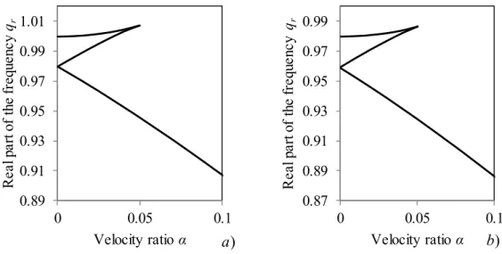
As already stated, it is seen in Figure 2 that, in some typical cases, there is only one positive real root for q ; three real roots for _r q exist for instance for low _r  and _N 0.2, as plotted in detail in Figure 3.

0.89 0.91 0.93 0.95 0.97 0.99 1.01 0 0.05 0.1 R ea l p ar t o f th e fr eq ue nc y qr Velocity ratio α 0.87 0.89 0.91 0.93 0.95 0.97 0.99 0 0.05 0.1 R ea l p ar t o f th e fr eq ue nc y qr Velocity ratio α

Figure 3: Detail of curves defining 0: a) _N 0.2, _S  , 0 _b  ; b) 0 _N 0.2, _S  , 0 0.2

b

 

In summary, the curves defining 0 can have several branches. Their separation at 0

r

q  can only occur for _b  and is given by 1





2 1 C b N S       and ₁ 2





C b N S        (59) C

 has no physical meaning, it marks a point where 0, but no associated branches are in the vicinity. _C marks the critical velocity when _b  . For this comparison the extended 0 formula for the critical velocity vcr ex, accounting for the normal force and the Pasternak

modulus must be considered





, 1

cr ex cr N S

v v    . (60)

If _b  , then 0 _C has no such meaning. It is not associated with the maximum beam deflection, even if the tendency is the same, i.e. the increase in damping decreases the value of _C and  at which the maximum beam deflection occurs.

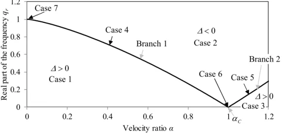
The nature of the roots p j_j, 1...4 of D p q is clarified in Figures 4 and 5. In Figure _r



, _r



4, the particular situation of _b  , 0 _N  , 0 _S  is shown. 0

)

17 0 0.2 0.4 0.6 0.8 1 1.2 0 0.2 0.4 0.6 0.8 1 1.2 R ea l p ar t o f th e fr eq ue nc y qr Velocity ratio α

Figure 4: Nature of the roots p jj, 1...4 of D p q as a function of r



, r



 and q . r

Case 7, reported in Figure 4, occurs only on some two-branches curves. For its existence it is necessary that _N _S. If _N _S, then Case 4 is extended from the first branch to the initial point with  0. When _N _S, then four-branches curve is formed, as shown in Figure 5 for _b  , 0 _N 0.2 and _S  . For better clarity, only the detail that is different 0 from Figure 4 is plotted.

0.89 0.91 0.93 0.95 0.97 0.99 1.01 0 0.05 0.1 R ea l p ar t o f th e fr eq ue nc y qr Velocity ratio α

Figure 5: Nature of the roots p jj, 1...4 of D p q as a function of r



, r



 and q . r

The cases reported in Figures 4 and 5 have the following meanings:

0  0  0  Case 1 Case 2 Case 3 Case 4 Case 5 Case 6 Case 7 Branch 1 Branch 2 C  Case 5 Case 5 Case 4 Case 3 Case 2 Case 1 Case 6 Case 8 Branch 1 Branch 3 Branch 4

18 Case 1: two pairs of complex conjugate roots

Case 2: two distinct real and two complex conjugate roots Case 3: four distinct real roots

Case 4: real double root and two complex conjugate roots Case 5: real double root and two distinct real roots

Case 6: two real double roots Case 7: quadruple real root

Case 8: triple real root and another distinct real root

To conclude this section, it is necessary to analyse, how K q behaves on complex

 

q -plane, when other parameters of the problem ( , _N, _S, _b) are fixed. Four q-values are considered in the form of: q_{ 1} q_ri



_bq_i



, q_{ 2} q_r i



_bq_i



, q_{ 3}   q_r i



_bq_i



and q_{ 4}   q_r i



_bq_i



, where q and _r q are real and positive. Then the _i D p q -



,



coefficients c and ₂ c are related by: ₃

 

 



 

 



2 2 2 1 * c q  c q , c q₂

 

_{ 4} 



c q₂

 

_{ 3}



*, c q₂

 

_{ 1}  c q₂

 

_{ 4} (61)  

 



 

 



3 2 3 1 * c q  c q , c q₃

 

_{ 4} 



c q₃

 

_{ 3}



*, c q₃

 

_{ 1} c q₃

 

_{ 4} (62) where the star designates the complex conjugate value. In these cases, D p q has complex



,



coefficients and thus four complex distinct roots. They fulfil

 

 

2



 

 1



* j j p q  p q , p q_j

 

_{ 4} 



p q_j

 

_{ 3}



*, p q_j

 

_{ 1}  p q_j

 

_{ 4} , j1,.., 4 (63) and therefore  

 

2



 

 1



* K q  K q , K q

 

_{ 4} 



K q

 

_{ 3}



*, K q

 

_{ 1} K q

 

_{ 4} (64) as follows from the sum of residues. This means that when q tends to zero, there is a _i discontinuity in Im K q



 



along the horizontal line in complex q-plane that cut the imaginary axis at i_b. Continuity is assured only in the case when Im



 



₀ 0

i

q

K q _  ,

which happens when _b  , 1   _C and q_r q_cut, where q is the value of _cut q lying on the _r first branch of 0 curve, because of the nature of the p-roots in the region. Existence of

C

 also requires that ₁ 2





₀

b N S

  

19

In summary, there is a discontinuity in K q , which means that branch cuts must be

 

introduced in the contour integration applied to Eq. (49) and (50). When _b  and 1





2

1_b  _N _S  , then for 0   _C the branch cuts can be reduced to run along i ,_b q_cut i_b

    and q_cuti ,_b  i_b . In all other cases full line i ,_b i_b

    must be considered.

At this moment, it looks like that it is exaggerating to use Cauchy’s residue theorem, because it seems to be easier just numerically integrate the Laplace image along

i ,a ia

    . But, as already highlighted in the Introduction, sum of residues will separate the oscillations into a finite number of harmonic vibrations, and consequently give clearer physical insight. It will be shown that the necessary input in form of induced frequencies can be determined quickly and accurately by the iteration techniques described in Section 3.4. All harmonic terms can be then expressed by analytical formulas that are not losing their precision with increasing time. Moreover, in the examples shown it will be seen that transient vibrations obtained by the numerical integration along the branch cuts have generally low influence, are rapidly decreasing, are numerically stable and in several cases can be neglected. This presents a clear advantage with respect to the full numerical integration along  i ,a  ia is numerically demanding for larger times and would not identify the unstable cases a priori. This also means that without knowing the poles, it is not clear what value for a should be used.

3.3 Solution in the time domain

From the analysis given in the previous section, one can conclude that the beam deflection shapes and the oscillator vibrations are given by

 



 

i



, , res i , e ,q W bc w   



W  q  q I_ (65)

 



 

i



, res i e ,q s U bc w  



U q  q I_ (66)

where the sum is performed over all residues and I_{W bc,} , I_{U bc,} stand for the results of the numerical integration along the branch cuts.

To evaluate the residues, it is necessary to determine the poles of iW

 

,q and iU q

 

. Both functions have the same denominator, thus the poles are the roots of Qq q



 f



with

20

Q given by Eq. (38). This expression has two obvious roots 0 and f, and others, designated

as induced frequencies, q , must be determined from _M Q0. By similar analysis as in the previous section, it can be concluded that if q₂  

 

q₁ * then K q

 

2 



K q

 

1



* and

 

2



 

1



*

Q q  Q q . Therefore, if

1

M

q is a root of Q0, then also





2 1 *

M M

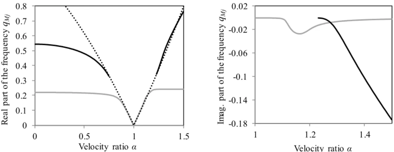
q  q is a root and thus the number of induced frequencies is even. This also indicates that a pair of induced frequencies have always the same imaginary parts and the opposite real parts. From the exponential form _eiq_{, it yields that the real parts of induced frequencies will form a harmonic}

function, while the imaginary parts will indicate whether the amplitude of the induced oscillation will gradually cease in time, will get unstable (gradually increase in time above all limits) or will stay unchanged, which will happen for the positive, negative and zero imaginary values, respectively.

In summary, the complete solution can be written as a sum of several terms: (i) steady-state terms corresponding to zero frequency, (ii) harmonic terms corresponding to excitation frequency, (iii) harmonic terms corresponding to induced frequencies and, (iv) transient terms corresponding to the integration along the branch cuts.

The steady-state terms are obtained as residues at q0

 

 





1 4 ,0 , K Pu Ps w          ₍₆₇₎

 

 





,1 4 0 2 _{s u} s P P P s s K w k           (68)

Both terms include the steady-state solution of the total constant force applied, P_u  . The P_s additional term in (68) stays for the static deflection of the oscillator spring caused by P , _s because ,1 2 ₂ 2 s P _{s u s} s st u s s s P k P P w w P k k k k  _   _   (69)

Terms in Eqs. (67) and (68) are stationary and only parameters entering the definition of



,



D p q with q0 are affecting the deflection value. Neither the harmonic force, nor the moving masses have any influence on this value, defined by the classical formula derived e.g. in [1]. Beam damping effect is also stationary.

21

 



_{ }



0  





i 3 / 2 2 i 2 4 , , e f 2 i e f s f P s s f M f f K w k c Q                       _{ }  (70)

 

_{ }

 

0  





i 3 /2 i ,2 4 e f 2 i e f f s P s s f f K w k c Q                 _{ }  (71) with

 



_{2 i}





₂

 





2



₂

 

4 2 u s s u s f s s f f M M f f M M f M f Q   k  c_    K      K           (72) Admitting only the moving mass, then

 





 

 



0



i 3 /2 i 2 ₂ 4 , e , e 2 f f u f P f M f K w K                      (73)

Eq. (73) reveals that there is generally another kind of resonance related to the excitation frequency, which occur for zero denominator in Eq. (73), or generally for zero value in Eq. (72). As the external frequency is real, this can only happen for c_s 0.

Expressions in Eqs. (70) and (71) define harmonic vibrations with the same frequency as the externally applied harmonic force. Besides the terms entering D p q with



,



q _f , it is seen that all other characteristics of the moving oscillator are affecting the amplitude value. Also here the damping effects of the beam and of the oscillator are stationary, and thus these oscillations theoretically last forever, as long as the external excitation is present.

Other harmonic terms are related to each calculated induced frequency, thus

 

0

j

M

Q q  .

The beam deflection shapes can be presented separately, for the constant and harmonic forces

 





  



2

 





i 3 , 4 , , j 2 i 2 i e _{M j} u j s j s j j j M q P s s M M M P s s M M q M K q w k c q q k c q q Q q            _{    (74)}

 







 

 



0 i 3 /2 2 i 4 , 4 , 2 i e , e f j j s j _{M j} j j P M s s M M M q q M M f K q k c q q w Q q q                _   (75)

The oscillator displacement in the same separation is

 





 





 





 

i 2 ,3 , 2 2 2 i 2 2 i e M j s j j u j u j j j j q P M s s M M M P M s s M s M q M K q k c q q K q k c q w q Q q                  ₍₇₆₎

 

 



 

 



0 i 3 /2 i ,4 , 4 2 i e e f j j _{M j} j j P M s s M q s q M M f K q k c q w Q q q            _   (77)

22 These expressions can be simplified for c_s 0

 













 

_





_

 

2 i 3 _{3 2 4} , 2 , , e 2 j u s u s j _{M j} j j s u j u s j s u j M s P P P M M q M q M M M M s M M M M M M s K q k q w q K q q k K q q k                           (78)

 





 

 

 









 

2 i ,3 _{3 2 4} , 2 2 e 2 s s u j s j u j _{M j} j j s u j u s j s u j P P P M s P M M M q s M q M M M M s M M M M M M s K q k K q q w q K q q k K q q k                            (79)

 







 

 









 



0







i i 3 /2 2 4 _{3 2 4} , 2 , e e , 2 M f j j j s j j j s u j u s j s u j j q M M s M M P M q M M M M s M M M M M M s M f q K q k q w q K q q k K q q k q                              (80)

 

 

 

 









 



0







i i 3 /2 ,4 _{3 2 4} , 2 e e 2 M f j j j j j s u j u s j s u j j q P M M s s M q M M M M s M M M M M M s M f q K q k w q K q q k K q q k q                          (81)

When only moving mass is considered, then

 





 

i 3 ₃ , 2 , , j u e _{M j} j j u M P q M q M M K q w q K q            ₍₈₂₎

 





 

 





0





i 3 /2 i 4 3 , 2 , e , e f j j _{M j} j u j j M M P q M M q M M f q K q w q K q q                  (83)

which is in agreement with [42]. The contributions of induced vibrations must be summed over all induced frequencies, even in numbers, as already mentioned. Here the damping effect is not stationary.

In the second part of this section, integration along the branch cuts to determine I_{W bc,} and

, U bc

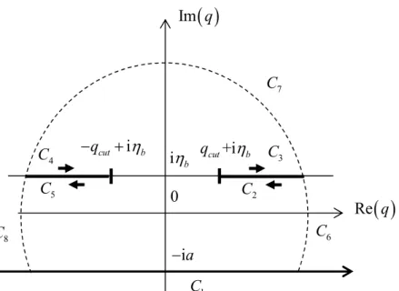
I_ is discussed. For simplicity, I where _C C  i ; ia    with a specified by the a inverse Laplace transform will designate the integral specified in Eqs. (49) or (50). Let _b  1 and   _C be assumed. According to Cauchy’s theorem of residues and by taking into account conclusions from Section 3.2, it holds:

1 2 i res 2 3 4 5 6 7 8 C C C C C C C C I  



I I I I I I I (84) where , 1,...,8 j C

I j stand for integrals along the contours identified by the subscript as represented in Figure 6. By analysing the functions W

   

,q / 2 and U q

   

/ 2 it can be concluded that they vanish for q   . Thus, when radius of the dashed contour in Figure 6 tends to infinity, 0

j

C

I  for j6,7,8 and also

1

C C

23

Figure 6: Schematic of the contour integration.

Then the term 2 i



res from Eq. (84) stand for



_{res i}



_W

 

_{,q e ,}iq _q



_and

 



i



res i_{U q} e ,q _q



 from Eqs. (65) and (66), respectively, and therefore



2 3 4 5



, C C C C

W bc

I_   I I I I with integrand equal to _W

 

_{,q e / 2}iq

 

_{ and}



2 3 4 5



, C C C C

U bc

I_   I I I I with integrand _{U q}

 

_{e / 2}iq

 

_ .

Some simplifications can be introduced. Having in mind the properties of K q analysed

 

in Section 3.2, it can be concluded that function values of both, _W

 

_{,q e / 2}iq

 

_{ and}

 

_{e / 2}iq

 

U q   at any point of C or ₂ C and for any ₃  and  are complex conjugate of function values at symmetrically located points at C or ₅ C , respectively, except for cases ₄ with external harmonic excitation. This property can significantly facilitate the numerical evaluation.

Nevertheless, although the roots of D p q have analytical expressions and until now



,



everything was presented analytically, an increased effort in providing better approach to integration along branch cuts than numerical, seems hard to justify, because this analytical expression would only be relatively complicated to integrate analytically. For the numerical evaluation of I_{W bc,} and I_{U bc,} , it is convenient to use a software of symbolic calculation with adjustable digits precision, like Maple. It is advantageous to prepare the function values along

0

 

Re q

 

Im q ia  i_b qcut+ib i cut b q    1 C 2 C 3 C 5 C 4 C 6 C 7 C 8 C

24

the branch cut in fixed points and then perform the sum representing the numerical integration for each  and  that is required. It is also helpful to visualize the function for  0, exploiting the analytical expressions of p-roots, to estimate the step for the numerical integration and the largest q-value that is necessary to consider. Then the numerical integration for calculation of I_{W bc,} and I_{U bc,} is straightforward and delivers numerically stable results. Transient vibrations obtained in this way have rapidly decreasing contribution to the full oscillator induced vibrations. This property is particularly noticeable in the subcritical region at the oscillator position.

3.4 Induced frequencies and evaluation of other necessary terms

The induced frequencies are the roots of Q0 given by Eq. (38). It was already proven, that pair of roots is linked by





2 1 *

M M

q  q . Moreover, when _b c_s 0, also

3 1

M M

q  q stand for a valid frequency, so as q_M4 

 

q_M1 *.

For better perception, it is useful to determine a variation of each induced frequency with respect to the velocity ratio  , when other data of the problem are fixed. Such curves will be named as frequency lines.

Two iterative techniques are proposed. From the numerical point of view, they only require repetitive calculation of K q . In the first one, the complex equation to be solved on complex

 

plane is written as if K q and

 

q were independent

 



,



0

Q q K q  (85)

If q is an estimate from n-th iteration, then the next iteration is calculated as _n





1 1

n i n

q _ q   q , where Q q K q



i,

 

n



0 (86)

This means that K q is evaluated at the previous estimate

 

q and then it is easy to solve _n

 



_i, _n



0

Q q K q  for q . Convergence of this technique depends on the initial estimate _i q ₀ and some adequate weight  . The initial estimate can be obtained from the general tendency of the frequency line. The iteration technique just described is usually convergent in full range of velocities with  0.5 and relatively high _b. If convergence difficulties are experienced,  should be reduced. This can happen close to the discontinuity in K q , i.e. when tested

 

frequencies have the imaginary parts near to _b. Other difficult region is in the vicinity of the

25

critical velocity, where Q q values have large variation. Then it is more convenient to use

 

the other proposed iteration method, named as delimiting search. For a reasonable estimate of the induced frequency value, it is possible to delimitate a rectangle domain in the complex q -plane where the real and imaginary parts of Q q are monotonic and change their sign. Zero

 

values mark two lines on the q-plane. In further iterations it is necessary to reduce the rectangle domain without losing the intersection of the lines just identified. By step-by-step reduction of the rectangle domain it is possible to determine the root with any required precision. For the purpose of this paper, both iterative techniques were programmed in Maple, in order to take advantage of the symbolic calculation and adjustable digits precision.

It is also possible to search for the roots by implementing the argument principle, but this is computationally more demanding. Nevertheless, the argument principle should always accompany previous calculations to confirm that all roots for given  have been found.

In the iterative techniques just introduced, repetitive calculation of K q for some fixed

 

q

is required. As already mentioned, K q can be determined by Cauchy’s residue theorem.

 

Due to the discontinuity of K q across the line with

 

Im

 

q  , frequency lines are _b interrupted when the corresponding imaginary part is infinitely close to _b. Therefore, K q

 

is only required at q for which D p q have four complex simple



,



p-roots. Then it is straightforward to select the ones with positive imaginary parts, for instance p and ₁ p to get ₂

 

_

_

_

_

1,2 , d 1 2 i , j p j, p K q D p q  D p q    







(87)

as given by the definition of the simple pole residue.

In the formulas of Section 3.3, besides K q , also

 

K_,q

 

q and K

 

,q are required for a given frequency q. K_,q

 

q has the same poles as K q , but all of them are duplicated, as

 

seen from

 

,

_



_



, 2 , d , q q D p q K q p D p q    

_

(88)

Then by implementation of the definition of the double pole residue







  

_{ }

   

   

 





2 2 6 2 d res , lim d ₃ z c g z g c h c g c h c f c z c z h z _{h c}         _  _    (89) one obtains

26

 



 



















2 2 , , , , , ₂ 2 1,2 , 6 , , 2 , , 2 i 3 , qp j pp j q j ppp j q j pp j D p q D p q D p q D p q K q D p q     



(90)

 

,

K  q is the only term that contains  and as such defines the full beam deflection shape. It can be again expressed analytically as the sum of residues. Poles are already known because they are the roots of D p q . In order to fulfil the boundary conditions from Eq. (15)



,



adapted to the dimensionless form, integration along positive infinite semicircle contour in the upper half-plane of the complex variable p must be used for the front wave and the negative value of the integration along the negative infinite semicircle contour in the lower half-plane of the complex variable p must be used for the rare wave.

4. Numerical examples

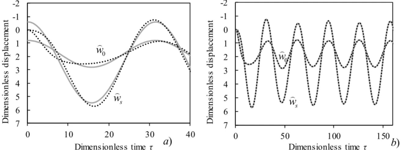
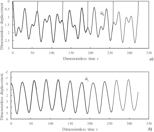
4.1 Validation and general remarks

All results presented in this section are validated by results obtained by modal expansion method on long finite beams. The resemblance of vibrations induced by moving loads on finite and infinite beams is notorious, when inertia of the moving object and reasonably stiff foundation are used, which is typical for railway applications. For the validation, the load has to be applied further from the support, to eliminate this influence. Then the choice of boundary conditions is immaterial and most convenient ones can be used, which in this case are simple supports that ensure analytically defined and numerically stable mode shapes. As mentioned above, it is also necessary to support the beam by a reasonably stiff foundation, to avoid higher displacements in the central beam sections. Then the vibrations obtained are independent on the beam length and thus can replace the results on infinite beam. This confirmation is presented in the first analysis of Section 4.2. For sufficient accuracy of results obtained by modal expansion method, high number of modes must be used as proven by convergence analysis in [42]. As expected, the necessary number of modes is increasing with the increasing beam length. All results on finite beams presented in this paper are sufficiently accurate, because they were tested for the number of modes, the initial distance of the oscillator from the support and the beam length. Further details about modal expansion method for simplified case of moving mass are given in [42]. Programs that calculate the beam and oscillator response are written in Matlab and were previously validated by commercial finite element software LS-DYNA. Validation by finite element results coming from LS-DYNA software is only possible in situations where the contact between the