Daniel Henrique Breda Binoti1, Mayra Luiza Marques da Silva Binoti2, Helio Garcia Leite3, Leonardo Fardin4, Julianne de Castro Oliveira5
(received: October 20, 2010; accepted: December 22, 2011)
ABSTRACT: The objective of this study was to evaluate the effectiveness of fatigue life, Frechet, Gamma, Generalized Gamma, Generalized Logistic, Log-logistic, Nakagami, Beta, Burr, Dagum, Weibull and Hyperbolic distributions in describing diameter distribution in teak stands subjected to thinning at different ages. Data used in this study originated from 238 rectangular permanent plots 490 m2 in size, installed in stands of Tectona grandis L. f. in Mato Grosso state, Brazil. The plots were measured at ages 34, 43, 55, 68, 81, 82, 92, 104, 105, 120, 134 and 145 months on average. Thinning was done in two occasions: the first was systematic at age 81months, with a basal area intensity of 36%, while the second was selective at age 104 months on average and removed poorer trees, reducing basal area by 30%. Fittings were assessed by the Kolmogorov-Smirnov goodness-of-fit test. The Log-logistic (3P), Burr (3P), Hyperbolic (3P), Burr (4P), Weibull (3P), Hyperbolic (2P), Fatigue Life (3P) and Nakagami functions provided more satisfactory values for the k-s test than the more commonly used Weibull function.
Key words: Teak, Weibull Distribution, thinning.
FUNÇÕES DENSIDADE DE PROBABILIDADE PARA DESCRIÇÃO DA DISTRIBUIÇÃO DIAMÉTRICA DE POVOAMENTOS DESBASTADOS DE Tectona grandis
RESUMO: Objetivou-se, neste trabalho, avaliar a eficiência das distribuições fatigue life, Frechet, gama, gama generalizada, logística generalizada, log-logística, Nakagami, beta, Burr, Dagum, Weibull e hiperbólica, para a descrição da distribuição diamétrica de povoamentos de teca submetidos a desbaste em diferentes idades. Os dados utilizados neste estudo foram provenientes de 238 parcelas permanentes retangulares de 490 m2 de área, instaladas em povoamentos de Tectona grandis L. f. no Estado do Mato Grosso, Brasil. As parcelas foram mensuradas, aos 34, 43, 55, 68, 81, 82, 92, 104, 105, 120, 134 e 145 meses em média. O povoamento foi desbastado em duas ocasiões, sendo o primeiro sistemático e aos 81 meses, com intensidade de 36% de área basal, e o segundo seletivo, removendo as piores árvores, aos 104 meses, em média, com redução de 30% de área basal. Os ajustes foram avaliados pelo teste de aderência Kolmogorov-Smirnorv. As funções Log-Logística (3P), Burr (3P), hiperbólica (3P), Burr (4P), Weibull (3P), Hyperbólica (2P), Fatigue Life (3P) e Nakagami, apresentaram valores para o teste k-s mais satisfatórios que a função comumente usada (Weibull).
Palavras-chave: Teca, Distribuição Weibull, desbaste.
1Forest Engineer, D.Sc. candidate in Forest Science – Departamento de Engenharia Florestal – Universidade Federal de Viçosa – 36570-000 – Viçosa, MG, Brasil – [email protected]
2Forest Engineer, Professor, D.Sc. candidate in Forest Science – Departamento de Engenharia Florestal – Universidade Federal de Viçosa – 36570-000 – Viçosa, MG, Brasil – [email protected]
3Forest Engineer, Professor, D.Sc. in Forest Science – Departamento de Engenharia Florestal – Universidade Federal de Viçosa – 36570-000 – Viçosa, MG, Brasil – [email protected]
4Forest Engineer – Floresteca – Av. Gov. João Ponce de Arruda, 1054 – 78110-375 – Várzea Grande, MT, Brasil – [email protected] 5Forest Engineer, M.Sc. candidate in Forest Science – Departamento de Engenharia Florestal – Universidade Federal de Viçosa – 36570-000 – Viçosa,
MG, Brasil – [email protected]
1 INTRODUCTION
Wood from Tectona grandis L. f. ranks high in the global market, particularly for the main intended purpose of furniture making, it being necessary to adopt thinning procedures in order to boost tree diameter for multiple
product applications, along with artificial pruning in order to obtain better quality wood in the final cutting process
(LEiTE et al., 2006).
a common characteristic in this type of modeling is the presence of a probability density function (pdf).
Different types of statistical distribution have already been used to describe diameter structure in forest stands, including: Gamma (NELSON, 1964), log-normal (BLiSS; rEiNKEr, 1965), Beta (CLUTTEr; BENNETT, 1965; PaLaHÍ et al., 2007), Johnson’s SB (HaFLEy; SCHUrEUDEr, 1977; PaLaHÍ et al., 2007), Hyper (LEiTE et al., 2009) and the Weibull distribution (BaiLEy; DELL, 1973; PaLaHÍ et al., 2007; WEiBULL, 1951). Since 1973, based on the study proposed by Bailey and Dell (1973), the Weibull function (MUrTHy et al., 2004) has been widely used in forestry (CaMPOS; TUrNBULL, 1981; CaO, 2004; CLUTTEr; aLLiSON, 1974; HaFLEy; SCHrEUDEr, 1977; KNOWE et al., 1997; MaTNEy; SULLiVaN, 1982; NOGUEira et al., 2005; PaLaHÍ et al., 2006, 2007).
a pdf may be fitted by methods of moments (FraziEr, 1981), percentiles (BaiLEy et al., 1989), maximum likelihood (FiSHEr, 1922), by combining methods of moments and percentiles (BaLDWiN JUNiOr; FEDUCCia, 1987), or by heuristic methods (aBBaSi et al., 2006, 2008).
Despite the prevalence of the Weibull pdf, statistical studies have presented new functions with
differing characteristics, flexibility and fitting capability.
Depending on the type of stand and horizontal structure found, other functions might result in greater accuracy. Therefore, this study aimed to assess the effectiveness of Fatigue life, Frechet, Gamma, Generalized Gamma, Generalized Logistic, Log-logistic, Nakagami, Beta, Burr, Dagum, Weibull and Hyperbolic distributions in describing diameter distribution in teak stands subjected to thinning at different ages.
2 MATERIAL AND METHODS
2.1 Data description
Data used in this study originated from 238 rectangular permanent plots 490 m2 in area, installed in
stands of Tectona grandis L. f. in Mato Grosso State, Brazil. These stands were located in a lowland region with geographical coordinates 15º 02’ to 15º 11’ south latitude and 56º 29’ to 56º 35’ west longitude, with initial spacing of 3.0 x 2.0 m. The average annual precipitation in the region is 1,300 to 1,600 mm, with six dry months, and the average annual temperature is 25.3 ºC.
The plots were measured at ages 34, 43, 55, 68, 81, 82, 92, 104, 105, 120, 134 and 145 months on average.
trees was measured 1.30 m above the ground (dbh). The
stand was thinned on two occasions, the first thinning
was systematic at 81months, with a basal area intensity of 36%, while the second was selective at 104 months and removed the poorer trees, reducing the basal area by 30% on average.
2.2 Probability Density Functions
For each plot and each measurement occasion, the
following functions were fitted:
- Beta (KriSHNaMOOrTHy, 2006)
1 2
1 2
1 1
1 1 2
1 ( ) ( )
( )
( , ) ( )
x a b x
f x
B b a
α α
α α α α
− −
+ −
− −
=
−
where
(
)
21
1
1 1
1 2 1, 2
0
( , ) 1 ( 0)
B α α = tα− −t α − dt α α >
∫
,1
α and α2are shape parameters (α α >1, 2 0), a, b are the
limits of the distribution (a<b)
- Fatigue Life (Birnbaum-Saunders) (JOHNSON et al., 1995)
(
)
(
)
(
)
1(
)
(
)
( )
2 x
x x
f x
x x
γ β
β γ γ β
φ
α γ α β γ
−
+
− −
= −
− −
where
( )
1 222 t
x e dt
π −
Φ =
∫
,( )
2
2
2 x e x φ
π −
= ,
α is the shape parameter
(
α >0)
,β is the scale parameter (β > 0), γ is the location parameter (γ ≡0, for a distribution with one parameter).- Frechet (BUry, 1999)
1
( ) x
f x e
x
α β α
γ
α β
β γ
+ − −
= −
where
- Gamma (KriSHNaMOOrTHy, 2006)
(
)
( )
1
( ) x x
f x e
α α γ γ β β α − − − = −
Γ
where
( )
1(
)
0
0 t
tα e dt
α ∞ − − α
Γ =
∫
>α is the shape parameter
(
α >0)
, β is the scale parameter (β > 0), γ is the location parameter (γ ≡0, for a distribution with two parameters)- Generalized Logistic (JOHNSON et al., 1995)
(
)
(
)
( )(
)
1 1 1 2 1 2 1 0 ... ... 1 1 ( ) ... 0 1 ... k z z az az f x e e α α β α β − − − − − + ≠ + + = = + where x y z β − =α is the shape parameter
(
α >0)
, β is the scale parameter (β > 0), γ is the location parameter (γ ≡0, for a distribution with two parameters)- Log-Logistic (JOHNSON et al., 1995)
2 1
( ) x 1 x
f x
α α
α γ γ
β β β
− − − − = + where
α is the shape parameter
(
α >0)
,β is the scale parameter (β > 0), γ is the location parameter (γ ≡0, for a distribution with two parameters)- Weibull (MUrTHy et al., 2004)
1
( )
x x
f x e
γ α γ β γ α β β − − − − = where
γ is the shape parameter
(
γ >0)
, β is the scale parameter (β > 0), α is the location parameter (α ≡0, for a distribution with two parameters)- Burr (JOHNSON et al., 1995)
1 1 ( ) 1 k x k f x x α α γ α β γ β β − + − = − + where
α and k are shape parameters
(
α >0)
, β is the scale parameter (β > 0), γ is the location parameter (γ ≡0, for a distribution with two parameters)- Generalized Gamma (JOHNSON et al., 1995)
1
( )
( ) exp( (( ) / ) )
( ) k
k k
k x y
f x β α αα x y β
− −
= − −
Γ
where
α and k are shape parameters
(
α >0)
, β is the scale parameter (β > 0), γ is the location parameter (γ ≡0, for a distribution with two parameters)- Nakagami (LaUrENSON, 1994)
2 1 2
2
( ) exp
( ) m
m m
m m
f x x x
m
−
= −
Ω
Γ Ω
where
m and Ω are constant parameters (m ≥ 0.5 and Ω > 0)
- Dagum (KLEiBEr; KOTz, 2003)
1 1 ( ) 1 k k x k f x x α α γ α β γ β β − + − = − + where
α and k are shape parameters
(
α >0)
, β is the scale parameter (β > 0), γ is the location parameter (γ ≡0, for a distribution with two parameters)- Hyperbolic (GUiMarãES, 2002)
( )
( )2 1
1
x x
f x tanh
α α
α γ γ
β β β
−
− −
= −
where
2.3 Function fitting and assessment
Dbh data from each plot and measurement occasion were grouped into class intervals of 1.0 cm. Functions were
fitted using the maximum likelihood method, with software kyplot Version 2.0 beta 15 (1997-2001c Koichi yoshioka).
Functions having a location parameter were fitted with
and without the parameter, as it can be replaced by the minimum diameter of the stand (CLUTTEr et al., 1983).
The following functions were thus fitted: Log-logistic (3P),
Log-logistic (2P), Burr (4P), Burr (3P), Hyperbolic (3P), Hyperbolic (2P), Weibull (3P), Weibull (2P), Fatigue Life (3P), Fatigue Life (2P) Nakagami, Gamma (3P), Gamma (2P), Generalized Gamma (4P), Generalized Gamma (3P), Generalized Logistic, Logistic, Frechet (3P), Frechet (2P), Beta, Dagum (4P), Dagum (3P), and numbers in brackets refer to the amount of parameters being used.
In order to test the goodness-of-fit of a function to
data, the Kolmogorov-Smirnov test was used (GiBBONS; SUBHaBraTa, 1992; SOKaL; rOHLF, 1981). This test compares estimated cumulative frequency with observed frequency, the maximum difference being the test statistic (dn). All fittings were compared through graphical analysis of observed and estimated values and mean values of the K-S test.
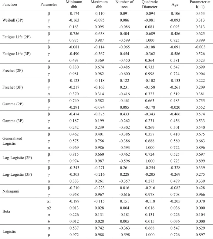
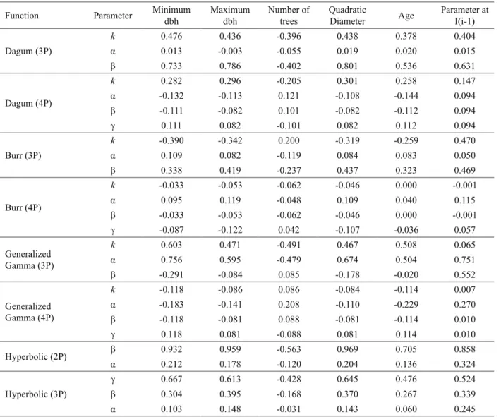
Considering that these functions are used in diameter distribution models and considering, in this case, the need
to obtain a significant correlation of their parameters
with the characteristics of the stands (LEiTE, 1990) a correlation matrix was estimated between the parameters and the variables: maximum diameter, minimum diameter, quadratic diameter, age, number of trees, also correlating parameter values at age i with an earlier age i-1.
3 RESULTS AND DISCUSSION
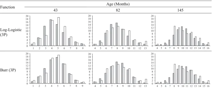
Functions were fitted to each plot and measurement occasion, to a total of 2,856 fittings per function. Graphical
analyses between estimated and observed values for three measurement occasions of a randomly selected plot are
provided in Figure 1. Function fit assessment was based
on K-S test values, the function providing the lowest mean values being considered the best function. results of the
K-S test for function fitting are provided in Table 1. Table
2 illustrates correlations between stand characteristics and functions parameters.
The diameter distribution modeling in stands of Tectona grandis L. f. (teak) has been performed based on the prediction and/or projection of parameters of a statistical distribution, using regression models. The two-parameter Weibull function has been used in the majority
of related studies on account of its flexibility and easy
correlation of its parameters with stand characteristics (NOGUEira et al., 2005).
Function age (Months)
43 82 145
Log-Logistic (3P)
0 2 4 6 8 10 12 14 16 18 20
1 2 3 4 5 6 7 8 9
0 2 4 6 8 10 12 14 16 18 20
4 5 6 7 8 9 10 11 12 13
0 2 4 6 8 10 12 14 16 18 20
4 5 6 7 8 9 10 11 12 13 14 15 16
Burr (3P)
0 2 4 6 8 10 12 14 16 18 20
1 2 3 4 5 6 7 8 9
0 2 4 6 8 10 12 14 16 18 20
4 5 6 7 8 9 10 11 12 13
0 2 4 6 8 10 12 14 16 18 20
4 5 6 7 8 9 10 11 12 13 14 15 16
To be continued...
Figure 1 – Observed values (in white) and estimated values (in gray) according to each tested function, for one plot in three measurement occasions.
Hyperbolic (3P) 0 2 4 6 8 10 12 14 16 18 20
1 2 3 4 5 6 7 8 9
0 2 4 6 8 10 12 14 16 18 20
4 5 6 7 8 9 10 11 12 13
0 2 4 6 8 10 12 14 16 18 20
4 5 6 7 8 9 10 11 12 13 14 15 16
Burr (4P) 0 2 4 6 8 10 12 14 16 18 20
1 2 3 4 5 6 7 8 9
0 2 4 6 8 10 12 14 16 18 20
4 5 6 7 8 9 10 11 12 13
0 2 4 6 8 10 12 14 16 18 20
4 5 6 7 8 9 10 11 12 13 14 15 16
Weibull (3P) 0 2 4 6 8 10 12 14 16 18 20
1 2 3 4 5 6 7 8 9
0 2 4 6 8 10 12 14 16 18 20
4 5 6 7 8 9 10 11 12 13
0 2 4 6 8 10 12 14 16 18 20
4 5 6 7 8 9 10 11 12 13 14 15 16
Hyperbolic (2P) 0 2 4 6 8 10 12 14 16 18 20
1 2 3 4 5 6 7 8 9 0 2 4 6 8 10 12 14 16 18 20
4 5 6 7 8 9 10 11 12 13
0 2 4 6 8 10 12 14 16 18 20
4 5 6 7 8 9 10 11 12 13 14 15 16
Fatigue Life (3P) 0 2 4 6 8 10 12 14 16 18 20
1 2 3 4 5 6 7 8 9
0 2 4 6 8 10 12 14 16 18 20
4 5 6 7 8 9 10 11 12 13
0 2 4 6 8 10 12 14 16 18 20
4 5 6 7 8 9 10 11 12 13 14 15 16
Nakagami 0 2 4 6 8 10 12 14 16 18 20
1 2 3 4 5 6 7 8 9
0 2 4 6 8 10 12 14 16 18 20
4 5 6 7 8 9 10 11 12 13
0 2 4 6 8 10 12 14 16 18 20
4 5 6 7 8 9 10 11 12 13 14 15 16
To be continued... Continua...
To be continued... Weibull (2P) 0 2 4 6 8 10 12 14 16 18 20
1 2 3 4 5 6 7 8 9
0 2 4 6 8 10 12 14 16 18 20
4 5 6 7 8 9 10 11 12 13
0 2 4 6 8 10 12 14 16 18 20
4 5 6 7 8 9 10 11 12 13 14 15 16
Gamma (2P) 0 2 4 6 8 10 12 14 16 18 20
1 2 3 4 5 6 7 8 9
0 2 4 6 8 10 12 14 16 18 20
4 5 6 7 8 9 10 11 12 13
0 2 4 6 8 10 12 14 16 18 20
4 5 6 7 8 9 10 11 12 13 14 15 16
Generalized Gamma (3P) 0 2 4 6 8 10 12 14 16 18 20
1 2 3 4 5 6 7 8 9
0 2 4 6 8 10 12 14 16 18 20
4 5 6 7 8 9 10 11 12 13
0 2 4 6 8 10 12 14 16 18 20
4 5 6 7 8 9 10 11 12 13 14 15 16
Generalized Logistic 0 2 4 6 8 10 12 14 16 18 20
1 2 3 4 5 6 7 8 9
0 2 4 6 8 10 12 14 16 18 20
4 5 6 7 8 9 10 11 12 13
0 2 4 6 8 10 12 14 16 18 20
4 5 6 7 8 9 10 11 12 13 14 15 16
Logistic 0 2 4 6 8 10 12 14 16 18 20
1 2 3 4 5 6 7 8 9
0 2 4 6 8 10 12 14 16 18 20
4 5 6 7 8 9 10 11 12 13
0 2 4 6 8 10 12 14 16 18 20
4 5 6 7 8 9 10 11 12 13 14 15 16
Gamma (3P) 0 2 4 6 8 10 12 14 16 18 20
1 2 3 4 5 6 7 8 9
0 2 4 6 8 10 12 14 16 18 20
4 5 6 7 8 9 10 11 12 13
0 2 4 6 8 10 12 14 16 18 20
4 5 6 7 8 9 10 11 12 13 14 15 16
Fatigue Life (2P) 0 2 4 6 8 10 12 14 16 18 20
1 2 3 4 5 6 7 8 9
0 2 4 6 8 10 12 14 16 18 20
4 5 6 7 8 9 10 11 12 13
0 2 4 6 8 10 12 14 16 18 20
4 5 6 7 8 9 10 11 12 13 14 15 16
Frechet (3P) 0 2 4 6 8 10 12 14 16 18 20
1 2 3 4 5 6 7 8 9
0 2 4 6 8 10 12 14 16 18 20
4 5 6 7 8 9 10 11 12 13
0 2 4 6 8 10 12 14 16 18 20
4 5 6 7 8 9 10 11 12 13 14 15 16
Beta 0 2 4 6 8 10 12 14 16 18 20
1 2 3 4 5 6 7 8 9
0 2 4 6 8 10 12 14 16 18 20
4 5 6 7 8 9 10 11 12 13
0 2 4 6 8 10 12 14 16 18 20
4 5 6 7 8 9 10 11 12 13 14 15 16
Dagum (3P) 0 2 4 6 8 10 12 14 16 18 20
1 2 3 4 5 6 7 8 9
0 2 4 6 8 10 12 14 16 18 20
4 5 6 7 8 9 10 11 12 13
0 2 4 6 8 10 12 14 16 18 20
4 5 6 7 8 9 10 11 12 13 14 15 16
Generalized Gamma (4P) 0 2 4 6 8 10 12 14 16 18 20
1 2 3 4 5 6 7 8 9
0 2 4 6 8 10 12 14 16 18 20
4 5 6 7 8 9 10 11 12 13
0 2 4 6 8 10 12 14 16 18 20
4 5 6 7 8 9 10 11 12 13 14 15 16
Dagum (4P) 0 2 4 6 8 10 12 14 16 18 20
1 2 3 4 5 6 7 8 9
0 2 4 6 8 10 12 14 16 18 20
4 5 6 7 8 9 10 11 12 13
0 2 4 6 8 10 12 14 16 18 20
4 5 6 7 8 9 10 11 12 13 14 15 16
To be continued... Continua...
Table 1 – Mean values of the Kolmogorov-Smirnov test for the tested functions. Numbers in brackets refer to the amount of parameters being used.
Tabela 1 – Média dos valores do teste Kolmogorov-Smirnov das funções testadas, para todos os ajustes. O valor entre parênteses refere-se ao número de parâmetros utilizado no ajuste.
p.d.f. Mean (K-S) p.d.f. Mean (K-S)
Log-logistic (3P) 0.1680 Generalized Logistic 0.1877
Burr (3P) 0.1690 Logistic 0.1887
Hyperbolic (3P) 0.1700 Gamma (3P) 0.1887
Burr (4P) 0.1709 Fatigue Life (2P) 0.1962
Weibull (3P) 0.1710 Frechet (3P) 0.2014
Hyperbolic (2P) 0.1722 Beta 0.2014
Fatigue Life (3P) 0.1737 Dagum (3P) 0.2020
Nakagami 0.1794 Generalized Gamma (4P) 0.2139
Weibull (2P) 0.1800 Dagum (4P) 0.2678
Gamma (2P) 0.1855 Log-logistic (2P) 0.3286
Generalized Gamma (3P) 0.1868 Frechet (2P) 0.3993 Log-Logistic
(2P)
0 2 4 6 8 10 12 14 16 18 20
1 2 3 4 5 6 7 8 9
0 2 4 6 8 10 12 14 16 18 20
4 5 6 7 8 9 10 11 12 13 0 2 4 6 8 10 12 14 16 18 20
4 5 6 7 8 9 10 11 12 13 14 15 16
Frechet (2P)
0 2 4 6 8 10 12 14 16 18 20
1 2 3 4 5 6 7 8 9
0 2 4 6 8 10 12 14 16 18 20
4 5 6 7 8 9 10 11 12 13
0 2 4 6 8 10 12 14 16 18 20
4 5 6 7 8 9 10 11 12 13 14 15 16
Table 2 – Correlation between stand characteristics and function parameters.
Tabela 2 – Correlação entre características do povoamento e os parâmetros das funções ajustadas.
Function Parameter Minimum dbh
Maximum dbh
Number of trees
Quadratic
Diameter age
Parameter at i(i-1)
Weibull (2P) β 0.803 0.649 -0.451 0.717 0.512 0.698
γ 0.967 0.990 -0.592 1.000 0.724 0.892
To be continued...
Table 2 – Continued... Tabela 2 – Continuação...
Function Parameter Minimum dbh
Maximum dbh
Number of trees
Quadratic
Diameter age
Parameter at i(i-1)
Weibull (3P)
β -0.174 -0.110 0.091 -0.094 -0.106 0.353
γ -0.163 -0.095 0.086 -0.081 -0.093 0.313
α 0.163 0.095 -0.086 0.081 0.093 0.313
Fatigue Life (2P) β -0.756 -0.638 0.404 -0.689 -0.486 0.625
γ 0.975 0.987 -0.599 1.000 0.725 0.899
Fatigue Life (3P)
β -0.081 -0.114 -0.065 -0.108 -0.091 -0.003
γ -0.490 -0.367 0.454 -0.362 -0.586 0.526
α 0.493 0.369 -0.450 0.364 0.581 0.523
Frechet (2P) β 0.830 0.674 -0.485 0.733 0.547 0.699
γ 0.981 0.982 -0.600 0.998 0.724 0.904
Frechet (3P)
β -0.123 -0.118 0.122 -0.102 -0.133 0.222
γ -0.217 -0.163 0.231 -0.158 -0.261 0.209
α 0.370 0.314 -0.416 0.323 0.519 0.381
Gamma (2P) β 0.740 0.582 -0.461 0.663 0.485 0.755
γ -0.291 -0.084 0.085 -0.178 -0.020 0.552
Gamma (3P)
β -0.474 -0.375 0.433 -0.343 -0.466 0.574
γ 0.187 0.199 -0.262 0.231 0.456 0.533
α 0.242 0.239 -0.302 0.269 0.501 0.540
Generalized Logistic
β 0.462 0.401 -0.386 0.357 0.410 0.675
γ 0.575 0.756 -0.386 0.688 0.580 0.663
α 0.969 0.986 -0.593 1.000 0.722 0.896
Log-Logistic (2P) β 0.815 0.660 -0.462 0.724 0.525 0.697
γ 0.974 0.987 -0.596 1.000 0.723 0.899
Log-Logistic (3P)
β -0.343 -0.271 0.261 -0.254 -0.328 0.339
γ -0.303 -0.216 0.228 -0.205 -0.269 0.275
α 0.333 0.261 -0.357 0.273 0.479 0.339
Nakagami β -0.210 -0.223 0.016 -0.216 -0.082 0.428
γ 0.958 0.967 -0.616 0.978 0.708 0.966
Beta
α1 -0.199 -0.115 0.151 -0.118 -0.205 0.070
α2 0.013 0.028 0.004 0.016 0.036 0.000
a 0.226 0.131 -0.181 0.131 0.226 0.104
b 0.012 0.028 0.005 0.015 0.036 0.000
Logistic σ 0.537 0.742 -0.363 0.668 0.547 0.629
μ 0.972 0.988 -0.598 1.000 0.726 0.897
Table 2 – Continued... Tabela 2 – Continuação...
Function Parameter Minimum dbh
Maximum dbh
Number of trees
Quadratic
Diameter age
Parameter at i(i-1)
Dagum (3P)
k 0.476 0.436 -0.396 0.438 0.378 0.404
α 0.013 -0.003 -0.055 0.019 0.020 0.015
β 0.733 0.786 -0.402 0.801 0.536 0.631
Dagum (4P)
k 0.282 0.296 -0.205 0.301 0.258 0.147
α -0.132 -0.113 0.121 -0.108 -0.144 0.094
β -0.111 -0.082 0.101 -0.082 -0.112 0.094
γ 0.111 0.082 -0.101 0.082 0.112 0.094
Burr (3P)
k -0.390 -0.342 0.200 -0.319 -0.259 0.470
α 0.109 0.082 -0.119 0.084 0.083 0.050
β 0.338 0.419 -0.237 0.437 0.323 0.469
Burr (4P)
k -0.033 -0.053 -0.062 -0.046 0.000 -0.001
α 0.095 0.119 -0.048 0.109 0.040 0.115
β -0.033 -0.053 -0.062 -0.046 0.000 -0.001
γ -0.087 -0.122 0.042 -0.107 -0.036 0.057
Generalized Gamma (3P)
k 0.603 0.471 -0.491 0.467 0.508 0.065
α 0.756 0.595 -0.479 0.674 0.504 0.751
β -0.291 -0.084 0.085 -0.178 -0.020 0.552
Generalized Gamma (4P)
k -0.118 -0.086 0.086 -0.084 -0.114 0.007
α -0.183 -0.141 0.208 -0.110 -0.229 0.270
β -0.118 -0.081 0.088 -0.081 -0.114 0.010
γ 0.118 0.081 -0.088 0.081 0.114 0.010
Hyperbolic (2P) β 0.932 0.959 -0.563 0.969 0.705 0.858
α 0.212 0.178 -0.120 0.204 0.136 0.324
Hyperbolic (3P)
γ 0.667 0.613 -0.428 0.645 0.476 0.524
β 0.304 0.395 -0.168 0.370 0.267 0.339
α 0.103 0.148 -0.031 0.143 0.060 0.245
The effectiveness of estimates generated by diameter distribution models is conditional not only on data
quality and equation fitting quality but also on correlation
capability between pdf parameters and easily measurable stand characteristics (LEiTE, 1990).
This study evaluated the application of functions with differing characteristics to describe the diameter structure of teak stands subjected to thinning. The Log-Logistic (3P), Burr (3P), Hyperbolic (3P), Burr (4P), Weibull (3P), Hyperbolic (2P), Fatigue Life (3P) and Nakagami functions provided more satisfactory values for
Nevertheless, all functions being analyzed in this study provided satisfactory results for use in growth and yield modeling of thinned teak stands.
among the tested functions, the hyperbolic function, as proposed by Guimarães (2002) and used in this study, has great potential to describe diameter
distribution of forest stands on account of its flexibility. The inflection point of this function ranges from zero to the upper limit defined by I = tanh(1) = 0.76. This
confers greater flexibility in comparison with the Weibull function, whose inflection points range between zero and
the limit of i = (1-1/e) = 0.63. Thus, the characteristic given by many authors to justify using the Weibull function to describe diameter structure in thinned stands is even more substantial in the case of the hyperbolic function. in addition, the parameters of this function are easily correlated with stand characteristics, as was observed by Campos e Leite (2009) and Leite et al. (2010).
Functions were fitted using the maximum likelihood method only. Other fitting methods should be tested that
include percentiles method (GUiMarãES, 1994), methods of moments (FraziEr, 1981) and moments-l in order to determine how best to use each function.
4 CONCLUSION
This study demonstrated that, other than the Weibull function, other functions can be used to describe the diameter structure of stands subjected to thinning, potentially resulting in greater accuracy than the more commonly used Weibull function, noting that they should also be tested with other types of stand.
5 REFERENCES
aBBaSi, B.; JaHrOMia, a. H. E.; arKaT, J.; HOSSEiNKOUCHaCK, M. Estimating the parameters of Weibull distribution using simulated annealing algorithm.
Applied Mathematics and Computation, New york, v. 183, n. 1, p. 85-93, Mar. 2006.
aBBaSi, B.; raBELO, L.; HOSSEiNKOUCHaCK, M. Estimating parameters of the three-parameter Weibull distribution using a neural network. European Journal
of Industrial Engineering, Oxford, v. 2, n. 4, p. 428-445, 2008.
BaiLEy, r. L.; BUrGaN, T. M.; JOKELa, E. J. Fertilized midrotation-aged slash pine plantations: stand structure and yield prediction models. Southern Journal of Applied Forestry, Washington, v. 13, n. 2, p. 76-80, 1989.
BaiLEy, r. L.; DELL, T. r. Quantifying diameter distributions with the Weibull function. Forest Science, Bethesda, v. 19, n. 2, p. 97-104, 1973.
BaLDWiN JUNiOr, V. C.; FEDUCCia, D. P. Loblolly
pine growth and yield prediction of managed West Gulf
plantations. New Orleans: USDa, 1987. 27 p.
BLiSS, C. L.; rEiNKEr, K. a. a lognormal approach to diameter distributions in even-aged stands. Forest Science, Bethesda, v. 10, p. 350-360, 1964.
BUry, K. Statistical distributions in engineering. Cambridge: Cambridge University, 1998. 362 p.
CaMPOS, J. C. C.; LEiTE, H. G. Mensuração florestal: perguntas e respostas. 3. ed. Viçosa, MG: UFV, 2009. 548 p.
CaMPOS, J. C. C.; TUrNBULL, K. Um sistema para estimar a produção por classe de diâmetro e sua aplicação na interpretação do efeito de desbaste. Revista Árvore, Viçosa, v. 5, n. 1, p. l-l6, 1981.
CaO, Q. V. Predicting parameters of a Weibull function for modeling diameter distribution. Forest Science, Oxford, v. 50, n. 4, p. 682-685, 2004.
CLUTTEr, J. L.; aLLiSON, B. J. a growth and yield model for Pinus radiata in New zealand for tree and stand simulation.
Royal College of Forestry, London, n. 30, p. 136-160, 1974.
CLUTTEr, J. L.; BENNETT, F. a. Diameter distributions in
old: field slash pine plantations. Georgia Forest Research
Council Report, Maple, n. 13, p. 1-9, 1965.
CLUTTEr, J. L.; FOrTSON, J. C.; PiENaar, L. V.; BriSTEr, r. G. H.; BaiLEy, r. L. Timber management: a quantitative approach. New york: J. Willey, 1983. 333 p.
FiSHEr, r. a. On the mathematical foundations of theoretical statistics. PhilosophicalTransactions of the Royal Society of London, Serie A, London, v. 222, p. 309-368, 1922.
FraziEr, J. r. Compatible whole-stand and diameter
GiBBONS, J. D.; SUBHaBraTa, C. Nonparametric statistical inference. 3. ed. New york: M. Dekker, 1992. 544 p.
GUiMarãES, D. P. Desenvolvimento de um modelo de
distribuição diamétrica de passo invariante para prognose e projeção da estrutura de povoamentos de eucalipto. 1994. Tese (Doutorado em Ciência Florestal) - Universidade Federal de Viçosa, Viçosa, 1994.
GUiMarãES, D. P. Uma função hiperbólica de
distribuição probabilística de alta flexibilidade. Planaltina: Embrapa Cerrados, 2002. 40 p.
HaFLEy, W. L.; SCHrEUDEr, H. T. Statistical distributions
for fitting diameter and height data in ever-aged stands.
Canadian Journal of Forest Research, Ottawa, v. 7, p. 184-487, 1977.
JOHNSON, N. L.; KOTz, S.; BaLaKriSHNaN, N. Continuous univariatedistributions. New york: applied Probability and Statistics, 1995. 732 p.
KLEiBEr, C.; KOTz, S. Statistical size distributions in
economics and actuarialsciences. New york: J. Wiley, 2003. 353 p.
KNOEBELL, B. r.; BUrKHarT, H. E.; BECK, D. E. a growth and yield model for thinned stands of yellow-poplar. Forest Science, Oxford, v. 32, n. 2, p. 62, 1986.
KNOWE, S. a.; aHrENS, G. a.; DEBELL, D. S.
Comparison of diameter-distribution -prediction, stand-table -projection and individual-tree growth modeling approaches for young red alder plantations. Forest Ecology and
Management, amsterdam, v. 96, p. 207-216, 1997.
KriSHNaMOOrTHy, K. Handbook of statistical
distributions withapplications. London: Taylor & Francis, 2006. 346 p. (Statistics, a series of textbooks & monographs, 188).
LaUrENSON, D. Nakagami distribution: indoor radio channel propagation modelling by ray tracing techniques. [S.l.: s.n.], 1994.
LEiTE, H. G. Ajuste de um modelo de estimação de
freqüência e produção por classe de diâmetro, para povoamentos de Eucalyptus saligna Smith. 1990. 81 f. Dissertação (Mestrado em Ciência Florestal) - Universidade Federal de Viçosa, Viçosa, 1990.
LEiTE, H. G.; BiNOTi, D. H. B.; GUiMarãES, D. P.; SiLVa, M. L. M.; GarCia, S. L. r. avaliação do ajuste das funções Weibull e hiperbólica a dados de povoamentos de eucalipto submetidos a desbaste. Revista Árvore, Viçosa, v. 34, n. 2, p. 220-226, 2010.
LEiTE, H. G.; NOGUEira, G. S.; CaMPOS, J. C. C.; TaKizaWa, F. H.; rODriGUES, F. L. Um modelo de distribuição diamétrica para povoamentos de Tectona grandis submetidos a desbaste. Revista Árvore, Viçosa, v. 30, n. 1, p. 89-98, 2006.
MaTNEy, T. G.; SULLiVaN, a. D. Variable top volume and height predictions for slash pine trees. Forest Science, Bethesda, v. 28, n. 2, p. 74-82, 1982.
MUrTHy, D. N. P.; XiE, M.; JiaNG, r. Weibull models. New york: Wiley, 2004. 396 p.
NELSON, T. C. Diameter distribution and growth of loblolly pine. Forest Science, Bethesda, v. 10, n. 1, p. 105-114, 1964.
NOGUEira, G. S.; LEiTE, H. G.; CaMPOS, J. C. C.; CarVaLHO, a. F.; SOUza, a. L. de. Modelo de distribuição diamétrica para povoamentos de Eucalyptus sp. submetidos a desbaste. Revista Árvore, Viçosa, v. 29, n. 4, p. 579-589, jul./ ago. 2005.
SiiPiLEHTO, J.; SarKKOLa, S.; MEHTÄTaLO, L. Comparing regression estimation techniques when predicting diameter distributions of Scots pine on drained peatlands. Silva Fennica, Helsinski, v. 41, n. 2, p. 333-349, 2007.
SOKaL, r. r.; rOHLF, F. J. Biometry. San Francisco: Freeman, 1981. 859 p.