Computer simulation of a Rietema-family hydrocyclone used in
irrigated agriculture
1Simulação computacional de Hidrociclone da família Rietema aplicado na agricultura
irrigada
Paulo César Tonin2*, José Dantas Neto3 e José Airton Azevedo dos Santos4
ABSTRACT - The hydrocyclone is a centrifugal separator that has been used for over 50 years in the chemical processing and mining industries. In irrigated agriculture in Brazil it is not used as often. One reason for this is the poor understanding by designers of the complex phenomena involved in the internal flow of the hydrocyclone, and the lack of knowledge of new computational tools available on the market. This study evaluates the use of Computational Fluid Dynamics (CFD) as a potential tool to be used in the design and optimisation of hydrocyclones used in irrigated agriculture. A 50 mm Rietema-family hydrocyclone is simulated using CFD. The turbulent flow inside the hydrocyclone is modelled using the Reynolds Stress Model, and a Eulerian approach is employed to model the multiphase flow. Numeric validation is performed by comparing the results of the simulation with data found in the literature. The global mass balance observed for both the single-phase and multiphase flows shows good agreement of the obtained results with data in the literature. Furthermore, the static pressure field, the axial and tangential velocity and the volume fraction of sediments in the hydrocyclone are obtained. The article shows that CFD is a useful tool in explaining the process of sediment separation in the hydrocyclone, and can therefore be used in the design and optimisation of such equipment.
Key words: Pre-filtering. Computational fluid dynamics. Multiphase flow. Particle size.
RESUMO - O hidrociclone é um separador centrífugo que vem sendo utilizado a mais de 50 anos nas indústrias de processamento químico e de mineração. Na agricultura irrigada no Brasil ele não é utilizado com a mesma frequência. Um dos fatores para isto é o pouco entendimento, por parte dos projetistas, dos complexos fenômenos envolvidos no escoamento interno dos hidrociclones e no desconhecimento de novas ferramentas computacionais disponíveis no mercado. Neste estudo avalia-se o uso da Dinâmica dos Fluidos Computacional (CFD), como uma ferramenta potencial, a ser usada no projeto e otimização de hidrociclones aplicados à agricultura irrigada. Um hidrociclone da família Rietema de 50 mm é simulado utilizando a CFD. O escoamento turbulento dentro do hidrociclone é modelado utilizando o modelo Reynolds Stress Model e o escoamento multifásico é modelado através de uma abordagem Euleriana. A validação numérica é feita comparando os resultados da simulação com dados presentes na literatura. Os balanços de massas globais observados tanto para o escoamento monofásico quanto para o multifásico mostram uma boa concordância dos resultados obtidos com os dados presentes na literatura. Além disto, o campo de pressão estática, a velocidade axial e tangencial, e a fração em volume dos sedimentos dentro do hidrociclone são obtidos. O artigo mostra que a CFD é uma ferramenta útil em explicar o processo de separação dos sedimentos no hidrociclone e pode, portanto ser utilizada no projeto e otimização destes equipamentos.
Palavras-chave: Pré-filtragem. Dinâmica dos fluidos computacional. Escoamento multifásico. Tamanho de partícula.
*Autor para correspondência
1Recebido para publicação em 13/03/2013; aprovado em 15/10/2014
Parte da Tese de Doutorado do primeiro autor, apresentado ao programa de Pós-Graduação em Irrigação e Drenagem, Universidade Federal de Campina Grande
2Departamento de Manutenção Industrial, Universidade Tecnológica Federal do Paraná/UTFPR, Medianeira-PR, Brasil, pctonin@utfpr.edu.br 3Departamento de Engenharia Agrícola, Universidade Federal de Campina Grande, Campina Grande-PB, Brasil, zedantas@deag.ufcg.edu.br 4Departamento de Engenharia de Produção, Universidade Tecnológica Federal do Paraná/UTFPR, Medianeira-PR, Brasil, professorjairton@
INTRODUCTION
Hydrocyclones are used in irrigation and have the function of separating sediments suspended in the water, thus avoiding a decrease in the efficiency and useful life of the system. While easy to build, the internal flow of a hydrocyclone is very complex and poorly understood due to the high turbulence and vorticity, fundamental parameters that the designer must be aware of in order to construct the best equipment.
In the last two decades Computational Fluid Dynamics (CFD) has been used in simulations of complex flow, and large gains, such as lower development costs and increases in operational performance, have been achieved with its use. Although widely used by other sectors of industry, CFD is still little applied in the simulation and prediction of the performance of hydrocyclones, especially those used in irrigated agriculture.
The most critical aspect of CFD simulation in hydrocyclones is the choice of turbulence model, (DARMANWAN; TADE; EVANS, 2011). Some of these models, such as the k- and Re-Normalisation Group (RNG-k- ), have been studied and evaluated by several authors in the last two decades (CULLIVAN; WILLIAMS; CROSS, 2003; CULLIVAN et al., 2004; DYAKOWSKI; WILLIAMS, 1995; GRADY
et al., 2002; NOWAKOWSKI; DYAKOWSKI, 2003;
NOWAKOWSKI et al., 2004; SCHUETZ et al., 2004). A high-order turbulence model known as the Reynolds Stress Model (RSM) was used by the authors (BRENNAN, 2006; NARASIMHA; BRENNAN; HOLTHAM, 2006; WANG; CHU; WU, 2007). As a result, the velocity profile was predicted, and comparison with the experimental data showed good agreement for all the studies.
Computer simulations involving multiphase flow (air-liquid-solid) for hydrocyclones used in mining, have been carried out by several authors (HSU; WU; WU, 2011; MOTSAMAI, 2010; SHOJAAEEFARD; NOORPOOR; HABIBIAN, 2009; WANG; YU, 2006; ZHANG; YOU; NIU, 2011). Turbulent flow has been modelled using the Reynolds Stress Model (RSM), and the flow of particles described by the Eulerian and/or Lagrangian models. All studies have shown that efficiency in separating the sediment is highly influenced by the geometrical dimensions of the hydrocyclone.
This article aims to evaluate the use of CFD as a potentially useful tool to be employed in the design and optimisation of hydrocyclones used in irrigated agriculture.
MATERIAL AND METHODS
Description of the mathematical models
The multiphase flow conservation equations (Navier-Stokes) are written in a generalised way. In the Eulerian model, these Reynolds-averaged equations are:
(1)
(2)
where: subscript is the generic phase (solid or liquid); is the density of the generic phase ; t represents time and
is the viscosity. Finally, v represents the velocity vector, defined by the average Reynolds equation as:
(3)
In equation (2) the term represents the Reynolds stress tensor.
These equations apply to a hydrocyclone with incompressible and transient flows in 3D coordinate systems. The energy conservation equation is not considered, as the flow may be regarded as almost isothermal.
The RSM turbulence model closes the Navier-Stokes equations, using Reynolds averaging for solving the transport equations for the Reynolds tensors, together with an equation for the rate of dissipation. This means that five additional transport equations are required in 2D flow and seven additional transport equations must be solved in 3D flow, Versteeg and Malalasekera (1995).
According to the RSM model, the Reynolds tensors can be modelled by the following equation:
(4)
The term for stress production is given by:
(5)
The term Øij is the deformation due to pressure, one of the most important terms in the model, being divided into two parts:
Øij= Øij,1+Øij,2 (6)
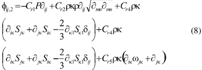
For the model used in this work they are defined as:
(8)
As the term for turbulence dissipation still appears in the individual tensor equations, a new transport equation is required:
(9)
where: k is the turbulent kinetic energy; is the dissipation of the turbulent kinetic energy; is the turbulent viscosity; Sv
1
x,y,zrepresents the source term along the x, y and z axes
for the liquid or solid phase; is the anisotropic tensor; is the Kronecker delta function and is a global scalar variable. The constants used in the above equations are:
C = 0,22; C1 = 1,7; C2 = -1,05; Cr1 = 0,9; Cr2 = 0,8; Cr3 = 0,65; Cr4 = 0,625; Cr5 = 0,2; = 1,3; and were taken from the ANSYS® CFX® 13.0 software.
Figure 1 - (a) Constituent parts (b) Dimensions of the hydrocyclone
Simulation and experimental conditions
The constituent parts and geometrical parameters of the hydrocyclone used in this simulation are the same used by Soccol (2004), and can be seen in Figure 1a and 1b respectively.
The geometrical parameters are: diameter of the cylindrical portion (Dc = 50 mm), diameter of the feed tube (Da = 14 mm), the diameter of the diluent tube (Do = 18 mm), diameter of the concentrated suspension outlet orifice (Du = 10 mm), length of the cylindrical portion (Lk = 65 mm), length of the diluent tube (l = 20 mm), cone length (Le = 185 mm) and cone angle (A = 12.34º). These parameters according to Svarovsky (1984), characterise the separation efficiency, pressure drop and separation ratio of a hydrocyclone.
To ensure the independence of the obtained result in relation to the adopted mesh-density, a test was initially held with five meshes of different densities: 50,000; 100,000; 120,000; 180,000 and 240,000 tetrahedral elements.
A mesh density of 180,000 elements was chosen as this gives good solutions with reasonable computer time, Figure 2.
Figure 2 - Density of a mesh of 180,000 elements
found in the ANSYS® CFX® 13.0 commercial software. The coupling between pressure and velocity is solved implicitly by the Semi Implicit Linked Equation algorithm (SIMPLEC). The SIMPLEC procedure describes the pressure as the sum of the best estimate for available pressure P* and a correction P’, which is calculated in such a way as to satisfy the continuity equation, i.e.
P = P* + P` (10)
With the pressure field estimated, the equations for the Conservation of Momentum are calculated; it is then necessary to correct the velocities so that these satisfy the equation for the Conservation of Mass. To do this, the speed correction equations must be determined, their quality significantly influencing the rate of convergence of the iterative process. The pressures are then increased in order to complete the iterative cycle. In all the numerical experiments the convection terms of the partial differential equations are discretised using the second-order upwind scheme. In this scheme the quantities on the faces of the control volumes are calculated by a linear and multidimensional reconstruction approximation. Second order accuracy is achieved on the faces of the control volumes through the expansion by Taylor series of the solution centered on the control volume in relation to its centroid:
(11)
where, Ø e Ø are the values at the centre of the control volume and its gradient upstream in the control volume respectively, and is the displacement vector from the centroid of the upstream control volume to the centroid of the face.
To save time in the simulations, results converged by the k-e model were used as an initial solution for the RSM model. A time step of 0.025 s and a total simulation time of 3 sec were used. A transient simulation was performed with 5 interactions for each time step. A convergence criterion of 10-6 was adopted for the residual iterations of the transport equations.
Table 1 - Physical properties of the water
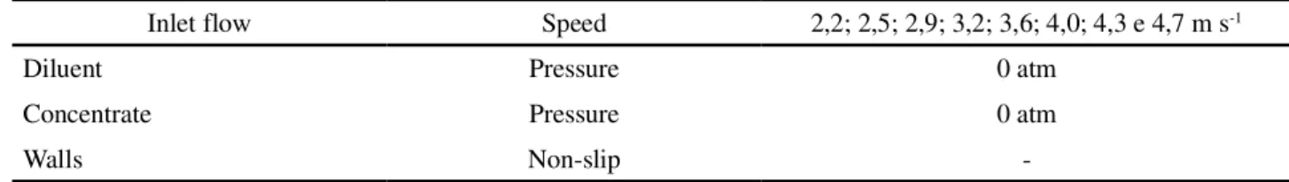
Table 2 - Boundary Conditions
Type of fluid Water
Specific weight 997 km m-3
Dynamic viscosity 8,899 x 10-4 kg m-1s-1
Specific heat at constant pressure 4181,7 J kg-1k-1
Temperature 22 ºC
Inlet flow Speed 2,2; 2,5; 2,9; 3,2; 3,6; 4,0; 4,3 e 4,7 m s-1
Diluent Pressure 0 atm
Concentrate Pressure 0 atm
-Figure 3 - Pressure drop vs. water inlet velocity
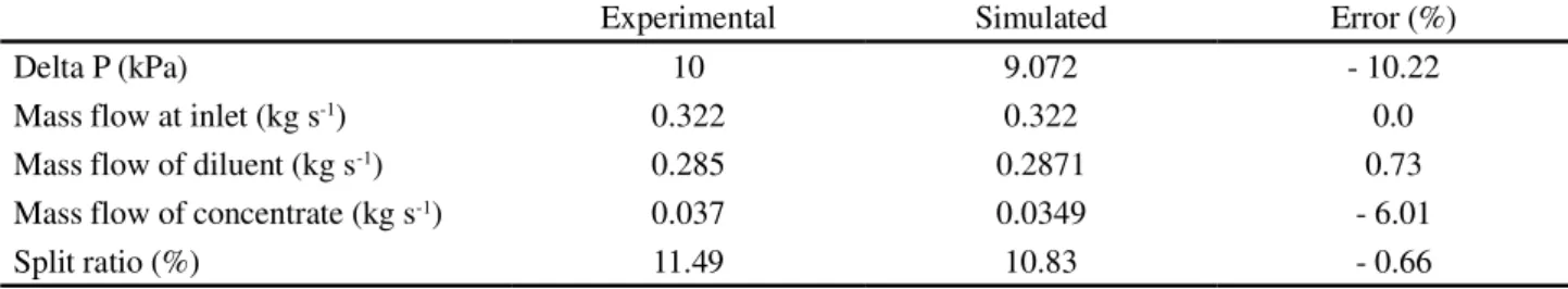
Table 3 - Global mass balance for single-phase flow
RESULTS AND DISCUSSION
Validation of the Model
For single-phase flow, the simulations were carried out with an aim to evaluate the RSM turbulence model, indicated in the literature as one of the models that is better able to predict the anisotropic flow characteristic of hydrocyclones. The physical properties of the water and the boundary conditions used in the simulations can be seen in Tables 1 and 2 respectively.
The results obtained in this simulation are compared with the Soccol experimental data (2004) and shown in Figure 3.
It is seen from Figure 3 that the RSM turbulence model was able to closely predict the pressure drop, with deviations of the order of -10 to -15% when the inlet velocity was 2.2 and 4.7 m s-1 respectively. The mean square error between the experimental data and
Experimental Simulated Error (%)
Delta P (kPa) 10 9.072 - 10.22
Mass flow at inlet (kg s-1) 0.322 0.322 0.0
Mass flow of diluent (kg s-1) 0.285 0.2871 0.73
Mass flow of concentrate (kg s-1) 0.037 0.0349 - 6.01
Split ratio (%) 11.49 10.83 - 0.66
the values obtained with the model is 20.02. The overall mass balance, considering an inlet velocity of 2 m s-1, was also calculated and compared to the experimental data, as listed in Table 3.
It is seen from Table 3 that the RSM turbulence model can also make good predictions for global mass balance, with deviations of the order of 0.73 and -6.01% for the outlet mass flows of diluent and concentrate respectively. Another parameter evaluated is the split ratio of the hydrocyclone. This parameter corresponds to the concentrate mass flow rate divided by the mass flow at the inlet. Deviations in the split ratio for the simulated data with the experimental data were -0.66%.
Internal flow field
Figure 4 - Static pressure contour at a height of Z = 240 mm. (a) in the XZ plane and (b) the XY plane. Scale 103
Figure 5 - Axial velocity vector along the XZ cutting plane Figures 4 (a) and (b) show that the static pressure
inside the hydrocyclone increases in a radial direction from the centre to the wall of the hydrocyclone. A central flow, from the concentrated suspension orifice to the outlet duct of the diluent, is a region of high speeds at low pressure, lower than atmospheric pressure. This phenomenon forms a secondary flow, known in the literature as the central air core.
Figure 5 shows the velocity vectors in the axial direction, along the XZ cutting plane near the entrance of the diluent tube.
Regions of recirculation (swirls) can be seen, which form near the exit of the diluent tube. In these regions the water displays low velocities, which makes its exit through the diluent tube difficult, thus reducing separation efficiency. Upward vectors of greater length are also noticeable in the central region of the hydrocyclone, indicating high speeds, especially near the entrance to the diluent tube.
As mentioned in the introduction, one of the major problems in irrigated agriculture and mainly in micro-irrigation is the presence of suspended sediments. In a CFD simulation these sediments are represented by solid particles of a determined diameter dispersed in the water. This characterises a multiphase flow.
In a study, Soccol (2004) showed that the average separation efficiency of a hydrocyclone was 37.73% when operating with soil in suspension and 82.02% when operating with sand in suspension. The lower efficiency in separating soil was due in large part to the high concentration of silt content in the soil used (particles with diameters between 2 and 30 µ m).
In this work, the choice of diameter for the particle used in the multiphase simulation was carefully evaluated. Initially, the separation efficiency for particles with diameters of 2 and 30 µm was simulated. For a diameter of 2 µm, the separation efficiency was less than 15% and for 30 µm, the separation efficiency was higher than 85%. An average particle size was therefore chosen, equal to 15 µm. Conditions for the simulation of multiphase flow can be seen in Tables 4 and 5.
For the conditions specified above, the results of the simulation using the Eulerian multiphase model were again compared to the experimental data obtained by Soccol (2004). Table 6 shows the results of this comparison.
Table 4 - Physical properties of the fluids
Tabela 5 - Boundary conditions
Table 6 - Global mass balance for multiphase flow
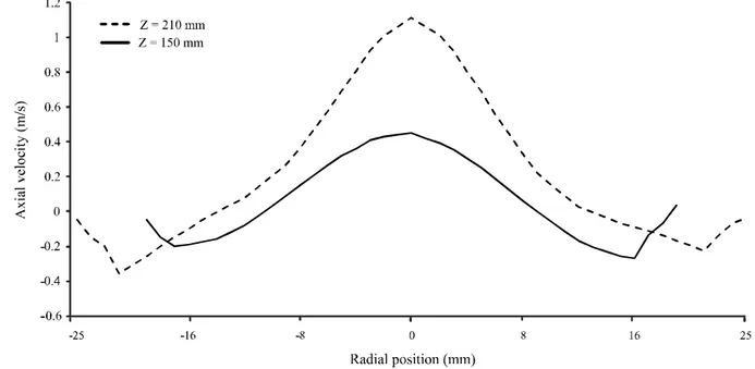
Figure 6 - Axial velocity profile along the radial position at different heights
Type of fluid Water Solid (soil)
Specific weight 997 kg m-3 2650 kg m-3
Dynamic viscosity 8,899 x 10-4 kg m-1s-1 8,899 x 10-4 kg m-1s-1
Volume fraction 98,32% 1.68%
Diameter Continuous fluid 15 µm
Inlet flow Mass flow water Mass flow solids 0.322 kg s-10.00234 kg s-1
Diluent Pressure 101 kPa
Concentrate Pressure 101 kPa
Walls (water) Non-slip
-Walls (solid) Slip free
-Experimental Simulated Error (%)
Delta P (kPa) 10 8.875 12.67
Mass flow at inlet - solids (kg s-1) 0.00234 0.00234 0.0
Mass flow of diluent - solids (kg s-1) 0.00174 0.00154 -12.98
Mass flow of concentrate - solids (kg s-1) 0.00088 0.0008 -10
Although not possible to compare to any experimental data, other observations can be made regarding the velocity profile within the hydrocyclone.
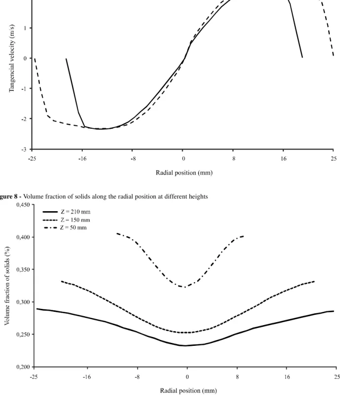
Figure 7 - Tangential velocity profile along the radial position at different heights
Figure 8 - Volume fraction of solids along the radial position at different heights
It can be noted from Figure 6 that the axial velocity is higher and positive along the central axis of the hydrocyclone, indicating an upward flow, and that with increasing radial position it decreases to zero at a distance of ± 13 mm. After that the axial velocities become negative indicating a downward flow, that is, the fluid moves in the direction of the outlet orifice of the concentrated suspension, reducing to zero near the wall of the hydrocyclone.
Figure 7 shows the tangential velocity profile of the water at two heights in the hydrocyclone, Z = 210 mm and Z = 150mm. The tangential velocity plays an important role in the performance of the hydrocyclone as it is of greater magnitude than the axial velocity, and produces the centrifugal force to separate the sediments. Figure 7 shows that the tangential velocity increases rapidly from the wall of the hydrocyclone to a maximum value at a radial position of ± 11 mm, indicating greatest centrifugal force.
In this case, when the sediments reach that position they will be thrown towards the wall of the hydrocyclone and continue in a downward flow to the concentrated suspension orifice, resulting in their separation. From the radial position of ± 11 mm to the centre of the hydrocyclone, the tangential force decreases until reaching a minimum value near the central axis. In that case, if a particle reaches this central area it will be carried in an upward stream out of the diluent suspension, meaning it will not separate from the water.
Figure 8 shows the volume fraction of solids along the radial position at three heights in the hydrocyclone, Z = 210 mm, Z = 150 mm and Z = 50 mm. It can be seen that the volume fraction of solids increases from the central axis of the hydrocyclone and reaches its maximum near the wall. This plainly shows the gradual accumulation of solid particles near the walls of the hydrocyclone. The maximum volume fraction of solids increases with a decrease in the y-coordinate. This observed change in the volume fraction of solids clearly demonstrates the process of separating solid particles from water in the hydrocyclone.
CONCLUSIONS
A computer model is used to simulate multiphase flow (liquid-solid) in a 50 mm hydrocyclone used in irrigated agriculture. The findings of this study lead to the following conclusions:
1. The RSM model is employed to describe anisotropic turbulence and the Eulerian model to simulate the presence of sediments. The applicability of this approach is confirmed by the good agreement between the simulated values and those obtained experimentally;
2. The field of axial and tangential velocities, the distribution of the static pressure and the volume fraction of sediments within the hydrocyclone are obtained. Knowledge of how these variables behave within the hydrocyclone makes CFD a useful tool in explaining the process of sediment separation in the hydrocyclone, while showing great potential in the optimisation of these devices.
REFERENCES
ANSYS® CFX - 13.0.Solver theory guide. 2010.
BRENNAN, M. CFD simulations of hydrocyclones with an air core: Comparison between large eddy simulations and a second moment closure.Chemical Engineering Research and Design,
v. 84, n. 6, p. 495-505, 2006.
CULLIVAN, J. C.; WILLIAMS, R. A.; CROSS, C. R. Understanding the hydrocyclone separator through computational fluid dynamics. Chemical Engineering, Research and Design, v. 81, n. 4, p. 455-466, 2003.
CULLIVAN, J. C.et al. New understanding of a hydrocyclone flow field and separation mechanism from computational fluid dynamics.Minerals Engineering, v. 17, n. 5, p. 651-660, 2004. DARMAWAN, U. R.; TADE, N.; LI, M.; EVANS, G. Hydrodynamic Simulation of Cyclone Separators. The Journal of the South African Institute of Mining and Metallurgy, v. 165, p. 501-548, 2011.
DYAKOWSKI, T.; WILLIAMS, R. A. Prediction of air-core size and shape in a hydrocyclone.International Journal Minerals Process, v. 43, n. 1/2, p. 1-14, 1995.
GRADY, S. A. et al. Prediction of flow field in 10-mm hydrocyclone using computational fluid dynamics. Fluid and Particle Separations Journal, v. 14, p. 1-11, 2002.
HSU, C. Y,; WU, S. J.; WU, R. M. Particles separation and tracks in a hydrocyclone. Tamkang Journal of Science and Engineering, v. 14, n. 1, p. 65-70, 2011.
MOTSAMAI, S. O. Investigation of influence of hydrocyclone geometric and flow parameters on its performance using CFD. Advances in Mechanical Engineering, v. 12, p. 12-22, 2010.
NARASIMHA, M.; BRENNAN, M.; HOLTHAM, P. N. Large eddy simulation of hydrocyclone prediction of air-core diameter and shape.International Journal of Mineral Processing, v. 80, n. 1, p. 1-14, 2006.
NOWAKOWSKI, A. F.; DYAKOWSKI, T. Investigation of swirling flow structure in hydrocyclones. Transactions of the Institution of Chemical Engineers, Chemical Engineering Research and Design, v. 81, n. 8, p. 862-873, 2003.
NOWAKOWSKI, A. F. et al.. Application of CFD to modelling of the flow in hydrocyclones. Is this a realizable option or still a research challenge?.Minerals Engineering,
SCHUETZ, S.et al. Investigations on the flow and separation behavior of hydrocyclones using computational fluid dynamics.
International Journal of Mineral Processing, v. 73, n. 2/4, p. 229-237, 2004.
SHOJAEEFARD, M. H.; NOORPOOR, A. R.; HABIBIAN, M. Particle size effects on hydrocyclone performance.
International Journal of engineering science, v. 17, n. 3/4, p. 9-19, 2009.
SOCCOL, O. J. Hydrocyclone for pre-filtering of irrigation water.Scientia Agricola, v. 61, n. 2, p. 134-140, 2004.
SVAROVSKY, L.Hydrocyclones. 2. ed. Lancaster:Technomic Publishing Inc., 1984. 354 p.
VERSTEEG, H. K.; MALALASEKERA, W.An introduction to Computational Fluid Dynamics: The Finite Volume Method. 2. ed. Prentice Hall, 1995. 267 p.
WANG, B.; YU, A. B. Numerical study of particle - Fluid flow in hydrocyclones with different body dimensions. Minerals Engineering, v. 19, n. 10, p. 1022-1033, 2006.
WANG, B.; CHU, K. W.; YU, A. B. Numerical study of particle - Fluid flow in hydrocyclone. Industrial & Engineering Chemistry Research, v. 46, p. 4695-4705, 2007.
ZHANG, J.; YOU, X.; NIU. Z. Numerical simulation of solid-liquid flow in hydrocyclone.Chemical Biochemical,