A Work Project presented as part of the requirements for the Award of a Master’s Degree in Finance from the NOVA - School of Business and Economics.
AN ANALYSIS OF LONG HORIZON EXCHANGE RATE PREDICTABILITY
Patrícia Vicente Lopes da Silva Santos, 25815
A Project carried out in the Master in Finance Program, under the supervision of:
Paulo M. M. Rodrigues
Abstract
Exchange rate predictability in long-horizons has turned into a debatable topic. Many were the ones achieving evidence of higher predictive power by economic models as larger periods were considered, while others argued against this premise. The main problem resides in the data properties that the regressors used exhibit, more specifically, overlapping observations, highly persistent regressors, and endogeneity, which affect the statistical inference. Consequently, if the biases are wrongfully corrected, invalid conclusions will be reached. Bearing this in mind, this analysis applies suitable tests aimed at overcoming these issues, after which it is inferred that mean-based regressions present weak statistical evidence on larger predictability in longer horizons. Lastly, a quantile regression is implemented, contemplating all potential biases. This innovative procedure finally provides results favoring long-horizon predictability.
Keywords: Predictability, Exchange Rates, Quantile Regression JEL Classification:E170, C530, F31
This work used infrastructure and resources funded by Fundação para a Ciência e a Tecnologia (UID/ECO/00124/2013, UID/ECO/00124/2019 and Social Sciences DataLab, Project 22209), POR Lisboa (LISBOA-01-0145-FEDER-007722 and Social Sciences DataLab, Project 22209) and POR Norte (Social Sciences DataLab, Project 22209).
I. Introduction
The foreign exchange market, widely known as the Forex market, is the over-the-counter market in which not only investors but also standard citizens, trade one currency for another for a large range of reasons, from standard tourism to investment trading. Being the largest trading market in the world in terms of volume, and also the most liquid one, many are the traders which rely on this market as to hedge against interest rate risk, or even speculate on geopolitical phenomena. The Forex market, as it is known today, was the result of the fall of the Bretton Woods agreement, in which most currencies were finally able to float freely, and, therefore, become a potential subject of predictability models as to possibly create trading opportunities. These investment strategies can be accomplished through the spot market, the forwards or the futures markets. As there has been strong evidence on weak short-run predictability of exchange rates, this analysis focuses on long-horizon predictability, which can be valuable in futures and forwards markets that bet on future values of the exchange rate.
Even though much of the currency price is set by demand and supply, another indirect driver in this process regards the central bank of the respective currency, whose main goal is to reduce the exchange rate volatility present in the market, as to lead to a more stable financial flow and economic growth. This is based on the implicit relationship between the exchange rate and the money supply, controlled through the interest rate. For instance, if, by chance, there is a need to depreciate the currency, then an increase in the money supply will do so. It produces an interest rate decrement that will enhance the exchange rate. Considering the variables taken as relevant in exchange rate analysis by investors, and the role that the central banks may play in the change in the price of the currencies, an analysis was developed aimed at predicting the return of the exchange rates in long-horizons. This way, the change in the exchange rate was regarded as the dependent variable, which, thereafter, was regressed on three predictors that concerned all factors above referenced: the industrial production (IP), the money stock (M1) and the WTI (West Texas Index).
The main drawback linked to this predictability procedure is associated with the data properties of the variables set as independent. In fact, as latter literature concludes, most of these regres-sions present serial correlation in the errors due to overlapping observations, endogeneity and high persistence in the process, which produce biases in the inferences. When these biases are wrong-fully corrected, researchers may be led to invalid conclusions on the evidence of predictability in long-horizons. This analysis is innovative in the way that it applies a new filtering procedure, the IVX, which is capable of overcoming all biases produced by the data properties already considered. Thereafter, a quantile regression was considered, through which it is concluded that there is, in fact, evidence of long-horizon predictability in exchange rates, especially in the extreme quantiles. Ad-ditionally, even though developed economies have a lower degree of predictability, these present a better performance at longer horizons, which contrast with the developing countries that present larger predictive power, although it is more focused in shorter-horizons.
This analysis is organized as follows. Section II comprises the literature linked to the topic, which motivates this research. Section III considers all the data required to proceed, as well as the economies subject to this empirical analysis. In Section IV, all methodology is presented, from the most simple model, that does not account for all biases, to the quantile regression method, which considers all potential biases. Section V presents the results, which are capable of corrob-orating the premises defended in previous literature as discussed in Section II. Finally, Section VI sums up the results and concludes.
II. Literature Review
For many years exchange rate predictability was a subject of research with no significant results. Meese and Rogoff (1983), for example, provided a monthly post-sample fit analysis for different ex-change rates. Years later, in Meese and Rogoff (1988), ex-changes in the exex-change rate were regressed on real interest rate differentials in order to predict the real dollar/Deutsche mark exchange rate. Finally, Engle and Hamilton (1990) exploited non-linearities in the exchange rate, while Diebold and Nason (1990) resorted to non-parametric estimates of the conditional mean weekly percentage
change in the nominal exchange rate. In all cases, the random walk with and/or without a drift outperformed the more sophisticated approaches. The random walk and standard economic model
comparison, also known as the Meese-Rogoff puzzle 1, was further evaluated in Rossi (2005),
where the properties of the variables were regarded as the source of the apparent unpredictabil-ity in the economic regressions. As these characteristics were taken into account, the forecasting superiority of the random walk was shown to not be as significant as previously inferred.
Mark (1995) encountered statistical evidence on exchange rate predictability, in the quarterly rates between the U.S. dollar, the Canadian dollar, the Deutsche mark, the Swiss franc and the Japanese yen from 1973 to 1991. Assuming the purchasing-power-parity and uncovered-interest-parity hold, the model regressed the change in the exchange rate on the difference between the fundamental value of the exchange rate, that is, the result of a monetary model where the exchange rate is moved by a linear combination of the log relative money stock and the log relative real income, and its spot rate. From the experiment, it was inferred that the model performed better than the random walk and that it displayed increasing predictive power. In fact, not only the regression produced lower Root-Mean-Squared-Errors than the benchmark model (the random walk), but this difference also became larger as longer horizons were considered. Additionally, the coefficients, the t-statistics and the R2were also achieving higher values when the prediction horizons increased.
The diversity of the results is a direct consequence of the data issues that the analysis aimed to overcome, as well as the method that they used to achieve so. To begin with, the strong persistence present in the regressors will be considered, which leads the coefficients to be biased away from zero and the distribution skewed to the right. On the one hand, Mark (1995) carried out a Monte Carlo simulation where inference was drawn from Gaussian and non-parametric bootstrap distribu-tions, under the null of no predictability in log exchange rates and assuming co-integration between the fundamental and the spot rate. On the other hand, according to Rossi (2005), the variables are not only highly persistent, but these also present evidence of a not fully co-integrated process. This 1The Meese-Rogoff puzzle is the process in which exchange rate models cannot outperform the random walk in out-of-sample forecasting of exchange rates. The origin of the puzzle goes back to the 1983 Meese and Rogoff paper.
is crucial for the procedure in hand, as the closer the root is to unity, the more the estimated error conflicts the economic model’s estimation when compared to the random walk. The effect pro-duced by these two data characteristics may have biased the results achieved by researches that did not account for these properties.
Rossi (2005) proposed a test for equal predictive ability between the random walk and the Meese-Rogoff models, which was robust to high persistence. It considered a local-to-unity variable and when applied to the puzzle, the random walk was found to perform better at forecasting, even though the resulting improvements were not regarded as statistically significant at all horizons and all currencies. In Berkowitz and Giorgianni (2001), two different simulations were performed. In the first, critical values were computed through Monte Carlo simulations under the assumption of no co-integration, that is, the exchange rates were assumed to be independent of economic fundamentals. In the second, an unrestricted bivariate VAR was fitted to generate the critical values, in which the co-integration assumption was relaxed and an exact unit root was assumed. The critical values of the first experiment were lower than those from the second simulation but higher than the ones obtained by Mark (1995), only encountering evidence of predictability for the U.S. dollar/Swiss franc exchange rate. In conclusion, inference depends on the assumptions and if there is no co-integration and its existence is assumed, then the regression may come close to a spurious regression.
Secondly, this research resorts to variables that are endogenous and, therefore, create a significant bias in the estimated coefficients. Hjalmarsson (2011) developed a new econometric method that relies on a simple modification of the regression. The residuals resulting from an AR(1) of the regressor are used as an explanatory variable in the main regression. In the end, the final regression does not present evidence of endogeneity and the results are affected: when there is no adjustment and the standard Newey-West standard errors are used, it is concluded that predictability increases with longer horizons; when applying the modification and scaling the t-statistic by the prediction horizon, there is evidence of a reduction in predictability. Hjalmarsson also investigated the power
properties of the statistic and observed that its predictive power decreased as the horizon increased. Lastly, the existence of overlapping observations, due to the aggregation of the dependent variable at longer horizons, also influences the results. It creates serial correlation in the regression errors (Moving Average (MA) behavior) which, in turn, leads to wrong inferences. To overcome this problem, Mark (1995) provided a Covariance-Matrix estimator robust to serial correlation in the errors.
For the purpose of exchange rate predictability, a Quantile Regression Model was also applied. Recently, these models have become one important tool in many areas of research because of its out of sample performance and ability to provide a complete picture of the statistical relationships. For instance, Taylor (2007) applied an exponentially weighted quantile regression to forecast daily supermarket sales, which outperformed the conventional mean regression. Additionally, Bulligan et al. (2017) resorted to quantile regressions on the inflation rate, in which a better description and superior forecast of the conditional distribution of the inflation rate was achieved. In fact, the variable’s distribution presented variations throughout time, which could not be captured by the benchmark model. Finally, quantile forecasts of volatilities have become increasingly important due to new emerging products based on the volatility index. Park et al. (2017) achieved a new parametric quantile forecast which produced improved predictability of the forecast intervals of volatilities.
Koenker and Basset (1978) were the first to introduce the conditional quantile regression models, as a way to better respond to cases in which the impact of a given regressor will depend on the outcome level of the response variable. That is, in situations where there is a need to achieve a model in which the estimator distribution would change according to the parametric class of the distribution of the regressand. It is important to note that, even though quantile models seem to have better outcomes, these may not be the most suitable procedures. There may exist variables whose data characteristics are not fit for quantile estimation. In these specific cases, the mean regression will correspond to the most suitable tool. In conclusion, there was an increasing need to create
methods that could identify cases in which quantile models would be the best approach.
In order to analytically identify variables that are predictable through quantile regressions, the
Quantile Information Criterion (QIC) was introduced. Huarng and Yu (2014) applied the
coeffi-cient of variation as the information criterion - the ratio of the standard deviation and the mean of the variable - in order to measure the dispersion of the variable’s distribution. According to Huarng et al. (2014), variables with large variations tend to be difficult to predict. Aiming to achieve a method that could determine which variables could be, in fact, predicted, Huarng and Yu (2014) accomplished thresholds on the coefficient of variation: if the coefficient lied outside the thresh-olds’ range, the variable could not be forecasted; otherwise it would be possible to predict. So that the thresholds could be computed, two different and independent data sets were used: a sample data set and a target data set. The sample data determined the thresholds for the QIC which would, thereafter, understand if the variable in the target data set could be predicted. In the end, the ef-fectiveness of this criterion was evaluated by comparing its results to the criterion developed by Huarng et al. (2014). In this case, there was evidence of an increased forecasting performance.
III. The Data
Monthly data was obtained from the Federal Reserve Bank of St.Louis. This data includes the United States and other economies with which the dollar is priced against. These countries were grouped into two distinct sections according to their economic, financial and geographical charac-teristics: developed economies and developing economies. Regarding the Developed Economies, these are the Euro Area, as a monetary union; the United Kingdom, a European country which has never participated in monetary arrangements; Japan, which is representative of the Asian economies and, finally, Canada, that establishes close ties with the United States. In terms of the Develop-ing Economies, these were chosen dependDevelop-ing on their different geographical and cultural aspects: Brazil, Mexico, India, Poland, and Turkey. These represent Latin and Central America, South Asia, Western Europe, and Western Asia, respectively. It is important to highlight that all economies con-sidered have a floating type of exchange rate regime, as these are the only ones that can be subject
to this sort of analysis.
In the model construed, the influence that productivity, money stock, and the oil prices have on the exchange rate is being analyzed. In order to measure productivity, the Industrial Production In-dex was used instead of the Gross Domestic Product, since the latter is only available at a quarterly frequency and the present analysis uses monthly data. In terms of the money stock, the M1 was ex-tracted, being given by the currency plus checkable deposits. Finally, the influence of the oil prices on the exchange rate was also explored through the West Texas Index (WTI). This variable not only aims to determine the impact of the oil prices on the subject of analysis but also represent the macroeconomic conditions of the distinct periods that may have had an influence on the exchange rates. The periods evaluated for each country varied according to data availability.
IV. Methodology
The first stage of this research will focus on the impact of the level of industrial production, the money stock and oil prices at a given period t, on the change of the logarithm of the exchange rate between the United States’ dollar and the other economies’ currency, h periods ahead. Considering the data available for each distinct economy, the change of the logarithm of the exchange rate (∆et+h) was regressed on the respective industrial production index (yt), the money stock (mt) of
the economy and on the WTI (oilt), for 12-, 24- and 36-months a-head. The first difference was
imposed as to consider the returns of the exchange rate as the dependent variable of the regression. Taking this into account, the regression is given by:
∆et+h= c + β1yt+ β2mt+ β3oilt+ ut+h (1)
The estimation of the model presented in (1) was submitted to different procedures so that the problematic data properties could be taken into account, that is, the overlapping observations, high persistence and endogeneity. In fact, these will affect the validity of the results. The first issue to be
tackled involved the computation of the Newey-West (NW) and the Hansen-Hodrick (HH) standard errors, which aimed to overcome the bias created by serial correlation in the errors. Although these new methods also attempt to consider the other two potential problems (strong persistence and endogeneity), these do not accomplish the expected results. In fact, Kostakis et al. (2018) were capable of demonstrating an over-rejecting of the null when highly persistent variables were employed as predictors with these types of standard errors. They concluded that the presence of overlapping observations in long-horizon predictive regressions impacts the empirical size of the t-test with the NW and HH standard errors and, consequently, the power to reject the null is also affected. As the predictive horizon increases, the statistics become even more oversized and, in the end, it may even lead to a spurious regression.
The biases produced by endogeneity and high persistence will now be considered, not only because these properties tend to be common in the variables under analysis, but also due to the invalid statistical inference these may produce. The procedures that will be further discussed are based on Hjalmarsson (2011), in which the root of the AR(1) process was regarded as being a local-to-unity, drifting closer to unity as the sample size increases, that is, ρ = 1 + c/T . On the one hand, this method may be more flexible when compared to a pure unit-root. Nevertheless, it should still be regarded as restrictive, since the processes considered cannot be implemented on variables that are less persistent than the local-to-unity case. As to understand if the variables used follow this type of behavior, an AR(1) was estimated for each one of the regressors. Thereafter, two different methods were performed: one assumed the value of c to be known, another applied the Bonferroni method developed by Campbell and Yogo (2006) as to overcome the fact that c is difficult to estimate and, most of the times, unknown.
Regarding endogeneity, for each of the regressors considered, Hjalmarsson (2011) first suggests the computation of the correlation between the residuals from an AR(1) process and the residuals from a single-predictor regression. According to Hjalmarsson (2011), if the resulting correlation is different than zero, then it can be inferred that endogeneity is present in the process. Thereafter, a
simple modification to the regression is performed, where the dependent variable is regressed not only on the predictor that is being evaluated but also on the residuals that were computed from the AR(1) model above. Afterwards, under the null of no predictability and exogenous regressor, the test statistic is scaled, that is, it is divided by the square root of the horizon considered. This new robust statistic will follow a standard normal distribution. Even though this procedure may seem more successful at overcoming the present biases than the NW and the HH standard errors, when evaluating the size properties of this test, Hjalmarsson (2011) found that the scaled test statistic presented an over-rejection when upon endogenous variables with negative correlations. This is the reason why an alternative method was constructed, in which the assumption on the known c was dropped and Bonferroni methods were implemented. Taking this into account, a confidence interval for c through a unit-root test developed by Chen and Deo (2009) was computed, being based on a restricted likelihood approach.
This way, for each value of c achieved, the respective t-statistic was computed. Considering all possible values of the t-statistic, the most conservative values were extracted, more precisely, the maximum and the minimum t-statistic. Each one of the statistics were then used for comparison depending on the type of test. If, on the one hand, the null hypothesis of no predictability was tested against H1 : βq > 0, then the scaled minimum t-statistic was used. If, on the other hand, the
alternative hypothesis was given by H1 : βq < 0, the maximum scaled test statistic was applied. The
statistics were then compared to the critical values of the standard normal distribution. According to Xu (2017), the scaling performed by Hjalmarsson (2011) in local-to-unity cases tends to over-estimate the standard error if the predictor ends up being just weakly dependent. Additionally, under the null hypothesis of no predictability, when resorting to the asymptotics allowing for long horizons and several levels of persistence, Xu concluded that the scaled t-statistic of Hjalmarsson (2011) converged to zero if h(1−ρ) → ∞, where ρ is the parameter of the AR(1) and h the forecast horizon. This way, if the predictor is not as highly persistent, even if there is statistical evidence of predictability in the first periods, the significance will disappear as longer horizons are considered.
In order to overcome this insignificance in longer horizons, Xu resorted to an implied test in which the implications of the short-run predictability model were tested using Bootstrap critical values. As to introduce the different levels of persistence that the regressors may present, the parameter
of the AR(1) process was established as being ρ = 1 + cn−r, where c only takes non-positive
values, and r accomplishes the different levels of persistence. A similar implied test presented by Rossi (2007) was conducted, nevertheless, it only concerned the local-to-unity specification. In this situation, the method introduced by Xu is more suitable, as it allows for different levels of persistence. In this experiment, the asymptotic distribution of the implied test is computed not only for the predictability hypothesis but also for the non-predictability hypothesis, controlling for the size under the various degree of persistence. The test developed has shown that its predictive power does not vanish as longer prediction horizons are regarded, independently of the level of persistence, which corresponded to a drawback in the process developed by Hjalmarsson (2011). Additionally, not only the test was shown to be more powerful than the scaled test of Hjalmarsson, but there were also conducted simulations that corroborated the premises of a significant power gain of the implied test over other widely-used tests. The predictability of the rates was tested through the implied test, which was compared against one-sided and two-sided Bootstrap critical values at the 5% level.
Besides the scaled OLS-regression, the Hjalmarsson and Xu methods, there is another approach aimed at solving potential biases created by high persistence, the Extensive Instrumental Variable (IVX) approach. If in the procedures performed above there was a certain rigidity on the type of roots that the regressors may present, this new test will provide a higher level of flexibility. This new process consists of constructing an instrumental variable that explicitly controls the degree of persistence of the variable and, this way, account for very general time series characteristics: from pure stationary to pure non-stationary processes, including all other intermediate persistence pos-sibilities. This feature is considered to be an advantage, as it can be implemented on any variable, independently of its time-series properties. Moreover, the test statistic accomplished presents good finite-sample properties, allowing for valid inference: the estimator follows a normal distribution
and the test statistics a chi-squared distribution under the null. Finally, whereas all different proce-dures above, which only rely on univariate models, the IVX is applicable for multivariate predictive regression systems.
As to avoid potential biases in the inference created by strong persistence and endogeneity in the macroeconomic variables taken into account, a final method was introduced, the IVX-QR devel-oped by Lee (2016). This is an association of the quantile regressions with the most suitable procedure in overcoming the biases. In fact, one common issue between the mean regressions and the quantile-type approach resides in its biasedness in inferences produced by variables with these kinds of properties. Additionally, according to the limit theory of ordinary QR with persistent re-gressors, the distortions produced become even larger as predictors with stronger endogeneity, high degrees of persistence and extreme quantiles associated with fat-tails are regarded. According to Lee (2016), the distortions produced by these data properties can be represented by a non-standard inference given by λ(τ ) ∗ ηLU R(c).The λ(τ ) is the sum of a linear dependence effect and the
trun-cated mean of regressions errors that, in the end, accounts for the endogeneity that is set to be removed in order to have valid inferences in a QR. This parameter can also be computed through −corr[(1(u0tτ < 0), uxt]. On the other hand, ηLU R(c) represents the non-stationary distortion,
being a local unit root t-statistic. As to overcome this problem, an IVX filtering method was con-sidered, where most of the discriminatory power is kept unchanged. This way, after the quantile regression is estimated, a valid inference can be formed alongside suitable size properties, in which the estimator will follow an asymptotic mixed normal distribution. Taking this into account, the regression will be represented in the following way:
∆et+h= β0+ β 0
1xt+ ut+h (2)
xt+h= Rnxt+ ux(t+h) (3)
Rnis the component that introduces the persistence flexibility, being given by Rn = IK + C/nα,
which can be categorized as follows.
• I0 - Stationary: α = 0 and |1 + ci| < 1, ∀i
• M I - Midly Integrated: α ∈ (0, 1) and ci ∈ (−∞, 0), ∀i
• I1 - Local to Unity and Unit Root: α = 1 and ci ∈ (−∞, ∞), ∀i
• M E - Mildly Explosive: α ∈ (0, 1) and ci ∈ (0, ∞), ∀i
As in the IVX, one of the main advantages of this procedure relies on the possible implementation of this method to a large range of persistent variables, from the stationary to the lightly explosive predictor. Independently of the degree of persistence in the regressor, the goal of the IVX-QR is to create an instrumental variable of intermediate persistence by filtering a persistent and potentially endogenous predictor. In the end, considering the different categories of persistence, if the regressor is I0 or M I, the original level of persistence is kept, whereas cases in which the predictor is I1 or M E. For the first, it is turned into a M I process, while the second becomes similar to an OLS for mean regression cases.
As previously stated, the distortion produced by the variables in the analysis is calculated through λ(τ ) ∗ ηLU R(c). So that the biases created could be corrected, two different procedures could be
implemented. One is very similar to the Hjalmarsson (2011), in which the size distortion is tackled through an induced confidence interval of the estimator by computing another confidence interval for c. Even though it is capable of achieving the correct size, this Bonferroni method is only valid for local-to-unity cases and, therefore, cannot be considered for variables with lower persistence. Another, that is suitable for this analysis, is the IVX filtering technique. It intents to filter persistent regressors (xt) to generate zt, at the same time that local power does not suffer any significant
changes and a proper size correction is achieved. ztdepends on a filtering coefficient, F , and a first
difference operator:
zt = F zt−h+ ∆x (h)
This equation leads to a range of results that go from the setting of the first difference to a level data with no need for filtering. In fact, if F = 0k, then zt = ∆x(h)t . This first difference is
implemented in many cases, however, even though the standard normal or chi-square distribution are achieved, there is a reduction in the convergence rate linked to lower local power. Conversely, when F = Ik, then zt = xt, where a size distortion is associated with an unchanged statistical
power and convergence rate. Finally, for this particular case, the filtering element will be given by the auto-regressive component in the IVX, Rnz, which is determined by Ik+Cz/nδ = 1+c(δ, n)/n,
with c(δ, n) = n1−δcz. This way, δ ∈ (0, 1) and cz is negative. The IVX superiority comes from
the exploitation of the advantages from resorting to a level and a first difference. In fact, the discriminatory power, from the first, and the size correction, from the second are accounted for in the filtering. Taking this into account, it is now necessary to determine the values of (Cz, δ)
to construe the IVX. This is such that the standard normal limit theory for the t-statistic of the parameter will hold for any δ ∈ (0, 1) as the sample size increases, that is, n → ∞. The c(δ, n) → −∞, leading ηLU R(c) to converge to a standard normal distribution.
Bearing this in mind, it is inferred that, for a specific finite value of n, the chosen value of |n1−δcz|
has to be large enough for the standard normal limit theory of tβ1,τ to hold. Lee (2016) defends
that δ should be large enough to not compromise the local power, but needs to be small enough so that the standard normal distribution can be accomplished, as lower δ are able to better correct size distortions. So that this puzzle could be overcome when assuming a finite sample for a local unity regressor, a value for δ ∈ (0, 1) was chosen with a normalized cz that controls the size distortion
even after considering a tolerated Type I error bound. Lee (2016) tabulated the values of c(δ, n) and λ(τ ) that, for a 5% test level, have suitable tail approximations. Depending on the value of λ(τ ), which is easily computed through the residuals, as previously shown, the c(δ, n) is picked. In the analysis performed by Lee (2016), the value chosen for cz was −5 and, after normalizing this
value and picking a fitted value for c(δ, n), the δ could finally be computed through the following expression: δ = 1 − [log(−c(δ, n)) − log(5)]/log(n). This way, only λ(τ ) is estimated. This is an advantage, as choosing a specific value for czavoids certain invalid problems with I0 − M I.
Now that all parameters needed to perform the IVX-QR are all computed, its estimation and tests can be accomplished. Taking this into account, the first step comprises the estimation of the IVX-QR with dequantiling, that is, through ytτ = β
0
1,τxt−h + u01tτ, where ytτ = yt − β0,τQR(τ ) as to
achieve a zero-intercept quantile regression. β0,τQR(τ ) corresponds to the coefficients resulting from the quantile regression with intercept. Thereafter, so that the t-statistic can be computed, the only component that is missing is the standard error of the coefficient, which is calculated through the usual standard error formula for quantile regressions. It requires the distribution of the residuals, more precisely, the density at that given quantile. Nevertheless, it is known that, after all biases considered, it will follow a normal distribution.
V. Results
In the first stage of this analysis, the change in the logarithm of the exchange rate k periods a-head (∆et+k) was regressed on the Industrial Production (yt), M1 (mt) and the oil prices (oilt). This
re-gression was robust to the serial correlation in the errors produced by the overlapping observations through the implementation of the Newey-West and Hansen-Hodrick standard errors2. In order to
determine if there is statistical evidence favoring a higher predictive power in larger horizons, the increasing or decreasing behavior of the t-statistics was observed. If there was an enhancement of the absolute value of the statistic towards the critical value that would provide statistical sig-nificance, then it would be inferred that there would exist enough evidence that could satisfy the premise of a higher predictability in longer horizons. Otherwise, the opposite would be concluded. Additionally, as defended in past literature, the performance of the coefficients, the R2and the Ad-justed R2 was also considered as a parameter, in such a way that an existent positive relationship
between these values and the horizons would mean an increasing ability to forecast the exchange rates. An example of the analysis performed is shown in figure 1, where the different statistics for the Euro Area and India are evaluated through the different horizons.
Regarding the developed economies3, there is an overall positive correlation between the t-statistics
of the distinct variables and the horizons. For the Industrial Production in the NW, only the United Kingdom has no positive correlation between the horizons and the t-statistic, leading to an inability to reject the null. The same is observed in the HH, with the exception that Japan is unable to accomplish significance. Regarding the M1, all economies have an increasing behavior of the absolute statistic in the NW, however, only Canada and the Euro Area are capable of achieving a rejection of the null. In the HH case, only the Euro Area stands outside the critical value interval. Finally, for the WTI, only the United Kingdom and the Euro Area have an increasing absolute t-statistic, moving in the same direction as the critical value of statistical significance. In the end, only these two economies are able to achieve significant coefficients. In fact, Japan and Canada have their statistics exhibiting behavior in the opposite direction of the critical values, and, consequently, these are not able to accomplish significance. The only difference to the HH is that the United Kingdom is incapable of having significant coefficients.
Concerning the coefficients, it is also verified that the longer the horizon, the higher the absolute value of the coefficients: the positive coefficients become even more positive and the negative coefficients achieve even more negative values. This occurs for all variables and for every horizon for economies such as the Euro Area and Canada. Japan and the United Kingdom have a similar trend for all cases, except for one and two situations, respectively. Regarding the goodness-of-fit measures, all present increasing trends as the horizons become larger, except for Japan, whose values decrease from the first to the second period considered. Lastly, it ought to be highlighted that the HH standard errors may follow the same trend as the NW, but these tend to have a lower rejecting power over the null than the latter. In fact, all statistically significant cases in the HH are also significant in the NW case, but there were situations in which the HH type of standard error would not reject the null, while the NW was capable of achieving so. This behavior is also extendable to the developing economies, as it will be shown below.
Moving on to the developing economies4, the t-statistic behavior tends to be diverse. If, on the one
hand, Turkey has all statistics favoring a larger predictive power linked to significant coefficients, on the other hand, Brazil only has M1 with a positive relationship between the horizons and the t-statistics, even though it is not capable of achieving significance for both NW and HH. The same pattern is observed for India and for Mexico, which have predictive evidence in the Industrial Production and the WTI, respectively, although significance is not accomplished for the HH case. In terms of the change in the coefficients throughout the horizons4, an increase in absolute value for all
variables and all horizons for economies such as Turkey and Mexico is observed. Poland has only reducing coefficients for larger horizons for yt, while India and Brazil present the same decreasing
behavior for oilt. Concerning the goodness-of-fit measures, all economies verify a positive trend
between the measures and the larger horizons, except for India, whose values decrease from the 24-month to the 36-month horizon.
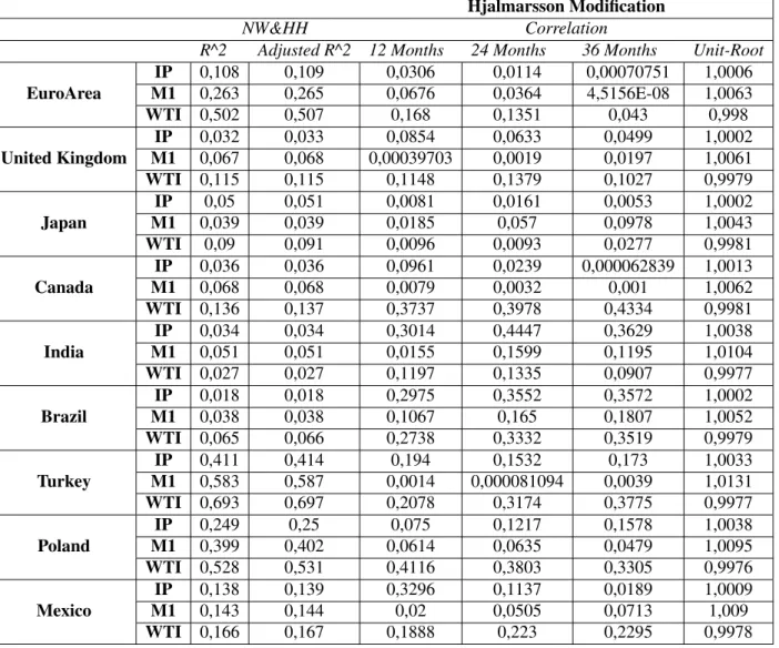
Now that the robust standard errors through the NW and HH methods were considered, the results on the Hjalmarsson will be stressed , which aimed to better repress the biases created by endoge-nous and persistent variables in cases of overlapping observations. In terms of the presence of a unit-root 5, all countries analyzed had a root close to unity, independently of being regarded as a developed or developing economy. Thus, it can be inferred that the Hjalmarsson methods, which could only be applied to local-to-unity cases, can be resorted to the sample in analysis. Next, so that the Hjalmarsson method could be performed, the correlation between the residuals of the AR(1) and the OLS regression on each regressor was computed5. It should be noted that the developing economies tended to reach higher values of correlations than the developed economies, although the values achieved were considered to be low for most of the cases.
The Hjalmarsson statistic was thereafter computed 6. When performing the predictability
anal-ysis of before and comparing these results with the ones from the NW and HH standard errors, 4Figure 3 to 6 and Table 3 to 6 - Annex
5Table 6 - Annex
an abrupt change in the number of cases in which a higher predictive power for longer horizons is linked to significance is observed. In fact, all developed economies have evidence against the presence of exchange rate predictability, except for the Euro Area which has an increasing absolute t-statistic growing towards the critical value, accomplishing significance afterwards. When com-paring the developed economies with the developing ones, it is clear that, for a 95% confidence interval, the latter ones have a higher rate of rejection of the null. In fact, Brazil has the exact opposite behavior of the developed economies: all variables present values favoring the exchange rate forecasting premise. Conversely, India has the same pattern as the developed economies and the remaining developing cases do not present higher predictive power, even though these exhibit significant coefficients. Mexico, however, only has significance in the Industrial Production.
In conclusion, as this procedure accounts for endogeneity and persistence, there is an under-rejection of the null, which may imply biases in the NW and the HH results. Moreover, it is also observed that developing economies tend to reject more the null than the developed economies. Regarding the Bonferroni method7, the Euro Area, Japan and Brazil have evidence against signif-icance upon the minimum statistic. It tends to move in the opposite direction of the critical value that provides significance, as larger horizons are considered. The remaining economies, although these have evidence of a growing predictive power, it is not sufficient to accomplish significance. Conversely, the maximum threshold on the Bonferroni has all developing economies, with the ex-ception of Brazil, exhibiting evidence against long-horizon predictability. The statistic varies in the opposite direction of the maximum critical value. In the developed economies, however, there is behavior favoring higher predictive power, even though significance could not be achieved.
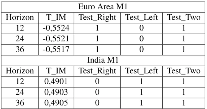
Aside from the Hjalmarsson case, the implied test by Xu 8 was also performed as to achieve a
higher degree of flexibility in the inference. In terms of the change of the statistics across larger predictive horizons, it is clear the change is not very significant, as it can be observed in Table 1
7Table 3 to 5 - Annex 8Tables 7 and 8 - Annex
Euro Area M1
Horizon T_IM Test_Right Test_Left Test_Two
12 -0,5524 1 0 1
24 -0,5521 1 0 1
36 -0,5517 1 0 1
India M1
Horizon T_IM Test_Right Test_Left Test_Two
12 0,4901 0 1 1
24 0,4903 0 1 1
36 0,4905 0 1 1
Table 1: Implied Test of Xu example: Euro Area and India M1
9. In fact, there are situations in which the implied test does not change throughout the different
periods considered, as it is the case of the United Kingdom and Brazil for the Industrial Production and M1, respectively. The significance of the statistics against the right-sided, left-sided and two-sided Bootstrap critical values for a 5% significance level will then be evaluated. Important to note that, as it will be verified, this method tends to have more situations in which there is significance, when compared to the Hjalmarsson test.
Considering the different variables, the Industrial Production has no significance for all developed economies, except for Canada, which reaches values above all critical values for the 36-month horizon. Regarding the developing economies, India and Brazil have no cases of significance, whereas Turkey and Mexico, which achieve significant tests for the right-sided and two-sided tests for the 24- and month horizon. Poland has a similar behavior, but aside from the 24- and 36-month horizon, the 12-36-month horizon is also significant. Concerning the WTI, only Turkey has all horizons significant for the left and two-sided test, while Poland has the 12- and 24-month left test significant. All other economies have no cases of significance. Finally, for the M1 the results are diverse. If, on the one hand, Brazil has no cases of significance, on the other hand, Turkey and the Euro Area have all horizons significant for the right and two-sided tests, while India has all left and two-sided tests above the critical value. All in all, all other situations have the 24- and 36-month horizon significant for the left/right sided test, along with the two-sided one. It can be inferred that
there is a higher tendency for the implied test to have a significant coefficient for longer horizons than for shorter ones.
The IVX was, thereafter, computed, accomplishing the highest level of flexibility when it comes to the degree of persistence of the regressor 10. An overall observation of the results leads to the
conclusion that, through the imposition of the IVX, there is a large decrease in the variation of the t-statistic throughout the different horizons when compared to the procedures performed before. For example, the Euro Area has an almost constant statistic for the Industrial Production and the WTI, as well as the United Kingdom, whose values suffer a very short variation when considering longer horizons. Additionally, there is a sudden reduction in the ability to reject the null of no predictability. For instance, in the developed economies, only the Euro Area in the M1 is capable of achieving increasing absolute t-statistics, converging towards the critical value and accomplishing significant coefficients. All the other cases have their statistics stand inside the confidence interval, presenting a very low variation between horizons. Regarding the developing economies, almost all of them have the same behavior as the developed ones, except for Mexico and Turkey, whose statistics have a relevant decrease in value, going in the opposite direction of statistical significance. The predictive power decreases with larger horizons, to the point where Turkey started out with significant coefficients and, at longer horizons, these ended up being insignificant.
Figure 1: Industrial Production of the Euro Area and India (developed and developing economies)
From the results above, it is concluded that, through the IVX, the economies tend to present little evidence of statistical predictive power in exchange rate forecasting. Thus, when accounting for all biases produced by the issues discussed above in a standard mean-regression, the independent variable under analysis ends up achieving a low degree of potential predictability. Since this last procedure corresponds to the one that best accounts the data problems in hand, it was thereafter considered for the quantile regression application11. The empirical results of the IVX quantile
re-gression on exchange rate predictability will then be examined. First of all, this analysis comprised single and multiple-predictor regressions for horizons already studied in the procedures above (12-, 24- and 36-months) and for quantiles that ranged from the 10% to the 90% with a 10% step. The single variable regressions were computed as to more easily compare them with the cases in which it was only possible to achieve single predictor regressions. Thereafter, the multiple predic-tor quantile regression was accomplished to fully take advantage of the properties of the IVX-QR, more specifically, the possibility to regress the dependent variable in more than one regressor. Fi-nally, it was also possible to compare the results between the single and multiple variable quantile regressions in terms of predictive power. An overall view of the empirical results of this method can clearly infer that the regressions with a single variable still have difficulty on achieving signif-icant coefficients, as in the methods previously analyzed, while the multiple predictor regression is capable of providing a more complete understanding of the potential predictive power of the predictors.
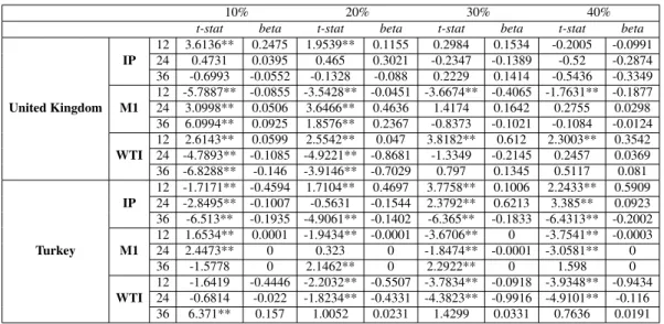
Focusing on the multiple-predictor regression, similarly to the results achieved by Lee (2016), there is a slight tendency for extreme quantiles to have t-statistics outside the confidence interval. Never-theless, this behavior is not as strong as in the case of Lee (2016). In fact, the developing economies have their significant cases uniformly distributed throughout the different quantiles, while the de-veloped economies have them more concentrated on quantiles ranging from the 10% to the 30% and from the 70% to the 90% quantile. This is consistent with the results previously discussed. Impor-tant to note that, once again, the developing economies present a higher predictive power than the
10% 20% 30% 40%
t-stat beta t-stat beta t-stat beta t-stat beta
United Kingdom IP 12 3.6136** 0.2475 1.9539** 0.1155 0.2984 0.1534 -0.2005 -0.0991 24 0.4731 0.0395 0.465 0.3021 -0.2347 -0.1389 -0.52 -0.2874 36 -0.6993 -0.0552 -0.1328 -0.088 0.2229 0.1414 -0.5436 -0.3349 M1 12 -5.7887** -0.0855 -3.5428** -0.0451 -3.6674** -0.4065 -1.7631** -0.1877 24 3.0998** 0.0506 3.6466** 0.4636 1.4174 0.1642 0.2755 0.0298 36 6.0994** 0.0925 1.8576** 0.2367 -0.8373 -0.1021 -0.1084 -0.0124 WTI 12 2.6143** 0.0599 2.5542** 0.047 3.8182** 0.612 2.3003** 0.3542 24 -4.7893** -0.1085 -4.9221** -0.8681 -1.3349 -0.2145 0.2457 0.0369 36 -6.8288** -0.146 -3.9146** -0.7029 0.797 0.1345 0.5117 0.081 Turkey IP 12 -1.7171** -0.4594 1.7104** 0.4697 3.7758** 0.1006 2.2433** 0.5909 24 -2.8495** -0.1007 -0.5631 -0.1544 2.3792** 0.6213 3.385** 0.0923 36 -6.513** -0.1935 -4.9061** -0.1402 -6.365** -0.1833 -6.4313** -0.2002 M1 12 1.6534** 0.0001 -1.9434** -0.0001 -3.6706** 0 -3.7541** -0.0003 24 2.4473** 0 0.323 0 -1.8474** -0.0001 -3.0581** 0 36 -1.5778 0 2.1462** 0 2.2922** 0 1.598 0 WTI 12 -1.6419 -0.4446 -2.2032** -0.5507 -3.7834** -0.0918 -3.9348** -0.9434 24 -0.6814 -0.022 -1.8234** -0.4331 -4.3823** -0.9916 -4.9101** -0.116 36 6.371** 0.157 1.0052 0.0231 1.4299 0.0331 0.7636 0.0191
Table 2: T-statistics from the Multiple IVX-QR - Euro Area and India (10% to 40% Quantile)
developed ones, which is observable through the comparison between Turkey, which has almost all coefficients significant, and the United Kingdom that finds some trouble in accomplishing statistics outside the critical value range, specially in the Industrial Production. This difference, however, is less predominant than in the procedures above, as the developed economies present a higher level of statistical significance - Table 2. Additionally, when comparing the predictive power between the variables in hand, it is verified that the Industrial Production and M1 accomplish significance more frequently than the WTI. Finally, it ought to be referred that, for the economies with the highest number of significant coefficients, the horizons that have the strongest evidence of predictability are the longer ones, as it occurs with the developing countries. Conversely, the countries with the lowest number of significant coefficients have their shorter horizons presenting higher evidence of exchange rate predictability.
VI. Conclusion
This paper explores different methods of exchange rate predictability, which aim to control all bi-ases created by common data properties in the regressors used, such as serial correlation in the errors produced by overlapping observations, strong persistence and endogeneity. The first method focused on the first issue through the imposition of NW and HH standard errors, concluding that, even though not most of the economies have statistical evidence favoring a higher predictive power
when considering larger horizons, it corresponded to the procedure that was able to achieve the highest number of statistically significant prediction cases. The only problem associated with the NW and HH standard errors was the biasedness that these inferences suffer from not considering the presence of high persistence and endogeneity in the process. Bearing this in mind, the follow-ing econometric experiments aimed at better overcomfollow-ing the issues associated with the previous inference. The Hjalmarsson statistic presented a reduced number of cases in which there was evi-dence of long-horizon exchange rate predictability, a situation that could also be verified in the Xu method. The latter was better at controlling the high persistence of the regressors and, this way, inference suffered less from the data properties present.
Finally, the IVX procedure was performed, and this was the case in which the least number of economies had statistics increasing in absolute value towards the critical value, as to achieve sig-nificance. This experiment was the one that better overcame the biases created by all data problems considered, by explicitly controlling the persistence of the variables. Considering that this method was the best to account for all issues, it was the one used to achieve an unbiased quantile regres-sion. By resorting to an IVX-filtering, the quantile regression was thereafter computed as to finally achieve a better unbiased forecasting of exchange rates. The higher degree of predictability could only be achieved in the multiple-predictor context, as the single-variable regression still presented a low number of cases in which there was significance. From what can be observed, the multiple variable regression clearly outperforms the mean-type approaches. Even when accounting for all the data characteristics that could produce invalid inferences, the mean regressions end up having a reduced predictive power over the variable in analysis. In terms of significance, the developing economies present a uniform distribution of the significant coefficients, being strongly predominant over the number of insignificant coefficients. Thereafter, the developed ones tend to exhibit a lower ability to reject the null when compared to the later. The larger predictive power is, however, more concentrated on the extreme quantiles - below the 30% and above the 70%.
development of this procedure may be of a fundamental value not only for the financial markets but also for future policies of central banks. In fact, this new method has shown to be better at predicting long-horizon exchange rate returns when compared to procedures presented in past literature. Additionally, it is easily manageable and applicable in different contexts. This way, an out-of-sample analysis can be considered to be an interesting area of research to follow this one.
References
Berkowitz, J. and Giorgianni, L. (2001). Long-horizon exchange rate predictability? Review of Economics and Statistics, 83(1):81–91.
Bulligan, G., Busetti, F., Caivano, M., Cova, P., Fantino, D., Locarno, A., and Rodano, M. L. (2017). The bank of italy econometric model: an update of the main equations and model elasticities. Bank of Italy Temi di Discussione (Working Paper) No, 1130.
Campbell, J. Y. and Yogo, M. (2006). Efficient tests of stock return predictability. Journal of financial economics, 81(1):27–60.
Chen, W. W. and Deo, R. S. (2009). The restricted likelihood ratio test at the boundary in autore-gressive series. Journal of Time Series Analysis, 30(6):618–630.
Diebold, F. X. and Nason, J. A. (1990). Nonparametric exchange rate prediction? Journal of
international Economics, 28(3-4):315–332.
Engle, C. and Hamilton, J. D. (1990). Long swings in the dollar: are they in the data and do markets know it. American Economic Review, 80(4):689–713.
Hjalmarsson, E. (2011). New methods for inference in long-horizon regressions. Journal of Finan-cial and Quantitative Analysis, 46(3):815–839.
Huarng, K.-H., Wu, B., and Yu, T. H.-K. (2014). A quantile regression forecasting model for ict development. Management Decision.
Huarng, K.-H. and Yu, T. H.-K. (2014). A new quantile regression forecasting model. Journal of Business Research, 67(5):779–784.
Koenker, R. and Basset, G. (1978). Asymptotic theory of least absolute error regression. Journal of the American Statistical Association, 73(363):618–22.
Kostakis, A., Magdalinos, T., and Stamatogiannis, M. P. (2018). Taking stock of long-horizon predictability tests: Are factor returns predictable? Available at SSRN 3284149.
Lee, J. H. (2016). Predictive quantile regression with persistent covariates: Ivx-qr approach. Jour-nal of Econometrics, 192(1):105–118.
Mark, N. C. (1995). Exchange rates and fundamentals: Evidence on long-horizon predictability. The American Economic Review, pages 201–218.
Meese, R. A. and Rogoff, K. (1983). Empirical exchange rate models of the seventies: Do they fit out of sample? Journal of international economics, 14(1-2):3–24.
Meese, R. A. and Rogoff, K. (1988). Was it real? the exchange rate interest rate relation, 1973-1984. Journal of Finance, 43(4):933–948.
Park, S.-K., Choi, J.-E., and Shin, D. W. (2017). Value at risk forecasting for volatility index. Applied Economics Letters, 24(21):1613–1620.
Rossi, B. (2005). Testing long-horizon predictive ability with high persistence, and the meese– rogoff puzzle. International Economic Review, 46(1):61–92.
Rossi, B. (2007). Expectations hypotheses tests at long horizons. The Econometrics Journal, 10(3):554–579.
Taylor, J. W. (2007). Using exponentially weighted quantile regression to estimate value at risk and expected shortfall. Journal of financial Econometrics, 6(3):382–406.
Annex
y_(t+k) Beta t_NW t_HH t_Hjalmar sson t_IVX t_BonfMin t_BonfMax Eur oAr ea 12 Months 0,4908 1,4985 1,2277 0,9418 0,8473 0,3376 0,7872 24 Months 0,8939 2,142** 1,7162** 0,5649 0,7875 0,1221 0,4021 36 Months 1,1549 2,7591** 2,1763** -0,1511 0,7859 -0,1057 -0,0605 United Kingdom 12 Months -0,035 -0,1218 -0,0959 0,7033 0,461 -0,0042 0,6545 24 Months -0,0077 -0,0221 -0,0172 0,951 0,554 0,3346 0,8363 36 Months -0,073 -0,2376 -0,185 0,8656 0,567 0,3524 0,7354 J apan 12 Months 0,1621 0,8796 0,6816 1,3568 0,1233 0,8823 1,0821 24 Months -0,1169 -0,3684 -0,2845 0,8476 -0,1082 0,03 0,5737 36 Months -0,7083 -1,8807** -1,4788 -0,1387 -0,4517 -0,6434 -0,0833 Canada 12 Months -0,0343 -0,3539 -0,2738 -0,0485 -0,1518 -0,1134 0,2848 24 Months -0,1674 -1,1423 -0,858 -0,092 -0,1576 -0,0975 0,1403 36 Months -0,4638 -2,463** -1,8524** -0,0876 -0,2123 -0,0759 -0,0716 India 12 Months -0,1307 -0,6552 -0,5603 -0,75 -0,4141 -1,1413 -0,4867 24 Months 0,1961 0,691 0,5406 -1,0776 -0,3649 -1,4388 -0,1829 36 Months 0,2941 0,9796 0,7702 -0,7436 -0,2839 -1,0621 0,1154 Brazil 12 Months 0,1476 0,2458 0,2057 -1,9349** -1,3444 -1,8847** -0,5121 24 Months 0,308 0,4067 0,333 -2,2596** -1,0664 -2,1103** -0,4515 36 Months 0,0678 0,0544 0,0443 -2,5235** -1,0664 -2,2706** -0,5086 T urk ey 12 Months 0,4342 2,5782** 2,0107** -3,0757** -1,4104 -3,5352** -2,9557** 24 Months 0,9971 3,3301** 2,5571** -2,6312** -1,0372 -3,0024** -2,5029** 36 Months 2,154 4,921** 3,8059** -2,3008** -0,8521 -2,6524** -2,1596** P oland 12 Months -0,3047 -2,1568** -1,8982** -2,2368** -1,7227** -2,3821** -2,2351** 24 Months -0,0837 -0,3685 -0,3035 -2,1982** -1,4822 -2,2501** -1,8485** 36 Months 0,0157 0,0503 0,042 -2,1163** -1,251 -2,0747** -1,4548 Mexico 12 Months -0,2706 -0,7834 -0,6101 -3,4797** -1,2529 -3,3345** -2,096** 24 Months -0,2741 -0,5595 -0,4367 -2,4726** -0,7409 -2,0169** -1,2206 36 Months -0,5402 -1,2987 -1,0135 -1,4475 -0,5022 -1,0245 -0,8745 T able 3: Mean-Re gression t-statistics for the Industrial Production
m_(t+k) Beta t_NW t_HH t_Hjalmar sson t_IVX t_BonfMin t_BonfMax Eur oAr ea 12 Months -0,0055 -0,1415 -0,1159 -0,7642 -0,5968 -0,8805 -0,6821 24 Months -0,0213 -0,4928 -0,3929 -0,9987 -0,7623 -0,994 -0,8942 36 Months -0,1012 -2,1749** -1,7615** -1,6373 -6,3528** -1,5371 -1,532 United Kingdom 12 Months 0,004 0,0938 0,0742 -1,0357 -0,6641 -1,0224 -0,807 24 Months 0,0447 0,769 0,6014 -0,6671 -0,4604 -0,6409 -0,4793 36 Months 0,0799 1,2635 0,9803 -0,3921 -0,2925 -0,3747 -0,1765 J apan 12 Months -0,0047 -0,1584 -0,1252 0,9817 0,4656 0,8685 1,0403 24 Months 0,013 0,2898 0,228 0,8882 0,41 0,69 0,929 36 Months 0,0413 1,1784 0,9322 0,8798 0,468 0,5666 0,8453 Canada 12 Months -0,0028 -0,082 -0,0655 0,934 0,5868 0,8121 0,9631 24 Months 0,0196 0,4937 0,3846 0,7543 0,4699 0,6698 0,7445 36 Months 0,1028 2,019** 1,6026 0,7929 0,4839 0,6317 0,6481 India 12 Months 0,0388 0,3728 0,3146 0,1494 0,0969 -0,0602 0,2686 24 Months -0,1412 -1,0593 -0,8318 0,1341 0,0408 -0,2195 0,6176 36 Months -0,1789 2,019** 1,6026 0,311 0,1105 0,1167 0,7323 Brazil 12 Months -0,0147 -0,3217 -0,2546 -0,9068 -0,5846 -1,307 -0,879 24 Months -0,0723 -1,2114 -0,98 -1,2914 -0,7267 -1,6878** -0,7526 36 Months -0,1313 -1,5509 -1,2366 -1,4308 -0,7685 -1,8687** -0,6132 T urk ey 12 Months -0,0612 -2,9343** -2,2474** -2,0724** -1,8912** -1,9995** -1,5337 24 Months -0,1428 -3,9736** -2,995** -1,8433** -0,8941 -1,6146 -1,1915 36 Months -0,2591 -5,7319** -4,3059** -1,5539 -0,5696 -1,3541 -1,004 P oland 12 Months 0,0215 0,5485 0,5227 -1,7349** -1,4612 -1,9459** -1,6376 24 Months -0,1386 -2,0118** -1,6918** -1,479 -1,1707 -1,587 -1,304 36 Months -0,2801 -2,955** -2,5163** -1,1891 -0,9361 -1,2153 -0,9426 Mexico 12 Months -0,0385 -0,6795 -0,5298 -0,8862 -0,7872 -0,9975 -0,3774 24 Months -0,081 -0,9993 -0,7743 -0,5743 -0,4092 -0,6621 0,038 36 Months -0,0955 -0,9492 -0,7337 -0,3418 -0,2225 -0,3743 0,3573 T able 4: Mean-Re gression t-statistics for the M1
oil_(t+k) Beta t_NW t_HH t_Hjalmar sson t_IVX t_BonfMin t_BonfMax Eur oAr ea 12 Months -0,0672 -1,9178** -1,5448 -0,6088 -0,1979 -1,3423 -0,2385 24 Months -0,1376 -3,2909** -2,6359** -1,1091 -0,3309 -1,7403** -0,5754 36 Months -0,1719 -4,2457** -3,5279** -1,7537** -0,3781 -2,1267** -1,0272 United Kingdom 12 Months -0,0299 -0,5669 -0,444 -0,7062 -0,3496 -1,2696 -0,4374 24 Months -0,0848 -1,1843 -0,9151 -0,6347 -0,4085 -1,2148 -0,2695 36 Months -0,1318 -1,6959** -1,3016 -0,7818 -0,5475 -1,1539 -0,3955 J apan 12 Months 0,0296 0,8569 0,664 0,9468 0,4119 0,7678 1,0355 24 Months 0,0413 0,8194 0,6291 0,6833 0,3075 0,4627 0,7855 36 Months 0,0177 0,2997 0,2315 0,364 0,1563 0,056 0,548 Canada 12 Months 0,0296 1,2623 1,0208 0,6721 0,2698 -0,1452 1,3914 24 Months 0,053 1,9822** 1,5488 0,3965 0,1744 -0,5793 1,1902 36 Months 0,0564 1,4823 1,1609 0,1665 0,1003 -0,905 1,0249 India 12 Months 0,0478 1,6862** 1,405 0,4274 0,3119 0,0148 0,8264 24 Months 0,032 0,6738 0,5255 0,1931 0,2312 -0,2579 0,6647 36 Months 0,0122 0,2781 0,2239 0,1012 0,1036 -0,2554 0,4935 Brazil 12 Months -0,0513 -0,343 -0,2845 -1,1411 -0,593 -1,5332 -0,4014 24 Months -0,0449 -0,2743 -0,2195 -1,304 -0,4337 -1,6782** -0,3219 36 Months 0,0316 0,1326 0,1063 -1,4954 -0,4442 -1,8785** -0,3569 T urk ey 12 Months -0,2136 -4,0822** -3,2375** -4,5286** -3,0785** -4,6424** -3,9107** 24 Months -0,4069 -4,7545** -3,7484** -4,458** -2,2579** -4,5651** -3,4796** 36 Months -0,7574 -5,3504** -4,1961** -4,1286** -1,7146** -4,2677** -2,9181** P oland 12 Months 0,0994 1,9076** 1,5371 -2,0116** -0,7848 -2,5589** -0,9041 24 Months 0,1545 2,313** 1,8172** -1,9028** -0,6798 -2,3831** -0,7885 36 Months 0,2774 3,3928** 2,6586** -1,6027 -0,6065 -1,9595** -0,6264 Mexico 12 Months 0,0236 0,5514 0,4379 -1,6958** -0,9502 -1,9302** -1,1545 24 Months 0,0706 1,5086 1,1859 -1,3207 -0,535 -1,5487 -0,6429 36 Months 0,1367 1,9599** 1,5371 -1,0737 -0,3618 -1,2954 -0,3652 T able 5: Mean-Re gression t-statistics for the WTI
Hjalmarsson Modification
NW&HH Correlation
R^2 Adjusted R^2 12 Months 24 Months 36 Months Unit-Root
EuroArea IP 0,108 0,109 0,0306 0,0114 0,00070751 1,0006 M1 0,263 0,265 0,0676 0,0364 4,5156E-08 1,0063 WTI 0,502 0,507 0,168 0,1351 0,043 0,998 United Kingdom IP 0,032 0,033 0,0854 0,0633 0,0499 1,0002 M1 0,067 0,068 0,00039703 0,0019 0,0197 1,0061 WTI 0,115 0,115 0,1148 0,1379 0,1027 0,9979 Japan IP 0,05 0,051 0,0081 0,0161 0,0053 1,0002 M1 0,039 0,039 0,0185 0,057 0,0978 1,0043 WTI 0,09 0,091 0,0096 0,0093 0,0277 0,9981 Canada IP 0,036 0,036 0,0961 0,0239 0,000062839 1,0013 M1 0,068 0,068 0,0079 0,0032 0,001 1,0062 WTI 0,136 0,137 0,3737 0,3978 0,4334 0,9981 India IP 0,034 0,034 0,3014 0,4447 0,3629 1,0038 M1 0,051 0,051 0,0155 0,1599 0,1195 1,0104 WTI 0,027 0,027 0,1197 0,1335 0,0907 0,9977 Brazil IP 0,018 0,018 0,2975 0,3552 0,3572 1,0002 M1 0,038 0,038 0,1067 0,165 0,1807 1,0052 WTI 0,065 0,066 0,2738 0,3332 0,3519 0,9979 Turkey IP 0,411 0,414 0,194 0,1532 0,173 1,0033 M1 0,583 0,587 0,0014 0,000081094 0,0039 1,0131 WTI 0,693 0,697 0,2078 0,3174 0,3775 0,9977 Poland IP 0,249 0,25 0,075 0,1217 0,1578 1,0038 M1 0,399 0,402 0,0614 0,0635 0,0479 1,0095 WTI 0,528 0,531 0,4116 0,3803 0,3305 0,9976 Mexico IP 0,138 0,139 0,3296 0,1137 0,0189 1,0009 M1 0,143 0,144 0,02 0,0505 0,0713 1,009 WTI 0,166 0,167 0,1888 0,223 0,2295 0,9978
Table 6: Hjalmarsson Modification parameters (correlation between the residuals from the AR(1) and the residuals from the single-predictor regres-sion of the dependent variable on each regressor) and NW & HH R^2 and Adjusted R^2.
y_(t+k) m_(t+k) T_IM T est_Right T est_Left T est_T w o T_IM T est_Right T est_Left T est_T w o EuroArea 12 Months 0,7191 0 0 0 -0,5524 1 0 1 24 Months 0,7163 0 0 0 -0,5521 1 0 1 36 Months 0,7126 0 0 0 -0,5517 1 0 1 United Kingdom 12 Months -0,1674 0 0 0 -1,8 0 0 0 24 Months -0,1674 0 0 0 -1,7976 1 0 1 36 Months -0,1674 0 0 0 -1,7949 1 0 1 Japan 12 Months 1,133 0 0 0 1,1532 0 0 0 24 Months 1,1266 0 0 0 1,1527 0 1 1 36 Months 1,118 0 0 0 1,1522 0 1 1 Canada 12 Months 0,5989 0 0 0 1,0656 0 1 0 24 Months 0,5985 0 0 0 1,0649 0 1 1 36 Months 0,5982 0 1 1 1,0642 0 1 1 India 12 Months 0,249 0 0 0 0,4901 0 1 1 24 Months 0,2492 0 0 0 0,4903 0 1 1 36 Months 0,2493 0 0 0 0,4905 0 1 1 Brazil 12 Months -0,9928 0 0 0 -0,3566 0 0 0 24 Months -0,9833 0 0 0 -0,3566 0 0 0 36 Months -0,9723 0 0 0 -0,3566 0 0 0 T urk ey 12 Months -4,33 0 0 0 -3,1053 1 0 1 24 Months -4,2594 1 0 1 -3,117 1 0 1 36 Months -4,1682 1 0 1 -3,1259 1 0 1 Poland 12 Months -2,6206 1 0 1 -1,7442 0 0 0 24 Months -2,6232 1 0 1 -1,7446 1 0 1 36 Months -2,6221 1 0 1 -1,745 1 0 1 Me xico 12 Months -2,5204 0 0 0 -1,0225 0 0 0 24 Months -2,4945 1 0 1 -1,0237 1 0 1 36 Months -2,4547 1 0 1 -1,0248 1 0 1 T able 7: Xu statistics for the Industrial Production and M1
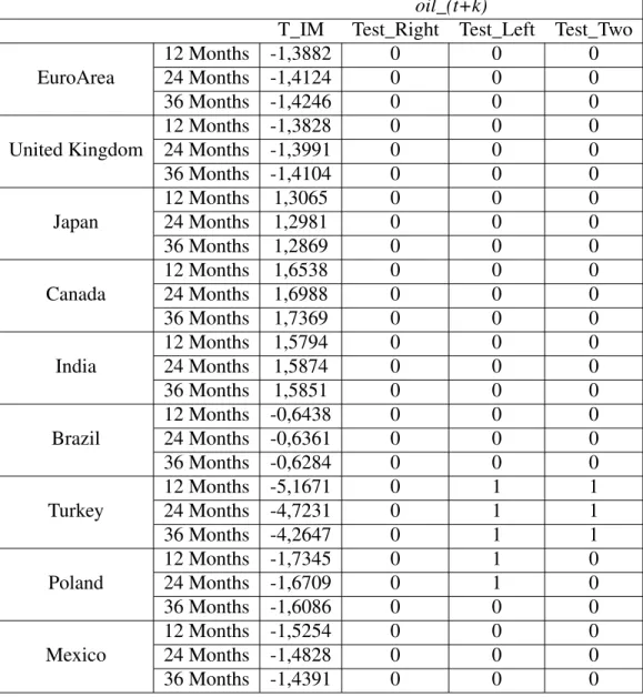
oil_(t+k)
T_IM Test_Right Test_Left Test_Two
EuroArea 12 Months -1,3882 0 0 0 24 Months -1,4124 0 0 0 36 Months -1,4246 0 0 0 United Kingdom 12 Months -1,3828 0 0 0 24 Months -1,3991 0 0 0 36 Months -1,4104 0 0 0 Japan 12 Months 1,3065 0 0 0 24 Months 1,2981 0 0 0 36 Months 1,2869 0 0 0 Canada 12 Months 1,6538 0 0 0 24 Months 1,6988 0 0 0 36 Months 1,7369 0 0 0 India 12 Months 1,5794 0 0 0 24 Months 1,5874 0 0 0 36 Months 1,5851 0 0 0 Brazil 12 Months -0,6438 0 0 0 24 Months -0,6361 0 0 0 36 Months -0,6284 0 0 0 Turkey 12 Months -5,1671 0 1 1 24 Months -4,7231 0 1 1 36 Months -4,2647 0 1 1 Poland 12 Months -1,7345 0 1 0 24 Months -1,6709 0 1 0 36 Months -1,6086 0 0 0 Mexico 12 Months -1,5254 0 0 0 24 Months -1,4828 0 0 0 36 Months -1,4391 0 0 0
10% 20% 30% 40% t-stat beta t-stat beta t-stat beta t-stat beta Eur oAr ea IP 12 1.6565** 0.1828 1.4929 0.1396 1.8148** 0.1648 1.2959 0.1355 24 -0.9974 -0.152 1.3724 0.17 1.0023 0.1213 2.1193** 0.249 36 -1.9739** -0.4047 -1.0597 -0.1561 -1.4694 -0.1981 -0.9728 -0.1285 M1 12 1.0453 0.4178 0.8765 0.2957 1.4322 0.4672 0.2479 0.0754 24 0 0 0.4974 0.17 -0.0005 -0.0002 0 0 36 -0.1348 -0.0791 0.0001 0.0001 -0.5242 -0.204 -0.4781 -0.1728 WTI 12 -0.5972 -0.013 0.2673 0.0051 0.2844 0.0053 0.2067 0.0043 24 -1.7097** -0.04 -0.352 -0.0074 -0.4841 -0.0094 -0.1778 -0.0035 36 -1.2674 -0.0326 -0.5368 -0.0112 -0.5276 -0.0107 -0.2944 -0.0056 United Kingdom IP 12 0.8671 0.6496 1.1086 0.6562 0.0002 0.0001 -0.3269 -0.1637 24 0.7881 0.7371 1.2763 0.8361 0.0303 0.1789 -0.3624 -0.2167 36 0.0697 0.0675 -0.9391 -0.655 0.0008 0.0048 -0.1557 -0.959 M1 12 -0.2549 -0.043 -0.4522 -0.0577 0.2163 0.0247 0.3701 0.0402 24 -0.0869 -0.0143 -0.2776 -0.0358 0.2125 0.2458 0.1855 0.0204 36 -0.6984 -0.1179 -1.3515 -0.1855 0.066 0.0811 0.057 0.0664 WTI 12 -0.2104 -0.0564 -0.1523 -0.03 0.6526 0.106 0.7256 0.1126 24 -1.8404** -0.3915 -1.4615 -0.257 0.1029 0.165 0.2029 0.0307 36 -1.7738** -0.4026 -2.3158** -0.4286 0.0707 0.1199 0.1494 0.24 J apan IP 12 -0.1994 -0.011 -0.9195 -0.0426 0.048 0.0195 0.3118 0.1171 24 -1.1094 -0.0676 -1.1346 -0.0548 -0.3414 -0.1446 -1.3002 -0.5095 36 -1.3501 -0.0935 -1.4013 -0.085 -1.0181 -0.5028 -1.648** -0.0746 M1 12 0.6397 0.2306 0.5554 0.1775 0.3322 0.9014 0.0998 0.2269 24 0.5508 0.1964 0.5568 0.1603 0.2448 0.625 -0.0801 -0.1893 36 0.4834 0.1741 0.5796 0.1773 0.2402 0.6519 -0.577 -0.1457 WTI 12 1.1454 0.0282 1.0574 0.0213 0.4144 0.0743 0.3718 0.063 24 0.1172 0.0029 0.3367 0.0072 -0.1003 -0.019 -0.9731 -0.1654 36 0.3441 0.0086 0.3683 0.0077 -0.0462 -0.0087 -0.8234 -0.0142 Canada IP 12 -2.5008** -0.4151 -1.2417 -0.1723 -1.1414 -0.1503 -0.1512 -0.2024 24 -2.7521** -0.5026 -1.4272 -0.2091 -1.3036 -0.1815 -0.9073 -0.129 36 -3.7315** -0.6219 -1.9054** -0.2946 -2.2601** -0.3362 -1.2755 -0.1918 M1 12 -2.0453** -0.3483 -0.7763 -0.1099 0.0201 0.0026 -0.11 -0.1466 24 -2.1176** -0.3884 -0.63 -0.0945 -0.0224 -0.0031 -0.2008 -0.0283 36 -2.2085** -0.4066 -0.8204 -0.1359 -0.53 -0.0801 -0.2707 -0.0414 WTI 12 -1.4713 -0.2188 -1.3114 -0.1616 -0.5615 -0.0642 0.0098 0.0114 24 -2.9408** -0.4179 -0.7637 -0.0957 0.0113 0.0013 0.158 0.0186 36 -2.6614** -0.379 -1.4282 -0.1782 -0.0361 -0.0041 -0.6148 -0.0705 T able 9: Single V ariable IVX-Q R: De v eloped Econom ies (10% to 40% quantile ). Since the numerical dimens ion of M1 produced v ery lo w v alues for the coef ficients, its dimension w as adjusted so that beta could achie v e suitable v alues.
50% 60% 70% 80% 90% t-stat beta t-stat beta t-stat beta t-stat beta t-stat beta Eur oAr ea IP 12 0.534 0.5666 1.1526 0.1225 0.2236 0.0241 -0.0661 -0.0075 -0.9281 -0.1198 24 1.1073 0.1334 1.1825 0.1428 0.7023 0.0863 0.0001 0 -0.0926 -0.0158 36 -0.3601 -0.0469 -0.0671 -0.0087 0.0874 0.0116 0.2531 0.0382 0.0998 0.0189 M1 12 -0.2935 -0.8705 -0.6158 -0.1799 -0.4677 -0.1396 -1.7464** -0.6282 -2.1423** -0.738 24 -0.4879 -0.1537 -0.7851 -0.2428 -0.5931 -0.1877 -1.7476** -0.6267 -0.7829 -0.2934 36 -0.6102 -0.2149 -1.2649 -0.441 -1.1921 -0.4198 -2.3787** -0.9324 -2.5511** -0.9973 WTI 12 -0.1951 -0.0394 0.3766 0.0076 0.1757 0.0036 -0.074 -0.0017 -0.6189 -0.0166 24 -0.3824 -0.0075 -0.2774 -0.0055 -0.0018 0 -0.9504 -0.0199 -1.7006** -0.0373 36 -0.1344 -0.0025 -0.5244 -0.0098 -0.2739 -0.0052 -1.34 -0.0271 -0.8873 -0.0219 United Kingdom IP 12 -0.5071 -0.2532 -0.7732 -0.3927 -0.6519 -0.341 -1.1915 -0.7308 -0.9121 -0.6959 24 -0.0471 -0.2785 0.0967 0.0578 0.2233 0.1353 0.5003 0.3191 -0.092 -0.0735 36 -0.0001 -0.0007 0.0006 0.0004 0.2385 0.1519 0.4817 0.3196 -0.3531 -0.2844 M1 12 -0.0543 -0.006 -0.906 -0.1014 -1.4849 -0.1644 -1.9211** -0.2227 -1.7366** -0.2301 24 -0.053 -0.0588 -0.9312 -0.1024 -1.455 -0.1592 -1.3348 -0.1497 -1.1402 -0.1689 36 -0.232 -0.2703 -0.7851 -0.0909 -1.456 -0.1681 -1.2128 -0.142 -1.2346 -0.1738 WTI 12 0.0955 0.0152 -0.6194 -0.1004 -0.568 -0.094 -1.4063 -0.2365 -0.9644 -0.2251 24 -0.0288 -0.044 -0.9771 -0.1488 -1.1944 -0.1823 -1.2499 -0.1951 -1.5042 -0.3153 36 -0.1931 -0.31 -0.6895 -0.1113 -1.3853 -0.2218 -1.0653 -0.1765 -1.4387 -0.2719 J apan IP 12 0.0253 0.0108 0.3803 0.1637 0.1938 0.0876 1.0618 0.5247 0.0124 0.0007 24 -0.3667 -0.143 -0.1924 -0.8408 -0.0402 -0.1743 -0.188 -0.0914 -0.9321 -0.0508 36 -0.337 -0.1525 -0.2045 -0.0997 -0.0569 -0.03 -0.2822 -0.1524 -1.8464** -0.1097 M1 12 -0.1788 -0.3944 0.1205 0.3027 -0.2787 -0.7511 -0.3944 -0.9797 -1.8541** -0.548 24 -0.1923 -0.4418 -0.0296 -0.7269 -0.0272 -0.7176 -0.274 -0.7541 -1.8128** -0.5362 36 -0.0887 -0.2202 0.0002 0.0006 -0.3322 -0.9238 -0.2242 -0.6483 -1.9924** -0.6173 WTI 12 -0.073 -0.012 0.1515 0.0253 0.0255 0.0045 -0.0446 -0.0093 0.1147 0.0028 24 -0.8654 -0.1449 -0.381 -0.648 -0.0193 -0.0356 -0.1646 -0.0331 -0.1492 -0.0037 36 -0.5196 -0.0874 -0.8703 -0.1499 -0.4845 -0.0896 -0.1918 -0.0378 -1.0996 -0.0266 Canada IP 12 0.7596 0.1055 0.7298 0.118 0.8814 0.1353 0.9706 0.1482 0.18 0.0289 24 -0.0808 -0.012 0.1029 0.0155 0.7404 0.106 0.8009 0.1125 0.1183 0.0185 36 -0.3116 -0.0492 0.0252 0.0041 0.6575 0.1003 0.4 0.0595 0.2233 0.036 M1 12 0.6346 0.0804 2.3816** 0.2941 1.3322 0.161 1.3995 0.1727 0.7705 0.1059 24 0.3825 0.0537 2.0361** 0.2771 1.2911 0.1704 1.0078 0.1343 0.7753 0.1137 36 0.3621 0.0577 1.9972** 0.3082 1.1736 0.1713 0.9148 0.1358 1.2658 0.2151 WTI 12 0.5672 0.0686 1.9964** 0.2391 1.3393 0.1558 1.9492** 0.229 1.3876 0.1827 24 1.2617 0.1531 2.086** 0.2485 1.2556 0.1456 1.3625 0.1628 2.0815** 0.2742 36 1.1756 0.1398 2.1583** 0.2512 1.2308 0.1403 1.3304 0.1581 1.7112** 0.2169 T able 10: Single IVXQR -de v eloped economies (50% to the 90% quantile). Since the numerical dimension of M1 produced v ery lo w v alues for the coef ficients, its dimension w as adjusted so that beta could achie v e suitable v alues -all v alues of M1 were di vided by 10 12 .