An improved genetic heuristic to support the design of flexible manufacturing systems

(1)

An improved genetic heuristic to support the design of flexible

manufacturing systems

L´ıdia Lampreia Louren¸co

Department of Mathematics, Faculty of Sciences and Technology, New University of Lisbon

Operations Research Centre, Faculty of Sciences, University of Lisbon email:lll@fct.unl.pt

fax: 351 212 948 391

address: Faculdade de Ciˆencias e Tecnologia - Quinta da Torre 2829-516 Monte de Caparica, Portugal

Margarida Vaz Pato

Department of Mathematics, Faculty of Economics and Business Administration, Technical University of Lisbon

Operations Research Centre, Faculty of Sciences, University of Lisbon email:mpato@iseg.utl.pt

address: Instituto Superior de Economia e Gest˜ao - Universidade T´ecnica de Lisboa Rua do Quelhas, 6

(2)

An improved genetic heuristic to support the design of flexible

manufacturing systems

Abstract

In industry, when flexible manufacturing systems are designed within a group technology ap-proach, numerous decision-taking processes appear requiring control of the multiple characteris-tics of the system. In this context, several grouping problems are identified within the scope of combinatorial optimization as is the case of the part families with precedence constraints problem, defined in order to set up families where the total dissimilarity among the parts placed in the same family is minimal and there are precedence constraints when grouping parts as well as capacity constraints. The present paper describes the use of an improved genetic heuris-tic to tackle this problem comprising a standard geneheuris-tic heurisheuris-tic with appropriated operators improved through specific local search. In order to study the performance of the improved ge-netic heuristic, the software CPLEX was used over a binary linear formulation for this problem. Computational results relative to the experiment carried out with test instances partly taken from the literature and others semi-randomly generated, are given. The basic genetic heuristic produced optimal solutions for most of the shortest dimension test instances and the improved version acted positively over more than half of the other instances. Consequently, it seems to be a good tool to tackle high dimensioned test instances where an exact method is not expected to found optimal solution in reasonable computing time.

Keywords: Flexible manufacturing systems; Part families problem; Genetic heuristics.

1. Introduction

In large organisations, the grouping of different elements on the basis of global objectives may be a way whereby specific goals can be more easily attained, by acting on the elements of each group alone. In industry this happens within flexible manufacturing systems, which are designed on the basis of group technology. This may therefore be regarded as an alternative to the technology inherent in conventional production.

These flexible manufacturing systems have the particular feature of sharing a production philoso-phy founded only on orders made. Each order consists of a small batch of products, while a high number of different orders are made at the same period in time. This calls for the introduction of different products, the incorporation of new materials and the adopting of different technological processes, all of which occur at the same time. So as to achieve enhanced competitiveness, the

(3)

need arises for a group-technology based flexible manufacturing system. This should be designed for the efficient processing of small or medium-sized groups of different products, thus assuring a simplification of the productive process, through a reduction in the flow of tools, materials and products handled, besides a resulting saving in production costs.

Two cases follow where such particularities may be seen: one in the micro-electrical industry and another in the metal-cutting industry. For instance, in the Hewlett-Pacard micro-electrical company circuit boards are produced, requiring different components which are inserted in the actual boards using automatic machines whose storage capacity is limited to no more than a given number of components (Hillier and Brandeau [9], Ng [11]). Another case concerns the industrial metal cutting plants. Here a set of computer-controlled tooling machines are required to perform specific operations for the manufacturing of metal parts, using auxiliary components: tools, tool magazine, pallets, fixtures, grippers and equipment to handle parts (Stecke [18]). Here each tool magazine has a limited storage capacity. However, provided the tools are loaded in the magazine, the machine automatically changes one tool for another to perform a different operation.

If we analyse these examples, we find that in both customised productions there is a great variety of types of printed circuit boards or metal parts, in which the number of each type to be produced is small. Another important similarity peculiar to both industries is the fact that there are common components to be inserted in different printed circuit boards, as well as, identical tools to be employed in the manufacturing of different types of parts. Although the number of common components/tools is not that high, it is sufficiently significant to cause this feature to be borne in mind when planning the productive process. Careful structuring of these production systems, by firstly contemplating family grouping of circuit boards that incorporate identical components, and later the production of each family by a same type of machine or cell of machines, helps one to secure considerable gains, in terms of time and energy. This leads to significant final manufacturing profits.

In this context there arises the problem of part families with precedence constraints (PFP) described in the next section. Section 3 is devoted to the improved genetic heuristic that offers good solutions to most instances of the problem, besides taking up little computing time. The encoding of each solution through a chromosome is given, as is the characterization of the genetic operators that modify the chromosome population, besides the improvement local search procedure to be applied to the most fitted chromosomes of the population. Section 4 refers to two mathematical programming models, one of which is quadratic and the other linear, for the PFP. Section 5 concerns the computing experiment undertaken to compare the results of the

(4)

generic heuristics, basic and improved versions, with those obtained by CPLEX in resolving the linear model, and lastly, section 6 presents the conclusions and considerations for future research.

2. The part families with precedence constraints problem

In presenting the problem of part families with precedence constraints, let us consider an indus-trial plant based on a flexible manufacturing system of parts that can either be components or other products for production. We must know the N parts (or batches of parts) ordered and, for each of them, let us call it part i, what tools are used to produce it, its processing time pi,

regarded as independent of the machine, and which parts take precedence over it in terms of production. In this organisation of the productive process, it is agreed to form K (K ≤ N ) part families at the most, and the aim is to ensure that each part family shares similar manufacturing features.

Note that once the families are set up on the strength of the PFP they will be assigned to machines that could well be organised into cells, which gives rise to another problem that is not addressed in this work. As for the problem of machine cell formation see the papers by Ganesh and Srinivasan [5], Chen and Srivastava [2] and Cheng, Goh and Lee [3], and concerning the joint problem of grouping parts into families and the formation of machine cells, considerably neglected in the literature, refer to the paper by Viswanathan [20].

Before beginning the processing of the family-grouped parts, should the machine cells be single, each machine should have previously loaded in its magazine those tools required to perform the various production operations of the parts allotted to it. One should remember that the pro-cessing of a family should be undertaken with no interruptions in swapping tools in the machine magazine. Therefore, there is a limitation to the dimension of the families. The production time of each family also introduces a constraint arising from the machines’ technological requirements. As a result, two types of capacity constraints emerge. One refers to the maximum number of parts Mk allowed in each family k while the other requires that the total production time of the

parts of family k does not exceed the limit parameter Tk. Viswanathan [20] deals precisely with

constraints of this nature, imposed by the number of parts to be assigned to a machine or cell of machines. He points out that this parameter is indicated by the production design analyst. As for the precedence relations between parts, these are caused by the fact that many flexible systems are intended for products requiring activities that occur at different levels of its pro-duction structure. One such example appears in the case of a manufacturing system possessing

(5)

partial assembly and final assembly sections. In such circumstances the parts produced in the manufacturing section are later used to build part assemblies and are applied to the final pro-duct. In this way, some parts may only be incorporated in these unfinished products, if they, besides others, have already been manufactured. A matrix N xN is therefore assumed to be known, its element of line i and of column j, gij, defines the precedence between parts i and j,

in other words, gij =

(

1 if part i directly precedes part j

0 otherwise

So that organisation of the productive process respects the precedence relations between the parts, a specific ordering among the families is stipulated: the grouping of families should be such that the succeeding parts of another for the precedence relations are either placed in families of a higher index than that of the family of the preceding part, or are placed in the same family. Processing of these families will subsequently be undertaken in a rising index order, that is, the parts of a family will only be produced when all the lower index family parts have been produced. A further additional problem, which we shall not deal with now, is that of determining the sequence of the processing of the parts within each family, so as to avoid violation of precedence relations within the family.

The optimisation criteria that determines the grouping of the parts into families concerns mi-nimisation of the sum of dissimilarities among parts within the same family. As previously mentioned, specific tools for each part are used in the production process and the intention is to change tools as little as possible during the production of parts of a family. It is therefore considered that the dissimilarity between two parts i and j, expressed as dij, is the result of the

ratio between the number of different tools and the total number of tools involved in producing these parts: dij = (1/Aij) F X f =1 δ(uif, ujf) where

F - maximum number of tools

Aij - total number of tools required to produce part i and part j

δ(uif, ujf) = ( 1 if uif 6= ujf 0 otherwise with uif = (

1 if tool f is used in processing part i

0 otherwise

Note that the dissimilarity in this case is explained by the Hamming distance, also used in Finke and Kusiak [4] to obtain the costs involved in changing tools in the magazine, but in the context

(6)

of a different problem to that of the present case.

This PFP characterisation was inspired by a problem due, in fact, to Kusiak [10], for which this author presented a p-median type formulation. In this work Kusiak availed himself of the properties of the design of the parts to define the dissimilarity, but he considered neither capacity nor precedence relations. Precedence relations were mentioned [4] by Finke and Kusiak in the formation of part groups. These authors state that in flexible manufacturing systems precedence constraints are far more important than the due date constraints. As was previously mentioned, capacities appear, for instance, in Viswanathan [20]. The PFP was also motivated by the problem proposed by Gunther, Johnson and Peterson [8], where the objective is to attribute to the same work station operations using common tools. However, the PFP was neither formulated nor handled by these authors as it differs from the assembly-line balance problem, which is their main focus of research.

In short, the problem of part families with precedence constraints, known in brief terms as PFP, requires that the grouping of N parts into at the most K families be determined. This would be liable to capacity constraints concerning the number of parts and processing time, besides precedence constraints in forming families. The criterion for grouping selection is given by minimisation of the total dissimilarity among parts within the same family.

The issue is easily defined, however hard to solve, as are many other combinatorial optimisation problems which, as in this case, belong to the NP-hard class. In fact, in Garey and Johnson [6] the NP-hard classification was attributed to a grouping problem, which is a particular case of PFP, when one assumes that only one part precedes all the others and that the capacities, regarding time and the number of parts of each family, are vast enough to allow inclusion of all parts in each family. The use of heuristics, namely of the genetic type, has enabled to find good-quality solutions for many of these difficult problems, at low computing time expenses, Reeves [15]. Remember that production takes place once a set of orders is received and little time is available to plan the new manufacturing system design, which is why the answer must always be promptly found.

In the next section the authors describe the improved genetic algorithm developed for the PFP, by genetically encoding the solutions and respective fitness, so as to create the initial population and also define the selection, crossover and mutation operators. In addition, the local search procedure to improve solutions is also briefly explained.

(7)

3. The improved genetic heuristic

A genetic heuristic may be defined as a random research, applicable to a vast set of optimisation problems of a difficult nature, as is the case of most combinatorial optimisation problems. Un-derlying its origin one finds concepts based on biology and on the theory of evolution (Goldberg [7]).

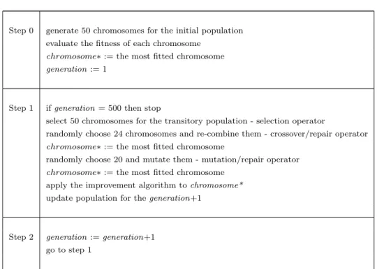
For the problem addressed, the authors propose a genetic algorithm with local search that draws on its specific characteristics. This algorithm, to be seen in summarised form in figure 1, is the product of an improvement to a previous version developed by Louren¸co and Pato [13]. This version differs in terms of the crossover and mutation operators and the attempt to make the solutions feasible after the operators are applied, rather than immediate elimination in the event of non feasibility. It also differs in view of the application of local search from the best solution in all generations, as opposed to the previous version, where local search only acted on the entire population of the last generation of the genetic.

INSERT HERE: ”Figure 1. Improved genetic algorithm”

This genetic algorithm operates with a fixed population of 50 chromosomes, which point to 50 admissible PFP solutions. The initial population is obtained with constructive, improvement algorithms and with randomly conducted processes. From this population the operators act over 500 generations - as explained later. In each generation the crossover operator works on less than half of the population’s chromosomes, and the mutation occurs in 2/5 of the chromosomes at the most.

The chromosomes resulting from crossover and mutation are then analysed as to their feasibility. Should any of the PFP constraints be violated, an attempt is made to repair feasibility. When child-chromosomes are already feasible, following the crossover/repair operation, the parents are replaced by the children only if the offspring are best fitted, whereas, in the mutation/repair situation, the mutants are always inserted in the population. At the end of each generation, the most fitted chromosome, chromosome∗_{, undergoes improvement. In keeping with an elitist}

policy, (Rudolph [16]) besides being preserved as the best chromosome created to date, it is also put back in the population.

After presenting the encoding for the solutions of the PFP and the fitness function, a description of these procedures is given.

(8)

3.1 Encoding

The first step in constructing a genetic algorithm for a given problem is to find a suitable representation scheme for each solution, in other words, to define the respective chromosome. Inclusion or otherwise a part in a family inspires for a possible binary encoding for the solutions, but requires N xK genes. As in the other previous study (Pato and Louren¸co [14]) the authors opted in favour of another encoding, in which each solution is represented through a non-binary vector with only N components - genes - where the position of each gene in the vector represents the index of the part, and the value of the gene represents the index of the family to which the part belongs in the solution in question. By using the appropriate genetic operators, solution feasibility is efficiently maintained, in the majority of cases because the operators do not damage feasibility. Even if they do so, an attempt to built a feasible solution from it is always made through a straightforward procedure.

3.2 Fitness function and selection operator

One must determine the fitness of each chromosome to justify decisions such as keeping it in the population or eliminating it. Fitness of a given chromosome crp is, in this application, given

directly by the following value apt(crp) = N X i=1 N −1_X j=i+1 dij − K X k=1 X i,j∈k i<j

dij, where dij indicates the

dissimilarity between parts i and j, and k is the family index.

Thus the fitness of each chromosome is obtained by subtracting the dissimilarity between the parts placed in the same family from the dissimilarity between all the parts to be grouped together.

The three operators applied in this genetic are that of selection, crossover/repair and muta-tion/repair, so the last two include a feasibility repair procedure. And all are present in each of the generations. Each generation begins with the selection operator acting 50 times to choose the transitory population on which the other two are to act. The purpose behind the existence of selection, in all the generations, is to provide the most fitted chromosomes with a greater possibility of staying in the population and gradually eliminating the less suitable ones. The technique employed to select the transitory population is the roulette.

(9)

3.3 Crossover/repair operator

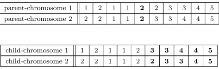
The operator randomly chooses two chromosomes in the transitory population 12 times and, for each pair, determines a crossover point between positions 2 and n − 1. The values of all the genes placed after the crossover point are changed between these two chromosomes, whereas the values of the genes placed before this point remain the same. Consequently, each of the two new chromosomes (child 1 and child 2) stays with the first parts in families of the same index as one of the progenitors and the remaining parts in the families whose index is the same as that of the other progenitor.

Example 1.

Suppose we have 10 parts and 5 families and the precedence relations between the parts are: 1 → 2; 1 → 5; 2 → 7; 3 → 4; 4 → 5; 5 → 6; 6 → 8; 7 → 8; 8 → 9; 9 → 10. Then crossover/repair operator acts for this example as shown in figure 2 below. It is assumed that here both child-chromosomes are already feasible.

INSERT HERE: ”Figure 2. Crossover/repair operator illustration”

This operator proves to be fairly effective in preserving feasibility. However, there can be created violations of precedence constraints or of family capacity, in which case the repair procedure acts in the following way.

One begins by first analysing child-chromosome 1. Should the precedence constraints not be ful-filled, one compares the index of the family of each part that violates the precedence constraints with the indexes of the families of their successors and the violating part is transferred to the family with the lower index of its successors. In this way this violation ceases to exist. The precedence constraints following this correction are verified, although there may occur violation in the families’ capacity. Then, for each of the families in which there is capacity violation, fol-lowing a decreasing index order the parts contained in this family will move to the family whose index immediately follows, until violation ceases to exist. After this repair, child-chromosome 1 is once more analysed as to its feasibility for precedence constraints. If it is already feasible, then its fitness is calculated and it substitutes the less fitted progenitor in the transitory population, if it is better than the latter. Precisely the same procedure acts on child-chromosome 2, in which once its feasibility is recomposed and its fitness calculated, if it is better than that of at least one of the two chromosomes of the current pair, then it substitutes the least suitable.

(10)

progenitors may already have been replaced by child-chromosome 1. This procedure eliminates the descendants, should they fail to meet the readmission requirements or fail to be better than at least one of the progenitors.

One should also add that crossover/repair is applied to the transitory population’s chromo-somes twelve times. In other words, up to twenty-four modifications may be carried out on the chromosomes of a given generation through this operator.

3.4 Mutation/repair operator

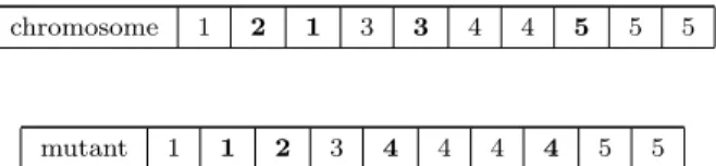
As for the chromosomes that will undergo mutation, these will be randomly selected. In each one four genes are chosen randomly. For each of the first two genes, that is, for the respective parts, one checks for all their successors which is the family with the lowest index in which one of the successors is placed. If the part chosen is in a family which is two or more indexes lower in relation to the index found, then this part reverts to the family whose index is immediately below the one found. Otherwise, the part chosen moves to the family of the index found. As for the two other genes (parts) a similar reasoning is employed, but for the predecessor parts of those chosen. Thus, for each of the parts chosen one determines the highest index from among those of the families to which their predecessors belong. If the part we are addressing is in a family whose index is two units higher, or more, in relation to the determined index, then the part chosen is placed in the family whose index immediately follows it, otherwise it is transferred to the family of this index. Should parts be selected with neither successors nor predecessors, the mutation operator is not applied. The maximum number of mutation/repair operator acts on each generation is twenty.

Example 2. Using the same data of the example 1 the mutation/repair operator is clarified here in figure 3. Let the random positions be: 3, 5, 2 and 8.

INSERT HERE: ”Figure 3. Mutation/repair operator”

Note that the mutation operator does not spoil the precedence constraints between the parts, although it does violate the families’ capacities with a certain degree of frequency. As in the crossover, firstly one tries to repair the capacity constraints violation, and when this happens verification of the mutant with regard to the precedence constraints is analysed once more. Should the mutant be feasible it replaces the original one in the transitory population.

(11)

end of the last generation, the rate of feasible mutants is around 75% of the number of muta-tions undertaken throughout all the generamuta-tions, whereas, in the crossover/repair the number of feasible chromosomes more or less coincides with the total number of chromosomes produced by this operator throughout all the generations.

3.5 Elitism and the improvement heuristic

At the end of each generation an improvement heuristic is applied to the most fitted chromosome, chromosome∗_{. This heuristic analyses transfers of parts of families to others without violating}

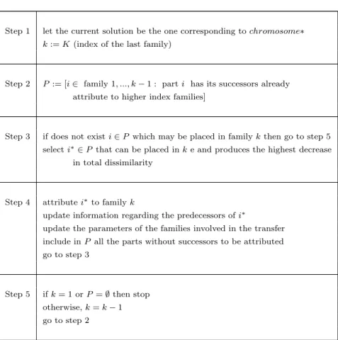
the PFP constraints. By given a specific neighbourhood this may be considered a local search. INSERT HERE: ”Figure 4. Improvement algorithm”

The algorithm briefly described in figure 2 begins by a positioning in the highest index family -current family or family k - while keeping the information of the parts to be found there, besides the respective processing time - Step 1. Once this family is analysed the current one will become the one whose index is immediately below it and successively, in the same way, until family 1. Analysis of the current family - family k - consists in choosing, from among all the parts that are not to be found in this family nor in the higher index families and have no successors to attribute (all successors of i are already assigned to this current family or to the higher index families), for transfer to family k the one that causes the greatest reduction in the total dissimilarity and does not violate the family capacity constraints - Step 3. Let it be part i∗.

Then it updates the information regarding the predecessors of the re-assigned part, the capacities of family k and of the family to whom i∗ _{belonged. Also, for every immediate predecessor of i}∗_,

the number of successors to be attributed falls by one unit, the number of parts of family k is increased by one unit and its processing time is added to the time regarding part i. Lastly, for the family to which the transferred part belonged, the following up-datings are performed: the number of parts is reduced by one unit and total time is reduced by the processing time of i∗. This completes Step 4.

The value of the dissimilarity corresponding to the current solution is also updated.

One now proceeds to the new selection of a part that does not belong to the current family and the process is repeated - Steps 3 and 4 - until all parts of P violate the current family’s capacities or there are no parts with no successors to be attributed in families with an index below k. On

(12)

encountering this situation the current family becomes the family whose index is immediately below, that is, k − 1. When k = 1 or set P becomes empty, then the algorithm ends.

After applying this improvement method to the most fitted chromosome (chromosome∗), the latter is updated, and it is inserted in the transitory population (the next generation population), thus substituting the less fitted one.

One of the products of the improved genetic heuristic is precisely the feasible solution for PFP corresponding to the last updated chromosome∗ _{which, through its total dissimilarity provides}

an upper bound on the optimal value of the PFP. In the following section the authors present mathematical formulations developed so as to test, through the linear relaxation lower bounds, the quality of the heuristic solutions, or even, at least in the case of small instances, solve the PFP itself.

4. Binary formulations

In measuring the total dissimilarity of a solution for PFP one may use a quadratic function of binary variables pointing to the placing of parts in certain families. Should this function be taken as an objective to minimise and the constraints in the building of families be formalised on the basis of the above-mentioned binary variables, the following quadratic formulation is obtained for the part families with precedence constraint problem:

Min K X k=1 N −1_X i=1 N X j=i+1 d_ijx_ikx_jk (4.1) s. to K X k=1 x_ik= 1 i = 1, . . . , N (4.2) K X k=1 kx_ik≤ K X k=1

kx_jk for each pair of parts (i, j) : gij = 1 (4.3) N X i=1 x_ik≤ M_k k = 1, . . . , K (4.4) N X i=1 pixik ≤ Tk k = 1, . . . , K (4.5) x_ik = 0, 1 i = 1, . . . , N ; k = 1, . . . , K (4.6)

The objective function (4.1) represents total dissimilarity, in other words, the sum of the dis-similarity between all the pairs of parts placed in the same family. The set of constraints (4.2)

(13)

requires that each part belong to one family and one family alone. The precedence constraints (4.3) defined for the whole pair of parts (i, j) such that i is an immediate predecessor of j, ensure that if i precedes j then j cannot be placed in a family with an index lower than that of the family in which part i is placed. The cardinality capacity constraints (4.4) do not allow families to be set up with a number of parts above the given limit. Time capacity constraints (4.5) prevent the setting-up of families whose total part processing time exceeds the given time limit. Lastly, the constraints (4.6) associate a given part i to a family k (xik = 1) or otherwise

(x_ik = 0).

The PFP approach through this formulation becomes unviable as a mean of determining the optimal solution as its objective function is quadratic and possesses binary variables. Below it is shown linearisation form of this quadratic formulation.

The introduction of natural variables in the above mentioned binary quadratic formulation enables one to linearise the objective function. Thus, a linear reformulation for the model (4.1)-(4.6) is obtained by substituting the product of variables xikxjk by the natural variable yij and

by a linking in equation, which relates the primitive variables x_ik e x_jk, with the new yij, ∀i < j.

The binary variable yij indicates whether parts i and j are in the same family (yij = 1) or if

they are in different ones (yij = 0), for all i, j = 1, . . . , N, i < j which results in the following

reformulation in mixed linear programming:

Min PN −1_i=1 PN_j=i+1dijyij (4.7)

s. to yij ≥ xik+ xjk− 1 i = 1, . . . , N − 1; j = i + 1, . . . , N ; k = 1, . . . , K (4.8)

constraints (4.2) to (4.6)

yij ≥ 0 i = 1, . . . , N − 1; j = i + 1, . . . , N (4.9)

Constraints (4.8) force each variable yij in the optimal solution to take the value of 1 if i and j

are in the same family. Should these parts be in different families in the optimal solution, the variable yij contributes with the value 0 to the objective function.

This formulation may now be used to solve the PFP by means of standard software, at least for the instances whose dimension is not very high.

(14)

poor, in most instances they are nil. This has to do with the fact that linear relaxation enables each part to remain divided into various fractions of the unit, and these could be attributed to different families. In this way the second member of the constraint (4.8) is negative, which, together with the objective function of the problem, gives rise to the value of the variable yij

in the optimum solution of the linear relaxation be equal to 0. The rare exception to this nil bound result arises when for two parts i and j, the value of yij instead of being 0 is greater

than 0, then there are at least two parts that remain divided, being at least one above 0.5. This case, forces constraint (4.8) to the return a positive value to the variable y_ij and hence the total dissimilarity is not equal to 0.

It should be mentioned that this formulation in binary linear programming was used by Aronson and Klein [1] for a clustering problem applied to software design.

The following section reports on a computational experiment performed with the improved genetic heuristic algorithm and a standard algorithm applied to the formulation (4.2)-(4.9).

5. Computational Experiment

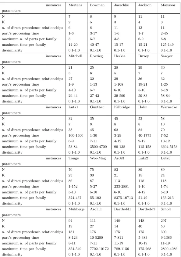
The computacional experiment was carried out with instances partly taken from the literature (Scholl [17]) and from the OR-library [12]. Below, in table 1, the data for these test instances is displayed. Most of the parameters were obtained from the OR-library [12]. As for the other parameters, maximum number of parts per family and dissimilarity, they were (pseudo)randomly generated. Use was made of CPLEX [21] version 6.5 software and the heuristic algorithms were programmed in Pascal. All the algorithms were executed in a 1500 MHz Pentium IV PC with 256 RAM.

INSERT HERE: ”Table 1: Data regarding the test instances”

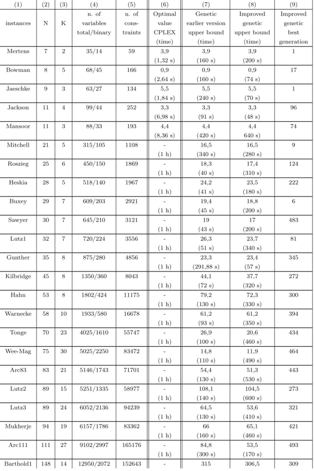
In table 2 information is given on parameters N and K in columns (2) and (3), on the number of variables and constraints (4.2)-(4.6), respectively, in columns (4) and (5), for each instance of the PPF, and some computational results including the execution times, in the others columns. The upper bounds found represent the total dissimilarity corresponding to a genetic earlier version solution and to the improved genetic heuristic solution, columns (7) and (8) respectively. Column (9) indicates the generation where the best solution was find within the improved genetic heuristic. Remember that the number of generations is 500.

(15)

Note that, for the last instance, one was only able, through the algorithm that generates the initial population, to find 10 different chromosomes to form the population. For this reason, it was decided to reduce, in this case, in the improved genetic algorithm, the number of mutations to 5 and the number of crossovers to 10.

An analysis of this table shows that the improved genetic heuristic (colums (8), (9)) had a better performance than the earlier genetic version (column (7)) for most instances without consuming much more computing time, specially where the CPLEX binary linear code failed to operate after a one hour of running time. As for the first five instances both genetic versions gave the optimal solutions.

Let us observe that the generation number where the best feasible solution was found is very hight indicating that the genetic operators are in fact acting along the generations.

CPLEX applied to formulation (4.2)-(4.9) also managed to solve those small instances. However, for the hight dimensioned cases the optimal value is not yet known, also linear relaxation lower bounds are very poor. In fact, the lower bounds from the linear relaxation are 0 for all instances, with the exception of Mertens instance because it has only 2 families, hence each part is divided into two fractions each of them is equal to 0.5 or one is greater than 0.5. This second situation leads to the fact that in the constraint (4.8) the value of yij, for a pair i and j is greater than

0.5. As referred to in section 4, in the case the value of the objective function of the linear relaxation is greater than 0.

If the improved genetic heuristic keeps similar behaviour for the highest dimensions than it showed for the smallest, it will be a very successful non-exact method to tackle this combinatorial optimisation problem. And even if the corresponding upper bounds are not so good, at least it is an easy tool to generate a population of feasible solutions, without consuming a lot of computing time.

Note that the problem studied in Scholl [17] is different from the PFP because it has another objective function, hence it is not possible to compare this paper’s results with his.

6. Closing Comments

This paper presents the part families with precedence constraints problem, within a flexible manufacturing system, for which an improved genetic heuristic is proposed. This hybrid heuristic

(16)

based on a genetic heuristic and on a simple local search procedure gave very good feasible solutions, at least for the cases where the optimum is known. For the others, generated always feasible solutions at low computing expenses. Note that, even for some of the smaller instances tested, the CPLEX failed to obtain the optimal solution.

The improved genetic heuristic may be useful to support flexible production planning with the characteristics given in section 2. In fact, if one considers practical situations in which the total number of parts may reach 5000 (Suresh and Kay [19]), then the part families with precedence constraints problem cannot at the moment, in real time, be optimally solved. Hence, this heuristic may be used for approximately solve the PFP or to be a starting point to develope other methodologies.

References

[1] Aronson, J. E., & Klein, G. (1989). ”A clustering algorithm for computer assisted process organization”. Decision Sciences, 20, 730-745.

[2] Chen, W.-H., & Srivastava, B. (1994). ”Simulated annealing procedures for forming ma-chine cells in group technology”. European Journal of Operational Research, 75, 100-111. [3] Cheng, C. H., Goh, C.-H., & Lee, A. (1996). ”Solving the generalized machine assignment problem in group technology”. Journal of the Operational Research Society, 47, 794-802. [4] Finke, G., & Kusiak, A. (1985). ”Network approach to modelling of flexible manufacturing

modules and cells”. R.A.I.R.O. APII, 19(4), 359-370.

[5] Ganesh, M. V., & Srinivasan, G. (1994). ”A heuristic algorithm for the cell formation problem”. Computers and Industrial Engineering, 26(1), 93-201.

[6] Garey, M. R., & Johnson, D. S. (1979). Computers and intractability: a guide to the teory of NP-completeness. San Francisco: W. H. Freeman and Company, .

[7] Golgberg, D. E. (1989). Genetic algorithms in search, optimization, and machine learning. Massachusetts: Addison-Wesley Publishing Company.

[8] Gunther, R. E., Johnson, G. D. & Peterson, R. S. (1983). ”Currently practiced formula-tions for the assembly line balance problem”. Journal of Operaformula-tions Management, 3(4), 209-221.

[9] Hilllier, M. S. & Brandeau, M. L. (1998). ”Optimal component assignment and board grouping in printed circuit board manufacturing”, Operations Research, 46(5), 675-689.

(17)

[10] Kusiak, A. (1985). ”The part families problem in flexible manufacturing systems”, Annals of Operations Research, 3, 279-300.

[11] Ng, M. (2000). ”Clustering methods for printed circuit board insertion problems”, Journal of the Operational Research Society, 51(10), 1205-1211.

[12] OR-Library, http://www.ms.ic.ac.uk//info.html.

[13] Louren¸co, L. L. & Pato, M. V. (2001). ”A binary linear programming formulation for the part families with precedence constraints problem”. In: Proceedings of the IIE conference. Atlanta: publication of the Institute of Industrial Engineering, production CD-ROM EP Innovations.

[14] Pato, M. V. & Louren¸co, L. L. (1997). ”A standard genetic algorithm for clustering with precedence constraints”. Investiga¸c˜ao Operacional, 17, 71-86.

[15] Reeves, C. R. (1993). Modern heuristic techniques for combinatorial problems. Oxford: Blackwell Scientific Publications.

[16] Rudolph, G. (1996). ”Convergence of Evolutionary Algorithms in General Search Spaces”. In: Proceedings of the 3t_{h IEEE Conference on Evolutionary Computing (pp. 50-54).}

Piscataway (NJ): IEEE Press.

[17] Scholl, A. (1995). Balancing and sequencing of assembly lines. Heidelberg: Physica-Verlag. [18] Stecke, K. E. (1986). ”A hierarchical approach to solving machine grouping and loading problem of flexible manufacturing systems”. European Journal of Operational Research, 24, 369-378.

[19] Suresh, N. C. & Kay, J. M. (1998). Group technology and cellular manufacturing. Boston: Kluwer Academic Publishers.

[20] Viswanathan, S. (1995). ”Configuring cellular manufacturing systems: a quadratic integer programming formulation and a simple interchange heuristic”. International Journal of Production Research, 33(2), 361-376.

(18)

Figure 1. Improved genetic algorithm

Step 0 generate 50 chromosomes for the initial population evaluate the fitness of each chromosome

chromosome∗ := the most fitted chromosome generation := 1

Step 1 if generation = 500 then stop

select 50 chromosomes for the transitory population - selection operator

randomly choose 24 chromosomes and re-combine them - crossover/repair operator

chromosome∗ := the most fitted chromosome

randomly choose 20 and mutate them - mutation/repair operator

chromosome∗ := the most fitted chromosome

apply the improvement algorithm to chromosome* update population for the generation+1

Step 2 generation := generation+1

(19)

Figure 2. Crossover/repair operator illustration

parent-chromosome 1 1 2 1 1 2 2 3 3 4 5 parent-chromosome 2 2 2 1 1 2 3 3 4 4 5

child-chromosome 1 1 2 1 1 2 3 3 4 4 5 child-chromosome 2 2 2 1 1 2 2 3 3 4 5

(20)

Figure 3. Mutation/repair operator

chromosome 1 2 1 3 3 4 4 5 5 5

(21)

Figure 4. Improvement algorithm

Step 1 let the current solution be the one corresponding to chromosome∗

k := K (index of the last family)

Step 2 P := [i ∈ family 1, ..., k − 1 : part i has its successors already

attribute to higher index families]

Step 3 if does not exist i ∈ P which may be placed in family k then go to step 5 select i∗_{∈ P that can be placed in k e and produces the highest decrease}

in total dissimilarity

Step 4 attribute i∗_{to family k}

update information regarding the predecessors of i∗

update the parameters of the families involved in the transfer include in P all the parts without successors to be attributed go to step 3

Step 5 if k = 1 or P = ∅ then stop otherwise, k = k − 1 go to step 2

(22)

Table 1: Data regarding the test instances

instances Mertens Bowman Jaeschke Jackson Mansoor parameters

N 7 8 9 11 11

K 2 5 3 4 3

n. of direct precedence relationships 6 8 11 13 11 part’s processing time 1-6 3-17 1-6 1-7 2-45 maximum n. of parts per family 5 5-7 3-8 6-9 6-8 maximum time per family 14-20 40-47 15-17 15-21 125-149 dissimilarity 0.1-1.0 0.1-1.0 0.1-1.0 0.1-1.0 0.1-1.0

instances Mitchell Roszieg Heskia Buxey Sawyer parameters

N 21 25 28 29 30

K 5 6 5 7 7

n. of direct precedence relationships 27 32 39 36 32 part’s processing time 1-9 1-13 1-108 19-21 1-25 maximum n. of parts per family 4-10 5-7 6-10 5-10 6-18 maximum time per family 29-44 27-42 39-590 59-83 58-84 dissimilarity 0.1-1.0 0.1-1.0 0.1-1.0 0.1-1.0 0.1-1.0

instances Lutz1 Gunther Kilbridge Hahn Warnecke parameters

N 32 35 45 53 58

K 7 8 8 8 10

instances Tonge Wee-Mag Arc83 Lutz2 Lutz3 parameters

N 70 75 83 89 89

K 23 30 21 15 24

instances Mukherje Arc111 Barthold1 Barthold2 Scholl parameters

N 94 111 148 148 297

K 19 27 14 40 50

(23)

Table 2: Results of the computational experiment

(1) (2) (3) (4) (5) (6) (7) (8) (9) n. of n. of Optimal Genetic Improved Improved instances N K variables cons- value earlier version genetic genetic

total/binary traints CPLEX upper bound upper bound best (time) (time) (time) generation Mertens 7 2 35/14 59 3,9 3,9 3,9 1 (1,32 s) (160 s) (200 s) Bowman 8 5 68/45 166 0,9 0,9 0,9 17 (2,64 s) (160 s) (74 s) Jaeschke 9 3 63/27 134 5,5 5,5 5,5 1 (1,84 s) (240 s) (70 s) Jackson 11 4 99/44 252 3,3 3,3 3,3 96 (6,98 s) (91 s) (48 s) Mansoor 11 3 88/33 193 4,4 4,4 4,4 74 (8,36 s) (420 s) 640 s) Mitchell 21 5 315/105 1108 - 16,5 16,5 9 (1 h) (340 s) (280 s) Roszieg 25 6 450/150 1869 - 18,3 17,4 124 (1 h) (40 s) (310 s) Heskia 28 5 518/140 1967 - 24,2 23,5 222 (1 h) (41 s) (180 s) Buxey 29 7 609/203 2921 - 19,4 18,8 6 (1 h) (45 s) (200 s) Sawyer 30 7 645/210 3121 - 19 17 483 (1 h) (43 s) (200 s) Lutz1 32 7 720/224 3556 - 26,3 23,7 81 (1 h) (51 s) (340 s) Gunther 35 8 875/280 4856 - 23,3 23,4 345 (1 h) (291,88 s) (57 s) Kilbridge 45 8 1350/360 8043 - 44,1 37,7 272 (1 h) (72 s) (320 s) Hahn 53 8 1802/424 11175 - 79,2 72,3 300 (1 h) (130 s) (330 s) Warnecke 58 10 1933/580 16678 - 61,2 61,2 394 (1 h) (93 s) (350 s) Tonge 70 23 4025/1610 55747 - 26,9 20,6 434 (1 h) (100 s) (460 s) Wee-Mag 75 30 5025/2250 83472 - 14,8 11,9 464 (1 h) (110 s) (490 s) Arc83 83 21 5146/1743 71701 - 54,4 51,3 443 (1 h) (130 s) (530 s) Lutz2 89 15 5251/1335 58977 - 108,1 104,5 273 (1 h) (140 s) (600 s) Lutz3 89 24 6052/2136 94239 - 64,5 53,6 321 (1 h) (130 s) (410 s) Mukherje 94 19 6157/1786 83362 - 66 65,1 421 (1 h) (160 s) (460 s) Arc111 111 27 9102/2997 165176 - 84,8 53,5 493 (1 h) (300 s) (170 s) Barthold1 148 14 12950/2072 152643 - 315 306,5 309

(24)

(1 h) (220 s) (400 s)

Barthold2 148 40 16798/5920 435523 - 84,9 78,5 493 (1 h) (230 s) (340 s)

Scholl 297 50 58806/14850 2198497 - 319,5 304,7 467 (1 h) (320 s) (240 s)