Dry Markets and Superreplication Bounds of
American Derivatives
João Amaro de Matos
1and Ana Lacerda
2Faculdade de Economia
Universidade Nova de Lisboa
Campus de Campolide
1099-032 Lisbon, Portugal
October 13, 2004
1Corresponding author. Email: amatos@fe.unl.pt. Phone:+351962406397. 2Financial support from Fundação Amélia de Mello, INOVA and CMA-FCT is
Abstract
This paper studies the impact of dry markets for underlying assets on the pricing of American derivatives, using a disrete time framework. Dry mar-kets are characterized by the possibility of non-existence of trading at certain dates. Such non-existence may be deterministic or probabilistic. Using su-perreplicating strategies, we derive expectation representations for the range of arbitrage-free values of the dervatives. In the probabilistic case, if we consider an enlarged filtration induced by the price process and the market existence process, ordinary stopping times are required. If not, randomized stopping times are required. Several comparisons of the ranges obtained with the two market restrictions are performed. Finally, we conclude that arbitrage arguments are not enough to define the optimal exercise policy.
Keywords: American derivatives, pricing, incomplete markets, dry mar-kets, superreplication, randomized stopping times, strong duality.
1
Introduction
Among the traditional assumptions on which derivatives’ pricing is based, markets are perfect and the underlying asset can be transacted at any point in time. Under the absence of arbitrage opportunities the value of a derivative can be computed as the value of a portfolio on the underlying risky asset and risk-free bonds that exactly replicates its payoff. Such portfolio can be rebalanced in a self-financing way until the maturity of the derivative, by continuously transacting the underlying asset and the bonds. Under these assumptions, the calculated value of the initial portfolio can be shown to be the equilibrium price of the derivative. Considering the case of American derivatives it has been shown by Bensoussan (1984) and Karatzas (1988) that, in this setting, the no-arbitrage value of one such derivative is indeed the supremum of the implied European derivative values over all possible stopping times.
In this paper we assume that an American derivative and its respective underlying asset cannot be transacted at some points in time, and study the impact of this constraint on the pricing of American derivatives. The fact that the assets can be transacted only at some points in time can be described as a lack of liquidity of the market, as in Longstaff (2001). We shall refer to this situation as dry markets. We will consider two different types of dry markets. In the first type, to be called deterministic illiquidity, we know ex-ante exactly at which points in time markets do exist or do not exist. In the second type, to be called probabilistic illiquidity, we assign a probability p to the existence of the market at each point in time.
Markets’ dryness implies that markets may become incomplete in the sense that perfect hedging of the derivative in all states of nature is no longer possible. However, for any given derivative, portfolios can be found that have the same payoff as the derivative in some states of nature and higher payoffs in the other states. Such portfolios are said to be superreplicating (or super-hedging). Holding one such portfolio should be worth more than the deriva-tive itself and therefore, the value of the cheapest of such portfolios should be seen as a bound on the value of the derivative. The nature of the superrepli-cating bounds for European derivatives is well characterized in the context of incomplete markets in the papers by El Karoui and Quenez (1991,1995), Edirisinghe, Naik and Uppal (1993) and Karatzas and Kou (1996). A direct application to the case of European option pricing when the market for the underlying is dry can be found in Amaro de Matos and Antão (2001). As all these results stress, under market incompleteness the hedging position of a market-maker is different depending on whether this intermediary is in a long or in a short position. This fact results in a lower and an upper bound
for the derivatives’ values.
The superreplicating bounds establish the limits of the interval for the prices outside which the market-maker has a positive profit with probability one. In other words, an arbitrage opportunity exists if the market-maker sells options above the upper bound or buys options below the lower bound. There has been a relatively extensive literature in the continuous time setting, analyzing this problem and characterizing in varying degrees of gen-erality the superhedging bounds of American derivatives in incomplete mar-kets. Examples are the papers by Kramkov (1996), Follmer and Kramkov (1997), Follmer and Kabanov (1998) and Karatzas and Kou (1998). More recently, a paper by Jha and Chalasani (2001) discuss the particular case of transaction costs in discrete time and conclude that, in their specific setting, the superreplicating bounds of one such derivative may also be written as the supremum of the implied European derivative value. However, there are two important subtleties in their result: first, the supremum in this case must be taken over randomized stopping times and second, the probability measure defining the European value over which the supremum is taken, may depend itself on the randomized stopping time that solves the problem.
Jha and Chalasani (2001) relate their result to the fact that1, under
in-complete markets, the choice of exercise policy may influence the charac-terization of the marketed subspace, and therefore influence the pricing of securities. A rational exercise policy may even not be well defined if the state-price deflator depends on the exercise policy. This argument would pro-vide solid ground for the optimal randomized stopping times characterizing the superreplication bounds of the American derivatives under proportional transaction costs.
Our results show that, under dry markets, and in the same general dis-crete time setting used by Jha and Chalasani (2001), we can also write the superreplicating bounds of an American derivative as the supremum of the implied European derivative value. However, the supremum in this case may be taken over deterministic stopping times, as opposed to the intuition provided by the above cited authors. Although the result for deterministic illiquidity may be understood in the context of the superreplicating bounds discussed in Harrison and Kreps (1979), the case of probabilistic illiquidity is of a different nature since it crosses an additional source of uncertainty (existence or non existence of the market at a given point in time).
Our work is organized as follows. Section 2 models the case of Determin-istic Illiquidity, introducing the model and relevant probabilDetermin-istic concepts. Section 3 states the corresponding results, presenting the upper and lower
superreplicating bounds of American derivatives. This is followed by Sec-tion 4 that models the case of Probabilistic Illiquidity, after what SecSec-tion 5 presents the corresponding results for the upper and lower superreplicating bounds of American derivatives. In section 6 these different bounds are com-pared. The exercised policy in dry markets is discussed in section 7. Finally, we section 8 we conclude. Our main technical proofs are presented in the Appendix.
2
Deterministic Illiquidity
2.1
The model
Consider an economy where three different assets are transacted. The first asset is a risk free asset with unitary initial value that provides a certain total return of R per period; the second asset to be considered is a risky asset (the stock); finally, the third asset is an American derivative, written on the stock, with expiration date T. We work in discrete time, corresponding to dates 0, 1, ..., T. The set of these dates is denoted by T ≡ {0, 1, . . . , T } . The evolution of the value of the underlying asset is modelled by means of a finite event tree. Each node of such tree is identified by a pair (j, t) , where j denotes the j-th node at time t. There is only one node at time t = 0, denoted by (0, 0) . For any given node (j, t) , the set of successors at time t + k, k > 0, is denoted by jt+(t + k). For simplicity let jt+ denote the set of
immediate successors, i.e., jt+ ≡ j +
t (t + 1). The nodes (j, T ) , at time T, are
called terminal nodes and jT+ is assumed to be the empty set ∅. It is also assumed that, for t < T , each nonterminal node (j, t) has a nonempty set of immediate successors, i.e., jt+6= ∅. In an analogous way, the set of immediate
predecessors of a node (j, t) 6= (0, 0) is denoted by jt−. In what follows we
shall consider the case where such sets jt− have a unique element. Moreover,
we denote by Jt the set of all nodes at any point in time t
Jt=∪j (j, t) .
A path on the event tree is a set of nodes w = ∪t∈{0,1,...,T }(jt, t) such that
each element in the union satisfies (jt+k, t + k)∈ jt+(t + k) , with k > 0 and
t + k ∈ {0, 1, ..., T } . Let Ω denote the set of all paths on the event tree. Each node in the tree represents the set of all tree paths that contain that node. Let S denote the process followed by the stock price. More precisely, let S (j, t) denote the price of the stock at node (j, t) . A natural filtration on the space Ω associated to the price process S is F = F0, F1, . . . , FT,where
random variable will be defined in the measurable space (Ω, F). Similarly, let G denote the process followed by the payoff of American derivative. Hence, G (j, t) denotes the payoff of the American derivative at node (j, t) whenever exercised at that point. Let ¯S (j, t) and ¯G (j, t) stand for the discounted values of the above processes, i.e.,
¯
G (j, t) = G (j, t)
Rt and ¯S (j, t) =
S (j, t) Rt .
Dry markets are characterized by the fact that transactions are possible only at some points in time. We hereby model dry markets allowing trans-actions only at times t in a set Tm ⊆ T . It is also assumed that transactions
are possible at times t = 0 and t = T , i.e., {0, T } ⊆ Tm.
At any node (j, t) consider the portfolio constituted by ∆ (j, t) shares of the underlying asset and an amount B (j, t) invested in the risk free asset. One such portfolio is denoted by [∆ (j, t) , B (j, t)]. Its value process is given by
V (j, t) = ∆ (j, t) S (j, t) + B (j, t) .
Consider a short position on the American derivative. A replicating strat-egy is a sequence of portfolios {[∆ (j, t) , B (j, t)]}t∈Tm such that the value of
each of them is larger than or equal to the payoff of the derivative at any non-terminal node in the next transaction time. Additionally, at any termi-nal node its value is equal to the payoff of the derivative. In other words, for any two consecutive trading dates t1 and t2 > t1, consider an arbitrary
node (j, t1) and the subset of its possible successors jt+1(t2) Then, the
port-folio at t1, [∆ (j, t1) , B (j, t1)] , must be such as to generate in t2 a value
∆ (j, t1) S (i, t2) + B (j, t1) Rt2−t1 such that
∆ (j, t1) S (i, t2) + B (j, t1) Rt2−t1 ≥ G (i, t2)
with (i, t2)∈ jt+1(t2) and if t2 = T then
∆ (j, t1) S (i, T ) + B (j, t1) RT −t1 = G (i, T ) .
A self-financed portfolio is a portfolio that generates enough wealth to rebal-ance the portfolio according to any future state of nature. In other words, for any two consecutive trading dates t1 and t2 > t1, consider an arbitrary
node (j, t1)and the set of its possible successors
©
(i, t2) : i∈ jt+1
ª
.Then, the value of the portfolio at that point in time, ∆ (j, t1) S (j, t1) + B (j, t1)must
be such as to generate
For a long position on the American derivative, analogous definitions are obtained with reverted inequalities, but only for the nodes (i, t) such that the option would be exercised, i.e., such that G (i, t) > V (i, t) .
If a complete market is considered the value of an American derivative is the value of the cheapest self-financing portfolio on the underlying risky asset and risk-free bonds that replicates the payoff of the American derivative. For this portfolio the following condition will hold at any non-terminal node
∆ (j, t1) S (i, t2) + B (j, t1) Rt2−t1 = max [V (i, t2) , G (i, t2)] .
In dry markets, however, the number of transacted securities may be in-sufficient to allow the construction of a self-financing portfolio that replicates the payoff of an American derivative. In other words, markets may become incomplete. In that case, there is not a unique arbitrage free value for the American derivative. However, replacing the notion of replicating strategy by the notion of superreplication strategy it is possible to derive an arbitrage free range of variation for the value of the American derivative. In order to find the upper bound of this range consider a short position in the derivative. The upper bound will be the value of the cheapest portfolio that the buyer of the derivative can buy in order to completely hedge against any possibility of exercise of the American derivative and without need of additional financing at any rebalancing dates. Note that in order to completely hedge against the possibility of exercise the value of the portfolio, at any given node, has to be equal or higher than the payoff of the American derivative. In that case it is said that the portfolio superreplicates the payoff of the American derivative. On the other hand, in order to find the lower bound of the arbitrage-free range of variation consider a long position in the derivative. For a given exercise policy consider the most expensive portfolio that the buyer of the American derivative can buy in order to be fully hedged. The lower bound is the value of the most expensive portfolio chosen among the portfolio just described. Note that in this case the buyer of the American derivative is, for a given exercise policy, completely hedged if in any node where the option may be exercised the payoff of the American derivative is higher than the value of the hedging portfolio. In this case it is said that the portfolio is superreplicated by the American derivative.
Under market completeness, both limiting portfolios coincide with a repli-cating portfolio and the value of the derivative is well characterized [Karatzas (1988)]. Under market incompleteness however, that is no longer true and the arbitrage-free value of the derivative must lie between the values of the two limiting superreplicating portfolios.
In what follows we are going to characterize the upper and lower arbitrage-free bounds for the value of the American derivatives in the framework
de-scribed above. In order to do that, we first define some mathematical objects, such as node probability measure, adjusted probability measure and stopping time.
2.2
Some Probabilistic Definitions
Definition 2.1 A node probability measure is a nonnegative node func-tion q (j, t) such that
X
t∈Tm
X
(j,t)∈Jt
q (j, t) = 1.
The set of all node probability measures is denoted by Q.
Definition 2.2 A node probability measure on the event tree is said to be simple if, for t ∈ Tm and t + k ∈ Tm , there are no two nodes in the
same path, say (i, t) and (j, t + k) ∈ i+t (t + k) , such that q (i, t) > 0 and
q (j, t + k) > 0.
The following theorem is analogous to theorem 6.7 of Jha and Chalasani (2001) but now in the framework of dry markets.
Theorem 2.1 (Jha and Chalasani) The extreme points of the set of nodes Q are simple node probability measures, i.e., on every path on the event tree there is at most one node where q is strictly positive.
The proof of this theorem follows closely the proof of theorem 6.7 in Jha and Chalasani (2001) and is presented in the appendix A.
Definition 2.3 An adjusted probability measure is a nonnegative func-tion P (i, t) such that P (0, 0) = 1 and for all t ∈ Tm
P (i, t) = X
(j,s)∈i+(s)P (j, s)
with s = min {z ∈ Tm : z > t} .
The set of all probability measures is denoted by P.
Definition 2.4 A process Z = {Zt: t∈ Tm} is called adapted to the
Let τ denote an ordinary stopping time that takes values in Tm, i.e., τ
is a map such that τ : Ω → Tm and {w : τ (w) ≤ t} ∈ Ft for all t ∈ Tm. We
define a nonnegative adapted process Xτ associated with τ that is defined
for all t ∈ Tm and has the form Xτ(i, k) = 1 if τ (w) = k and Xτ(i, k) = 0
otherwise, where (i, k) is a node in path w. Let T and XT denote the set of
all τ and associated Xτ, respectively.
Definition 2.5 A simple node probability measure is said to be associated with a given stopping time if at any node such that Xτ(i, k) is equal to zero
then q (i, t) is also equal to zero. Moreover, at any node such that Xτ(i, k) is
strictly positive then q (i, t) is also positive.
The set of all node probability measures with this property is denoted by Qτ.
Definition 2.6 For any adjusted probability measure P ∈ P and stopping time τ ∈ T we say that P is a τ-martingale measure if, P -almost surely, for any (i, t) with t ∈ Tm we have
X m>t,m∈Tm X (j,m)∈i+t(m) p (j, m) Xτ(j, m) £¯ S (i, t)− ¯S (j, m)¤= 0 The set of all P that have this property is denoted by P (τ) .
Definition 2.7 For any adjusted probability measure P ∈ P we say that P is a martingale measure if, P -almost surely, for any (i, t) ∈ Jt with t ∈ Tm
we have X m>t,m∈Tm X (j,m)∈i+t(m) p (j, m)£S (i, t)¯ − ¯S (j, m)¤= 0 The set of all P that have this property is denoted by P.
Let (P, Xτ) denote a measure-strategy pair, i.e., a pair constituted by an
adjusted probability measure and a nonnegative adapted process.
Definition 2.8 A measure-strategy pair (P, Xτ) is said to be equivalent to
a node probability measure if P (i, t) Xτ(i, t) = q (i, t) for any given node (i, t)
Theorem 2.2 (Jha and Chalasani) Let (P, Xτ) be a measure-strategy pair.
The simple node function q defined by q (i, t) = P (i, t) Xτ(i, t) is the unique
equivalent node-measure. Conversely, for a given simple node probability measure, q, there is a measure-strategy pair (P, Xτ) equivalent to q, where P
is uniquely defined at nodes (i, t) where q (i, t) +P(j,τ )∈i+ t(τ )
τ >t, τ ∈Tm
q (j, τ ) > 0, and Xτ is uniquely defined at nodes (i, t) where q (i, t) > 0.
A version of the proof of this result, adjusted to case of dry markets, is provided in Appendix A.
3
Results on Deterministic Illiquidity
3.1
Upper bound for the Value of an American
Deriva-tive
The upper bound for the value of an American derivative is the maximum value for which the derivative would be transacted without allowing for ar-bitrage opportunities. In order to find the upper bound consider a short position in the derivative. The maximum value for which the derivative would be transacted without allowing for arbitrage opportunities would be the value of the cheapest portfolio that the buyer of the derivative can buy in order to completely hedge against any possibility of exercise of the Amer-ican derivative and without need of additional financing at any rebalancing dates. A portfolio is initially built such that, at each transaction date un-til maturity, it generates enough wealth, so as to be rebalanced according to any revealed state of nature. Since by construction there is no need of additional financing, one such strategy is said to be a self-financed strategy. Additionally, it has to be a superreplicating strategy, i.e., a sequence of port-folios {[∆ (j, t) , B (j, t)]}t∈Tm such that their values are greater or equal to
the payoff of the derivative at any node in the next transaction time. In other words, for any two consecutive trading dates t1 and t2 > t1, consider an
arbi-trary node (j, t1) and the subset of its possible successors jt+1(t2) .Then, the
portfolio at t1, [∆ (j, t1) , B (j, t1)] ,must be such as to generate in t2 a value
∆ (j, t1) S (i, t2) + B (j, t1) Rt2−t1 such that
∆ (j, t1) S (i, t2) + B (j, t1) Rt2−t1 ≥ G (i, t2) , (1)
with (i, t2)∈ jt+1(t2) .
More formally, take any t1 ∈ Tm,such that t1 6= T . Define the consecutive
of the American derivative can thus be seen as the solution of the following problem: Vdu = min {∆(j,t),B(j,t)} (j,t)∈Jt t∈Tm\{T } ∆ (0, 0) S (0, 0) + B (0, 0)
subject to the superreplicating restrictions:
∆ (0, 0) S (0, 0) + B (0, 0)≥ G (0, 0) , (2)
∆ (j, t1) S (i, t2) + B (j, t1) Rt2−t1 ≥ G (i, t2) , (3)
for all t1 ∈ Tm\ {T } and (i, t2)∈ j+(t2) with t2 = min (s∈ Tm : s > t1) and
subject to the self-financing restrictions:
∆ (j, t1) S (i, t2) + B (j, t1) Rt2−t1 ≥ V (i, t2) (4)
for all t1 ∈ Tm\ {max {t ∈ Tm : t < T} , T } and (i, t2) ∈ j+(t2) with t2 =
min (s ∈ Tm\ {T } : s > t1) .
Using results from linear programming the upper bound arbitrage free bound of the American derivative can be written as follows.
Theorem 3.1 There exists a node probability measure q ∈ Q such that the upper hedging price of an American derivative in a dry market can be written as Vdu = max q∈Q X t∈Tm X (j,t) q (j, t) ¯G (j, t)
such that for any (i, t) with t ∈ Tm
X
m>t,m∈Tm
X
(j,m)∈i+t(m)
q (j, m)£S (i, t)¯ − ¯S (j, m)¤= 0.
Proof. As the problem that must solved in order to find the upper bound of the American derivative is a linear programming problem it is possible to construct its dual. Let λ (0, 0) , λ (i, t2) and α (i, t2) be the dual variables
associated with restrictions (2), (3) and (4), respectively. Then, the dual problem is
maxX
t∈Tm
subject to
λ (0, 0) S (0, 0) +X
(i,t)∈i+0(t)
[λ (i, t) + α (i, t)] S (i, t) = S (0, 0) (5)
λ (0, 0) +X (i,t)∈i+0(t) [λ (i, t) + α (i, t)] Rt= 1 (6) with t = min (s ∈ Tm : s > 0) , X (j,t2)∈i+t1(t2) S (j, t2) [λ (j, t2) + α (j, t2)]− α (i, t1) S (i, t1) = 0 (7) X (j,t2)∈i+t1(t2) [λ (j, t2) + α (j, t2)] Rt2−t1 − α (i, t1) = 0 (8)
for all t1 ∈ T \ {0, max {s ∈ Tm: s < T} , T } and t2 = min (s∈ Tm : s > t1) ,
and, finally, X (j,T )∈i+t(T ) S (j, T ) λ (j, T )− α (i, t) S (i, t) = 0 (9) X (j,T )∈i+(T )S (j, T ) R T −t− α (i, t) = 0 (10)
for all t = max {s ∈ Tm : s < T} .
Note that the restrictions (5), (7) and (9) of the dual problem are asso-ciated with the variables ∆ (0, 0) , ∆ (i, t1) and ∆ (i, t) , respectively, of the
primal problem. In a similar way, the restrictions (6), (8) and (10) are, re-spectively, associated with the primal variables B (0, 0) , B (i, t1)and B (i, t).
The restrictions presented in equations (7) and (9) can be rewritten such that, for all t ∈ Tm\T, we have
X (j,m)∈i+t(m) m>t,m∈Tm λ (j, m) Rm−tS (i, t) =X(j,m)∈i+(m) m>t,m∈Tm λ (j, m) S (j, m) , (11)
From equations (6), (8) and (10) we obtain X
(i,t) t∈Tm
λ (i, t) Rt= 1 (12)
Considering equations (12), (5) and (12), we have, for all (i, t) , X (j,m)∈i+(m) m>t,m∈Tm λ (j, m) Rm−tS (i, t) =X(j,m)∈i+(m) m>t,m∈Tm λ (j, m) S (j, m) .
Let q (i, t) = λ (i, t) Rt. For any t ∈ Tm\ {T } , X (j,m)∈i+(m) m>t,m∈T q (j, m) ¯S (i, t) =X(j,m)∈i+(m) m>t,m∈T q (j, m) ¯S (j, m) .
Hence, the dual problem can be written as
max q∈Q X (i,t)∈Jt t∈Tm q (i, t) ¯G (i, t)
such that for any (i, t) with t ∈ Tm
X
m>t,m∈Tm
X
(j,m)∈i+t(m)
q (j, m)£S (i, t)¯ − ¯S (j, m)¤= 0.
The upper bound solving the problem above can also be seen as the solution of a more intuitive problem. In fact, it can be shown that this upper bound maximizes over all possible stopping times the expected discounted payoff, when the expectation is optimized among all adjusted probability measures. In other words,
Theorem 3.2 There exists an adjusted probability measure P ∈ P (τ) and an adapted process Xτ ∈ XT such that the upper hedging price of an American
derivative in a dry market can be written as Vdu = max
τ ∈T P ∈P(τ )max E pG
τ
with Gτ(i, t) = Xτ(i, t) G (i, t) . Additionally, if there is a probability measure
with positive probability on every path then the upper hedging price of an American derivative in a dry market can be rewritten as
Vdu = max
τ ∈T maxP ∈P E pG
τ
where Gτ(i, t) = Xτ(i, t) G (i, t) , as before.
Proof. As Q is a convex set, the maximum of the problem max q∈Q X (i,t)∈Jt t∈Tm q (i, t) ¯G (i, t)
such that for any (i, t) with t ∈ Tm
X
m>t,m∈Tm
X
(j,m)∈i+t(m)
is obtained at the extremes points of Q.
By theorem (2.1) we know that the extremes points are simple node measures. Using theorem (2.2) we can rewrite the problem above as
max τ ∈T P ∈P(τ )max E pG¯ τ (13) where ¯
Gτ(i, t) = ¯G (i, t) Xτ(i, t) .
As stressed in Jha and Chalasani (2001), page 64, if there is a martingale measure ˆP ∈ P with positive measure on every path, w, the inner maxi-mization in (13) can be restricted to all P ∈ P without affecting its value. First, any P ∈ P also belongs to P (τ) . Second, any measure P ∈ P can be redefined to be a martingale measure P0 ∈ P (τ) such that EP0G¯τ = EPG¯τ,
as follows
P0(i, t) = (
P (i, t) , t ≤ k : if (i, t) ∈ w and τ (w) = k P0 −(i, t) ˆ P (i,t) ˆ P−(i,t) otherwise where P0
−(i, t) and ˆP−(i, t) are the probabilities in the node that is an
im-mediate predecessor of (i, t) .
3.2
Lower bound for the Value of an American
Deriva-tive
The lower bound for the value of an American derivative is the minimum value for which the derivative would be transacted without allowing for arbi-trage opportunities. In order to find the lower bound consider a long position in the derivative. As stressed in Karatzas and Kou (1998) while the seller of the American derivative has to be hedged against any possible exercise pol-icy, the buyer of the American derivative needs only to hedge against a given exercise policy that is defined by himself. For a given exercise policy consider the most expensive portfolio that the buyer of the American derivative can buy in order to be fully hedged and without need of additional financing at any rebalancing dates. The minimum value for which the derivative would be transacted without allowing for arbitrage opportunities would be the value of most expensive portfolio chosen among all the portfolios just mentioned.
For any given exercise policy τ and any node (j, t), such that (j, t) is before the exercise time, consider the portfolio constituted of ∆τ(j, t)shares
For each exercising policy we are looking for the most expensive portfolio that the buyer of the American derivative can buy that is self-financed and is supperreplicated by the payoffs of the American derivative. A portfolio [∆τ(j, t
1) , Bτ(j, t1)] is said self-financing if, for any two consecutive trading
dates t1 and t2 > t1 and an arbitrary node (j, t1), the portfolio is such as to
generate in t2 a value ∆τ(j, t1) S (i, t2) + Bτ(j, t1) Rt2−t1 such that
∆τ(j, t1) S (i, t2) + Bτ(j, t1) Rt2−t1 ≤ Vτ(i, t2) , (14)
for any node (i, t2) ∈ jt+1(t2) before the exercise of the American derivative.
Additionally, a portfolio [∆τ(j, t1) , Bτ(j, t1)]is said to be superreplicated by
Gτ(i, t2)if, for any two consecutive trading dates t1 and t2 > t1 and an
arbi-trary node (j, t1) ,it generates in t2 a value ∆τ(j, t1) S (i, t2)+Bτ(j, t1) Rt2−t1
such that
∆τ(j, t1) S (i, t2) + Bτ(j, t1) Rt2−t1 ≤ Gτ(i, t2) , (15)
for any (i, t2) ∈ jt+1(t2) when it is optimal to the holder of the American
option to exercise it given τ . The minimum value for which the derivative would be transacted without allowing for arbitrage opportunities would be the value of the most expensive portfolio chosen among all stopping times.
The lower bound for the value of the American derivative can thus be seen as the solution of the following problem:
Vdl = max
τ ∈T {∆τ(j,t),Bmaxτ(j,t)}∆τ(0, 0) S (0, 0) + Bτ(0, 0)
subject to the superreplicating restriction
∆τ(0, 0) S (0, 0) + Bτ(0, 0)≤ Gτ(0, 0) ,
if τ (w) = 0 and, otherwise,
∆τ(j, t1) S (m, t3) + Bτ(j, t1) Rt3−t1 ≤ Gτ(m, t3) ,
for any (i, t2) such that Xτ(m, t3) = 1 and to the self-financing restrictions:
∆τ(j, t1) S (i, t2) + Bτ(j, t1) Rt2−t1 ≤ ∆τ(i, t2) S (i, t2) + Bτ(i, t2)
for any t1 with (i, t2)∈ jt+1(t2)such that Xτ(i, t2) = 0and Xτ(j, t3) = 1for
some (j, t3)∈ jt+2(t3) .
Using results from linear programming the upper bound arbitrage free bound of the American derivative can be written as follows.
Theorem 3.3 There exists a node probability measure q ∈ Qτ and a stopping
time τ ∈ T such that the upper hedging price of an American derivative in a dry market can be written as
Vdl = max τ ∈T q∈Qminτ X (j,t) X t∈Tm q (j, t) ¯Gτ(j, t)
with ¯Gτ(j, t) = ¯G (j, t) Xτ(j, t) and for any (i, t) and t∈ Tm
X
m>t,m∈Tm
X
(j,m)∈i+t(m)
q (j, m)£S (i, t)¯ − ¯S (j, m)¤= 0.
Proof. For a given stopping time the problem that must be solved in order to find the lower bound for the value of the American derivative is
max
{∆(j,t),B(j,t)} (j,t)∈Jt
t∈T \{T }
∆τ(0, 0) S (0, 0) + Bτ(0, 0)
subject to the following superrepilcating conditions ∆τ(0, 0) S (0, 0) + Bτ(0, 0)≤ Gτ(0, 0) ,
if Xτ(0, 0) = 1, and,
∆τ(j, t1) S (i, t2) + B (j, t1) Rt2−t1 ≤ Gτ(i, t2) ,
for all t1 ∈ Tm\ {T } and (i, t2) ∈ j+(t2) with t2 = min (s∈ Tm : s > t1), if
Xτ(i, t2) = 1.
Additionally, for any node (i, t2) such that Xτ(i, t2) = 1 = 1 the
self-financing conditions apply, i.e.,
∆τ(k, t1) S (i, t2) + Bτ(k, t1) Rt2−t1 ≤ ∆τ(i, t2) S (i, t2) + B (i, t2)
for all t1 ∈ Tm\ {max {t ∈ Tm : t < T} , T } and (i, t2) ∈ j+(t2) with t2 =
min (s ∈ Tm\ {T } : s > t1) .
Using an analogous procedure as in the proof where the upper bound for the value of the American derivative was found we can write the dual problem of the linear optimization problem described above
min q∈Qτ X (i,t)∈Jt t∈Tm q (i, t) ¯Gτ(i, t)
such that for any (i, t) with t ∈ Tm
X
m>t,m∈Tm
X
(j,m)∈i+t(m)
Optimizing with relation to τ the problem becomes max τ ∈T q∈Qminτ X (i,t)∈Jt t∈Tm q (i, t) ¯Gτ(i, t)
such that for any (i, t) with t ∈ Tm
X
m>t,m∈Tm
X
(j,m)∈i+t(m)
q (j, m)£S (i, t)¯ − ¯S (j, m)¤= 0.
Theorem 3.4 There exists an adjusted probability measure P ∈ P (τ) and a stopping time τ ∈ T such that the upper hedging price of an American derivative in a dry market can be written as
Vdl = max
τ ∈T P ∈P(τ )min E p τG¯τ
with Gτ(i, t) = Xτ(i, t) G (i, t). Additionally, if there is a probability measure
with positive probability on every path then the upper hedging price of an American derivative in a dry market can be rewritten as
Vdl = max τ ∈T minP ∈PE
p
Gτ
where Gτ(i, t) = Xτ(i, t) G (i, t) , as before.
Proof. Using the result presented in theorem (3.3) and the theorem (2.2) the proof is straightforward.
This resulted has already been conjectured as an extension in Harrison and Kreps (1979). When the market is complete then P is a singleton and the two bounds coincide with the unique arbitrage free value of the American derivative.
In the following section the upper and lower upper arbitrage free bound of the American derivatives when the illiquidity is not deterministic but prob-abilistic. At certain dates there is uncertainty about the existence of the market.
4
Probabilistic Illiquidity
4.1
The model
As in the previous section we shall work in discrete time, corresponding to dates in T = {0, 1, . . . , T } . Let Tm ⊆ T be a set of points in time such
that transactions are possible with probability one for all times t ∈ Tm.
By assumption, both 0 and T belong to Tm, i.e., transactions are certainly
possible at times t = 0 and t = T . Similarly, let Tp ⊆ T be defined as the
set of points in time such that transactions are possible, but not certain. For each time t ∈ Tp,we assume that transactions are possible with an exogenous
probability p > 0 with Tm∪Tp =T and Tm∩Tp =∅
We can think of the existence (or not) of the market at time t as the realization of a random variable yt. This random variable is defined for
all t ∈ T and it is assumed to be independent of the ordinary source of uncertainty that generates the price process. We can therefore talk about a market existence process. In order to construct one such process, let us first start with the state space. Let #(Tp) denote the number of points in
Tp. At each of these points, market may either exist or not exist, leading
to 2#(Tp) possible states of nature. We then have the collection of possible
states of nature denoted by Ωp = {vi}i=1,...,2#(Tp), each vi corresponding to
a distinct state. Recall that Ω denotes the set of paths (w) in a perfectly liquid market and Ft is the σ-algebra generated by the random variable St.
We now consider the new extended measurable space ¡Ω, ¯¯ F¢,where ¯ Ω = Ω× Ωp and ¯ F = F × Fp, with Fp = F0p, F p 1, . . . , F p T, where F p
t is the σ-algebra generated by the
random variable yt. Also recall that the random variable yt assumes the
values 0 (when there is no market) and 1 (when there is market) and is not dependent on w. Note also that the variable yt depends only on the
information in Fp. Let py be the probability associated with the random
variable yt. For all t ∈ Tp, we have py(yt = 1) = p and py(yt= 0) = 1− p.
Similarly, for all t ∈ Tm, py(yt= 1) = 1 and py(yt = 0) = 0. Let the T + 1
dimensional vector y denote a given realization of the process {yt}t∈T . There
are 2#(Tp) different possible vectors y.
As in section 2.1, the process followed by the stock price is denoted by S. However, in the presence of probabilistic dry markets the stock price is only observed when market exists, i.e., in all nodes (i, t) such that y (i, t) = 1.
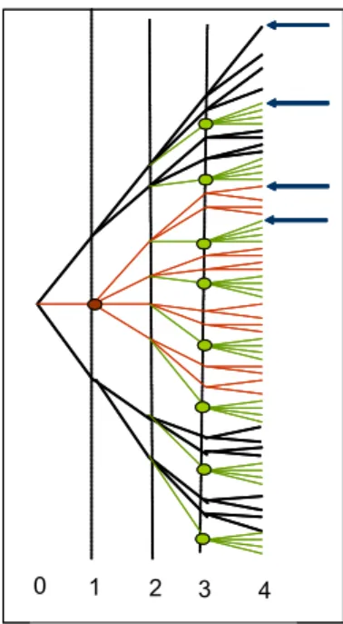
As a motivation to what follows, let us consider an example. Consider Tm = {0, 2, 4} and Tp = {1, 3} . At t = 1 there is a (1 − p) chance that
the stock price will not be observed. The same thing happens at t = 3. Hence, if there is no new information at these points in time, the σ-algebra describing the information available to the market will be Ft=Ft−1. In our
example, there are four different vectors y, given by y1 = (1, 1, 1, 1, 1) , y2 =
(1, 0, 1, 1, 1) , y3 = (1, 1, 1, 0, 1)and y4 = (1, 0, 1, 0, 1) .Each one is associated
with a given probability, respectively, p2, p (1− p) , p (1 − p) and (1 − p)2. We may describe the trees of information process associated to each of the four possible circumstances as follows
0 1 2 3 4 With probability p2 0 1 2 3 4 With probability p(1-p) 0 1 2 3 4 With probability p(1-p) 0 1 2 3 4 With probability (1-p)2 0 1 2 3 4 With probability p2 0 1 2 3 4 With probability p2 0 1 2 3 4 With probability p(1-p) 0 1 2 3 4 With probability p(1-p) 0 1 2 3 4 With probability p(1-p) 0 1 2 3 4 With probability (1-p)2
Figure 1: For each y the information available to the market can be repre-sented by a different tree.
The first tree (top, left) describes the case corresponding to vector y1,
where market exists at all points in time, coinciding with the perfectly liquid market tree. The second tree (top, right) reflects the second case, corre-sponding to vector y2, where market does not exist only at t = 1. We could
have drawn a tree with four branches going directly from the node at t = 0 to the corresponding four nodes at t = 2. We prefer the representation above, since we want to make clear that the filtration F1 reflecting the information
available at t = 1 is the same as the filtration F0 reflecting the information
available at t = 0. In a similar way we have a tree representing the vector y3 (low, left) and another one for the vector y4 (low, right). However, if we
want to describe all the possible situations in the same tree it will look like the one described below
This super-tree plays a main role in the construction of our superhedg-ing strategies. Actually, our extended filtration will work as if we have an extended tree, coinciding with the one above, where transactions would not be permitted at those nodes represented by open circles. We stress the point
0 1 2 3 4
0 1 2 3 4
Figure 2: This tree describes all the possibilities under probabilistic illiquidity at t = 1 and t = 3. The circles identify the nodes when it is not possible to transact. In the final nodes identified with arrows the stock price is the same.
that nodes in this tree do not represent mere price realizations. They are rather joint representations of the price process and the market existence process. For instance, the terminal nodes indicated with arrows in the figure are assumed to represent the same price level for the underlying asset, but with different market existence realizations.
We now focus on the construction of the superreplicating strategies in the case of probabilistic illiquidity. At any point in time, the number of shares and the amount invested in the risk-free asset will depend on the existence, or inexistence, of the market at the previous moments in time. However, these values will not depend on the future existence of the market.
Let ∆ (j, t; y) and B (j, t; y) denote, respectively, the number of shares and the amount invested in the risk free asset at node (j, t) for a given realization, y, of the process {ys}s∈T. We assume that, if yt = 0 and (j, t)
is an arbitrary successor of (i, t − 1) , then ∆ (j, t; y) = ∆ (i, t − 1; y) and B (j, t; y) = B (i, t− 1; y) , since the portfolio can not be rebalanced at time t. For any given two different sets y1 and y2 with common values y1
1 =
y2
1, y21 = y22, y31 = y32, . . . up to time t, we assume that
∆¡j, t; y1¢ = ∆¡j, t; y2¢ and B¡j, t; y1¢ = B¡j, t; y2¢.
Just as in the deterministic case, let V (j, t; y) denote the value process gen-erated by such portfolio [∆ (j, t; y) , B (j, t; y)], i.e.,
V (j, t; y) = ∆ (j, t; y) S (j, t) + B (j, t; y) Hence,
V ¡j, s; y1¢= V ¡j, s; y2¢.
In an analogous way to the case of probabilistic illiquidity the definition of self-financed strategy and superreplicating strategy is dependent on whether one is in a short or in a long position in the derivative.
In what follows we are going to characterize the upper and lower arbitrage-free bounds for the value of an American derivative in the case of probabilistic illiquidity.
4.2
Some Probabilistic Definitions
Analogously to what we did in section 2.1, we present some mathematical tools to obtain the arbitrage-free bounds of the American derivative.
We begin by defining Ty as the subset of points in T after the last
non-trading date. Formally we define Ty ={s ∈ T : s ≥ Θ (y)} with
Θ (y) = ½
0 if yt = 1,∀t ∈ T ,
Notice that for liquid markets Ty=T .
Definition 4.1 A node probability measure is a nonnegative function q (i, t; y), defined for any y and (i, t) with t ∈ Ty satisfying
X (j,t) X t∈Ty X yq (j, t; y) = 1. (16)
We now define a specific type of node probability measures.
Definition 4.2 A node probability measure on the event tree is said to be y-simple if, for each y, any t and t + k ∈ Ty, there are no two nodes in the
same path, say (i, t) and (j, t + k) ∈ i+t (t + k) , such that q (i, t; y) > 0 and
q (j, t + k; ˙y) > 0 where ˙y is any set such that y1 = ˙y1, . . . , yt= ˙yt.
The following theorem is analogous to theorem 2.1 but now in the frame-work of probabilistic illiquidity. Let Q (y) denote the set of all node proba-bility measures q (i, t; y).
Theorem 4.1 (Jha and Chalasani) The extreme points of the set of nodes Q (y) are simple node probability measures, i.e., on every path on the event tree there is at most one node where q is strictly positive.
The proof of this theorem follows closely the proof of theorem 2.1 and is presented in Appendix B.
Definition 4.3 An adjusted probability measure is a nonnegative func-tion p (i, t; y) defined for any y and (i, t) with t ∈ Ty such that p (0, 0) =
p (0, 0; y) = 1 and p (i, t; y) =X (j,s)∈i+t(s) X {z:z0=y0,... ,zt=yt} p (j, s; z) ,
with s = min {n ∈ Tz : yn= 1 and n > t} .
Let the set of all probability measures be denoted by Py. Also, let τy
denote an ordinary stopping time that is conditional on the realization of the process {yt}t∈T. For any y, τy is a map that is defined from Ω to
{s ∈ T : ys = 1} such that {w : τ (w; y) ≤ t} ∈ Ftfor all t ∈ {s ∈ T : ys= 1} .
Additionally, for two different sets y1 and y2 with common values y1
1 =
y2
1, y21 = y22, . . . , up to time t, if τ (w; y1) = tthen τ (w; y2) = t.We define a
nonnegative adapted process Xτ ,y associated with the stopping time that has
the form Xτ[i, k; y] = 1if τ (w; y) = k and Xτ[i, k; y] = 0otherwise. Let Ty
Definition 4.4 A y-simple node probability measure is said to be associated with a given stopping time if q (i, t; y) is equal to zero when Xτ(i, t; y) is
equal to zero, and q (i, t; y) is positive when Xτ(i, k; y) is strictly positive,
for any y and node (i, t).
Let the set of all node probability measures with this property be denoted by Qτ(y).
Definition 4.5 For any probability measure Py ∈ Py and stopping time τy ∈
Ty we say that Py is a τy-martingale measure if, Py-almost surely, for any
(i, t) and y such that yt= 1we have
X (j,s)∈i+(s) X s>t,s∈Tz X {z:z0=y0,... ,zt=yt} p (j, s; z) Xτ(j, s; z) £¯ S (i, t)− ¯S (j, s)¤= 0
The set of all Py that have this property is denoted by Py(τy)
Let (Py, Xτ ,y) denote a measure-strategy pair, i.e., a pair constituted by
an adjusted probability measure and a nonnegative adapted process.
Definition 4.6 A measure-strategy pair (Py, Xτ ,y) is said to be equivalent
to a node probability measure if, for any given node (i, t) with t ∈ Ty,
p (i, t; y) Xτ(i, t; y) = q (i, t; y) .
We can now enunciate the following result, adapted from Jha and Cha-lasani (2001) to include the random variable y.
Theorem 4.2 Consider a node probability measure q ∈ Q (y) . Then there exists a measure-strategy pair (Py, τy) equivalent to q, where for any given y,
Py is uniquely defined at node (i, t) where
q (i, t; y) + X (j,s)∈i+(s) X s>t,s∈Tz X {z:z0=y0,... ,zt=yt} q (j, s; z)
is strictly positive and, for a given y, τy is uniquely defined at nodes (i, t)
where q (i, t; y) is defined and is strictly positive. Conversely, if (Py, τy) is a
measure strategy-pair, then the node function q ∈ Q (y) such that q (i, t; y) = p (i, t; y) X (i, t; y) is the unique equivalent node-measure.
Proof. The proof of this theorem is a modification of the one provided in Jha and Chalasani (2001). See appendix.
All the mathematical definitions provided above are dependent of y. In what follows we will shown that it is possible to define an adjusted probability and a randomized stopping time in the original tree that is closely related with the concepts just presented.
Definition 4.7 An adjusted probability measure ¯P(i, t) is a nonnegative function such that ¯P (0, 0) = 1 and ¯P (i, t) = P(j,t+1)∈i+
t
¯
P (j, t + 1), for all t ∈ T .
The set of all probability measures ¯P is denoted by ¯P.
A randomized stopping time is a nonnegative adapted process X with the property that on every path of the event tree the sum of the random variable is equal to one, i.e.,
X
t∈T X (it, t) = 1 (17)
where it+1 ∈ i+t .The set of all randomized stopping time is denoted by X.
Definition 4.8 An adjusted probability measure ¯P ∈ ¯P is said to be a Xy
-martingale measure if there is a randomized stopping time X ∈ X, a stopping time τy ∈ Ty and an adjusted probability measure Py ∈ Py(τy) such
that
X (i, t) ¯P (i, t) =X
{y:yt=1}
p (i, t; y) Xτ(i, t; y)
for any (i, t) with t ∈ T .
The set of all ¯P that are Xy martingale measures is denoted by ¯P (Xy) .
Theorem 4.3 For any given τy-martingale measure, Py ∈ Py(τy) , the
ad-justed probability measure ¯P ∈ ¯P and the randomized stopping time X ∈ X such that ¯P is a Xy martingale measure are as follow. The adjusted
proba-bility measure is such that ¯P (0, 0) = 1 and for any (i, t)∈ jt−1+ (t) such that α (j, t− 1) 6= 0, where α (i, t) = X r≥t X {z:zt=1} p (i, r; z) Xτ(i, r; z) + X r≥s X (j,s)∈i+t−1 X {z:zt6=1} p (j, r; z) Xτ(j, r; z)
and s = min {r ∈ T : r > t and Xτ(j, r; z) = 1} then,
¯
P (i, t) = ¯P (j, t− 1)P α (i, t)
(i,t)∈jt+−1(t)α (i, t)
.
If P(i,t)∈j+
t−1(t)α (i, t) = 0 then ¯P (i, t) = ¯P (j, t− 1) for a given successor (i, t)
The randomized stopping time X ∈ X is uniquely defined for any node (i, t) such that ¯P (i, t)6= 0 and is given by
X (i, t) = P
{y:yt=1}p (i, t; y) Xτ(i, t; y)
¯
P (i, t) .
If ¯P (i, t) = 0 but there is a predecessor (k, t− 1) such that ¯P (k, t− 1) 6= 0 take X (i, t) = P (i,t)∈k+t−1(t)α (i, t) ¯ P (k, t− 1) . Otherwise, X (i, t) = 0.
Proof. See Appendix B3.
5
Results on Probabilistic Illiquidity
5.1
Upper bound for the Value of an American
Deriva-tive
The upper bound for the value of an American derivative is the maximum value for which the derivative would be transacted without allowing for ar-bitrage opportunities. As described in the deterministic illiquidity case, in order to find the upper bound consider a short position in the derivative. The maximum value for which the derivative would be transacted without allowing for arbitrage opportunities would be the value of the cheapest self-financed portfolio that the buyer of the derivative can buy in order to com-pletely hedge against any possibility of exercise of the American derivative.
A strategy is said to be a self-financed strategy if for any given y the portfolio at node (j, t1) , where t1 ∈ {t ∈ T : yt= 1} , generates in t2 a value
∆ (j, t1; y) S (i, t2) + B (j, t1; y) Rt2−t1 such that
∆ (j, t1; y) S (i, t2) + B (j, t1; y) Rt2−t1 ≥ V (i, t2; y) , (18)
with (i, t2)∈ jt+1(t2) and t2= min{s ∈ T : s > t and ys= 1} .
A sequence of portfolios {[∆ (j, t; y) , B (j, t; y)]}t∈T, one for each y, is said to be a superreplicating strategy if its value is higher than or equal to the payoff of the derivative at any node in the next transaction time. In other words, for any trading dates t1 and t2 such that t1 ∈ {t ∈ T : yt= 1} and
jt+1(t2) , the portfolio at t1, [∆ (j, t1; y) , B (j, t1; y)] , must be such as to
gen-erate in t2 a value ∆ (j, t1; y) S (i, t2) + B (j, t1; y) Rt2−t1 such that
∆ (j, t1; y) S (i, t2) + B (j, t1; y) Rt2−t1 ≥ G (i, t2) . (19)
Since it is the cheapest initial portfolio, the upper bound Vu
p must satisfy
Vpu = min V (0, 0).
The decision variables are the ∆ (j, t; y) and B (j, t; y) for all non-terminal nodes of the event tree. However, this optimization is subject to the con-straints of self-financing (18) and superreplication (19).
More formally, for any given y take any t1 ∈ T such that yt1 = 1. Define
the consecutive trading date t2such that t2 = min (s∈ T : s > t1 and ys = 1) .
The upper bound for the value of the American derivative can thus be seen as the solution of the following problem:
Vpu = min
{∆(j,t;y),B(j,t;y)}t∈{s∈T :ys=1}\{T }
∆ (0, 0) S (0, 0) + B (0, 0)
subject to the superreplicating restrictions:
∆ (0, 0) S (0, 0) + B (0, 0)≥ G (0, 0) , (20)
∆ (j, t1; y) S (i, t2) + B (j, t1; y) Rt2−t1 ≥ G (i, t2) , (21)
and subject to the self-financing restrictions:
∆ (j, t1; y) S (i, t2) + B (j, t1; y) Rt2−t1 ≥ ∆ (i, t2; y) S (i, t2) + B (i, t2; y)
(22) for any (i, t2)∈ jt+1(t2) .
Using results from linear programming the upper bound arbitrage free bound of the American derivative can be written as follows.
Theorem 5.1 There is a node probability measure q ∈ Q (y) such that the upper hedging price of an American derivative in a probabilistic dry market can be written as Vpu = max q∈Q(y) X (j,t) X t∈Ty X yq (j, t; y) ¯G (j, t) with X (j,s)∈i+t(s) X s>t,s∈Tz X {z:z0=y0,... ,zt=yt} p (j, s; z) Xτ(j, s; z) £¯ S (i, t)− ¯S (j, s)¤= 0
Proof. This proof follows the methodology used in theorem (3.2). As the upper bound for the value of the American derivative, Vu
p , is the solution of
linear programming problem it is possible to construct its dual. Let λ (0, 0) , λ (i, t2; y) and γ (i, t2; y) denote the dual variables that are associated,
re-spectively, with the restrictions (20), (21) and (22) of the primal problem. Note that, as we assume that given two different sets y1 and y2 with common values y1
1 = y12, y12 = y22, y31 = y23, . . . up to time t1, the portfolio will be the
same, i.e., ∆¡j, t1; y1 ¢ = ∆¡j, t1; y2 ¢ and B¡j, t1; y1 ¢ = B¡j, t1; y2 ¢ ,
then, λ (i, t2; y1) = λ (i, t2; y2) for all (i, t2) ∈ i+t1(t2) . Before presenting the
dual problem let define
Θt={y :yt = 1 and min [s ∈ Ty : s > t] = min [s∈ T : ys = 1 and s > t]} .
The dual problem is given by
max q∈Q(y) X (j,t) X t∈Ty X yλ (j, t; y) ¯G (j, t)
subject to the conditions: λ (0, 0) S (0, 0) +X (j,s)∈i+0(t) X z∈Θ0 [λ (j, t; z) + γ (j, t; z)] S (j, t) = S (0, 0) , (23) λ (0, 0) +X (j,s)∈i+0(t) X z∈Θ0 [λ (j, t; z) + γ (j, t; z)] Rt = 1 (24) where t = min {s ∈ Tz : s > 0}.
For any (i, t) and y such that t ∈ Ty\ {0, max [r ∈ Ty and r < T ] , T } ,
X (j,s)∈i+t (s) X z∈Θt [λ (j, s; z) + γ (j, s; z)] S (j, s) = γ (i, t; y) S (i, t) (25) and X (j,s)∈i+t(s) X z∈Θt [λ (j, s; z) + γ (j, s; z)] Rs−t = γ (i, t; y) (26)
where s = min {r ∈ Tz : r > t} . Finally, for any (i, t) and y such that t =
max{r ∈ Ty and r < T } X (j,T )∈i+t(T ) X z∈Θt λ (j, T ; z) S (j, T )− γ (i, t; y) S (i, t) = 0 (27)
and X (j,T )∈i+t(T ) X z∈Θt λ (j, T ; z) RT −t− γ (i, t; y) = 0 (28)
The restrictions presented in equations (25) and (27) can be rewritten as S (i, t) γ (i, t) = X r≥s X (j,r)∈i+t (r) X z∈Θt λ (j, r; z) S (j, r)
and the restrictions presented in equations (26) and (28) can be rewritten as γ (i, t) =X r≥s X (j,s)∈i+t(s) X z∈Θt λ (j, r; z) Rr−t.
for all (i, t), t ∈ T \ {0, T } and with s = min {r ∈ Tz : r > t} . The two
pre-vious equations can be written as S (i, t)X r≥s X (j,s)∈i+t(s) X z∈Θt λ (j, r; z) Rr−t = X r≥s X (j,s)∈i+t(s) X z∈Θt λ (j, r; z) S (j, r)
Taking into account equations (23) and (24) we obtain, for all t ∈ T \ {T } S (i, t)X r≥s X (j,s)∈i+t(s) X z∈Θt λ (j, r; z) Rr−t = X r≥s X (j,s)∈i+t(s) X z∈Θt λ (j, r; z) S (j, r) with X t∈Ty X (j,t) X yλ (j, t; y) R t = 1.
Let q (i, t; y) = λ (i, t; y) Rt.then, ¯ S (i, t)X r≥s X (j,s)∈i+t(s) X z∈Θt λ (j, r; z) Rr−t = X r≥s X (j,s)∈i+t(s) X z∈Θt λ (j, r; z) ¯S (j, r) and X t∈Ty X (j,t) X yq (j, t; y) = 1.
The upper bound solving the problem above can also be seen as the solution of a more intuitive problem. In fact, it can be shown that this upper bound maximizes over all possible stopping times the expected discounted payoff, when the expectation is optimized among all adjusted probability measures. In other words,
Theorem 5.2 There is an adjusted probability measure Py ∈ Py(τy) and an
adapted process Xτ ,y ∈ XT,y such that the upper hedging price of an American
derivative in a probabilistic dry market can be written as Vpu = max
Xτ ,y∈XT,y
max
Py∈Py(τy)
Ep¯GXτ ,y
where GXτ ,y(i, t) = G (i, t) Xτ ,y(i, t)
Proof. In an analogous way to the proof of theorem (3.2), using theorem (4.1) and theorem (4.2) the conclusion is straightforward.
Note that this result is the same that would be obtained if the filtration that describes the stock price is an augmented one, in the spirit of the one presented in figure (2), with no uncertainty about the existence of the market and no transactions in some nodes (the ones identified in the figure).
However, the upper bound of the value of an American derivative can also be written using randomized stopping times if an adjusted probability measure with an additional characteristic is considered. The adjusted prob-ability measure have to be decomposed in such a way that if an augmented filtration is considered the stock price is a martingale.
If the initial filtration is considered it is not possible to write the upper bound as an optimization over ordinary stopping times, as in theorem (5.2). In this case, randomized stopping times may be needed.
Theorem 5.3 There is an adjusted probability measure ¯P ∈ ¯P (Xy) and a
process X ∈ X such that the upper hedging price of an American derivative in a probabilistic dry market can be written as
Vpu = max
X∈XP ∈ ¯¯maxP(Xy)E ¯ pG
X
with GX(i, t) = G (i, t) X (i, t) .
Proof. This result follows from the application of theorem (4.3) to the result presented in theorem (5.2).
In what follows we are going to consider an example. The upper bound of the American derivative is obtained using the primal and the dual problem. In this example no optimal pure stopping time exists that maximizes the expected value of the payoffs of the American derivative. The expected value of the payoffs of the American derivative is maximized with randomized stopping times.
Consider T = {0, 1, 2} , T = {0, 2} and Tp = {1} . Let R = 1 and the
uncertainty about the price of the underlying stock and the derivative be given by
S0=3 G0=0 S1=2 G1=5 S2=4 G2=8 S0=3 G0=0 S1=2 G1=5 S2=4 G2=8 Figure 3:
There are two sets y, y1 = {1, 1, 1} and y2 = {1, 0, 1} . The optimum
value of the variables in the primal problem is
∆ (0, 0; y1) = ∆ (0, 0; y2) = ∆ (0, 0) = 1, 5
B (0, 0; y1) = B (0, 0; y2) = B (0, 0) = 2
∆ (0, 1; y1) = 2, 5
B (0, 1; y1) = 0
that results in an optimum value of the function ∆ (0, 0) S (0, 0) + B (0, 0) = 6, 5.
In what concerns the dual problem the optimum value of the variables q (0, 0) = q (0, 0; y1) = q (0, 0; y2) = 0
q (0, 1) = q (0, 1; y1) = 0.5
q (0, 2) = q (0, 2; y1) + q (0, 2; y2) = 0 + 0.5 = 0.5
As a result, the optimum value of the objective function is q (0, 1) G (0, 1) + q (0, 2) G (0, 2) = 6.5. In this case the probability measure Py is given by
py(0, 0) = 1
py(0, 1, y1) = 1∗ 0.5+0.50.5 = 0.5
py(0, 2, y1) = 0.5
py(0, 2, y2) = 0.5
and the stopping time τy is such that Xτ is given by
Xτ(0, 0) = 0
Xτ(0, 1, y1) = 1
Xτ(0, 1, y2) = 0
Xτ(0, 2, y1) = 0
The probability measure ¯P is
P (0, 0) = P (0, 1) = P (0, 2) = 1 and the randomized stopping time X
X (0, 0) = 0 X (0, 1) = 0.5 X (0, 2) = 0.5
The use of the randomized stopping times is closed related to the fact that we are using the filtration that reflects the information that is available if the market is completely liquid.
5.2
Lower bound for the Value of an American
Deriva-tive
The lower bound for the value of an American derivative is the minimum value for which the derivative would be transacted without allowing for ar-bitrage opportunities. As in the deterministic illiquidity case, in order to find the lower bound consider a long position in the derivative. For a given exercise policy consider the most expensive self-financed portfolio that the buyer of the American derivative can buy in order to be fully hedged. The minimum value for which the derivative would be transacted without allow-ing for arbitrage opportunities would be the value of most expensive portfolio chosen among all the portfolios just mentioned.
For any given exercise policy τy and any node (j, t), such that (j, t) is
before the exercise time, consider the portfolio constituted of ∆τy(j, t; y)
shares of the underlying asset and an amount Bτy(j, t; y)invested in the risk
free asset. Its value process is given by
Vτy(i, t
2; y) = ∆τy(i, t2; y) S (i, t2) + Bτy(i, t2; y)
For a long position in the derivative, a strategy is said to be a self-financed strategy if for an any given y the portfolio at node (j, t1) , where t1 ∈
{t ∈ T : yt = 1} , generates in t2 a value such that
∆τy(j, t
1; y) S (i, t2) + Bτy(j, t1; y) Rt2−t1 ≤ Vτy(i, t2; y) , (29)
with (i, t2)∈ jt+1(t2), t2= min{s ∈ T : s > t and ys = 1} such that there is a
A sequence of portfolios {[∆τy(j, t; y) , Bτy(j, t; y)]}
t∈T, one for each y, is
said to be a superreplicating strategy if its value is higher than or equal to the payoff of the derivative at any node in the next transaction time. In other words, for any trading dates t1 and t2 such that t1 ∈ {t ∈ T : yt= 1} and
t2= min{t ∈ T : t > t1 and yt= 1} and arbitrary nodes, (j, t1) and (i, t2) ∈
jt+1(t2)such that Xτ(i, t2) = 1,the portfolio at t1, [∆
τ(j, t
1; y) , Bτ(j, t1; y)] ,
must be such as to generate in t2 a value such that
∆τy(j, t
1; y) S (i, t2) + Bτy(j, t1; y) Rt2−t1 ≤ Gτy(i, t2) . (30)
As described above, this would be the value of the most expensive self-financing, ”superreplicating” portfolio. Since it is the most expensive initial portfolio, the upper bound Vu must satisfy
Vpl = max
τy
Vτy(0, 0).
The decision variables are the ∆τ(j, t; y)and Bτ(j, t; y) for all non-terminal
nodes of the event tree. However, this optimization is subject to the con-straints of self-financing (29) and superreplication (30).
More formally, for any given y take any t1 ∈ T such that yt1 = 1. Define
the consecutive trading date as t2 = min (s∈ T : s > t1 and ys = 1) . The
lower bound for the value of the American derivative can thus be seen as the solution of the following problem:
Vpl = max τy∈Ty
max
{∆(j,t;y),B(j,t;y)}t∈{s∈T :ys=1}\{T }
∆τy(0, 0) S (0, 0) + Bτy(0, 0)
subject to the superreplicating restriction ∆τy(0, 0) S (0, 0) + Bτy(0, 0)
≤ Gτ(0, 0) ,
if Xτy(0, 0) = 1. However, if Xτy(0, 0) = 0, the superreplication condition is
defined for any node (i, t2) such that X (i, t2) = 1, and is given by
∆τy(j, t
1) S (i, t2) + Bτy(j, t1) Rt2−t1 ≤ Gτy(i, t2) ,
for any t1 ∈ Tm\ {T } such that (i, t2)∈ j+(t2)and t2 = min (s∈ Tm : s > t1) .
Additionally, for any node (i, t2)such that Xτy(i, t2) = 1the self-financing
conditions apply, i.e., ∆τy(k, t
1) Sτy(i, t2) + Bτy(k, t1) Rt2−t1 ≤ ∆τy(i, t2) S (i, t2) + Bτy(i, t2)
for all t1 ∈ Tm\ {max {t ∈ Tm : t < T} , T } and (i, t2) ∈ j+(t2) with t2 =
min (s ∈ Tm\ {T } : s > t1) .
Using results from linear programming the upper bound arbitrage free bound of the American derivative can be written as follows.
Theorem 5.4 There is a node probability measure q ∈ Qτ(y) and a process
τy ∈ Ty such that the upper hedging price of an American derivative in a
probabilistic dry market can be written as
Vpl= max τy∈Ty min q∈Qτ(y) X (j,t) X t∈Ty X yq (j, t; y) ¯Gτy(j, t)
such that for any (i, t)and t ∈ T X
m>t,m∈Tm
X
(j,m)∈i+t(m)
q (j, m)£S (i, t)¯ − ¯S (j, m)¤= 0.
Proof. For a given stopping time the problem that must be solved in order to find the lower bound for the value of the American derivative can be rewritten as Vpl= min q∈Qτ(y) X (j,t) X t∈Ty X yq (j, t; y) ¯Gτy(j, t)
such that for any (i, t)and t ∈ Tm
X
m>t,m∈Tm
X
(j,m)∈i+t(m)
q (j, m)£S (i, t)¯ − ¯S (j, m)¤= 0.
Considering the optimization with respect to τy the problem becomes
max τy∈Ty min q∈Qτ X (j,t) X t∈Ty X yq (j, t; y) ¯Gτy(j, t)
such that for any (i, t) with t ∈ T X
m>t,m∈Tm
X
(j,m)∈i+t(m)
q (j, m)£S (i, t)¯ − ¯S (j, m)¤= 0.
Theorem 5.5 There is an adjusted probability measure ¯P ∈ ¯P (Xy) and a
process τy ∈ Ty such that the lower hedging price of an American derivative
in a probabilistic dry market can be written as Vpl= max τy∈Ty min ¯ P ∈ ¯P(Xy) EpGτy
Proof. Using the result presented in theorem (5.4) and the theorem (4.2) the proof is straightforward.
If the stopping times are defined in the original filtration, i.e., in the filtration F = F0, F1, . . . , FT, where Ft= σ (St) then randomized stopping
times have to be considered.
Theorem 5.6 There is an adjusted probability measure ¯P ∈ ¯P (Xy) and a
process X ∈ X such that the lower hedging price of an American derivative in a probabilistic dry market can be written as
Vpu = max
X∈XP ∈ ¯¯maxP(Xy)E ¯ pG
X
with GX(i, t) = G (i, t) X (i, t) .
Proof. This result follows from the application of theorem (4.3) to the result presented in theorem (5.5).
6
Comparison of the Results
In this section we will compare the arbitrage-free bounds of an American derivative in a deterministic dry market, in a probabilistic dry market and in a market where transactions are possible at any point in time. In other words, we will compare the arbitrage-free bounds of an American derivative if, at some given points in time, transactions are not possible, transactions are possible with a given probability and transactions are possible.
The upper bound in a probabilistic dry market is higher than or equal to the upper bound if the market is dry in the deterministic sense. Moreover, it is also equal to or higher than the upper bound if transactions were possible at all points in time. The reason is that we are using the pure arbitrage-free concept. If, at a given point in time, it becomes possible to transact with a given probability, the seller of the American derivative must hedge against the possibility of exercise at that point in time. The value of the probability is irrelevant because he will hedge against the worse scenario. In what concerns the upper bound in a deterministic dry market it can be smaller or higher than the upper bound if transactions were possible at all points in time. The reason for this is quite intuitive. Consider an American derivative with a very high payoff in a given moment where transactions were not possible due to the deterministic dryness. If transactions were possible at that given moment in time, the value of the American derivative could increase to become higher than the upper bound in a deterministic dry market.
The lower bound in a probabilistic dry market is higher than or equal to the lower bound if the market is dry in the deterministic sense and is equal to the lower bound if transactions were possible at all points in time (Vl). In what concerns the comparison with the deterministic case note that the problem that must solved to obtain the lower bound in the deterministic case is a ”subset” of the problem that is solved to find the lower bound in the probabilistic case. It corresponds to the y with the highest number of components equal to zero. Hence, Vl
p ≥ Vdl.On the other hand, the problem
that must solved to obtain the lower bound in the case where transactions are possible at all points in time is also a ”subset” of the problem that is solved to find the lower bound in the probabilistic case. It corresponds to the y with all components equal to one. Hence, Vpl ≥ Vl. Moreover, in the
probabilistic case, the trading strategies that solve the problem for any y whose components are not all equal to one is a possible solution when y has all components equal to one. Therefore, we can conclude that Vpl = Vl.
Considering that the only source of incompleteness in the market is the non-existence, or the possibility of non-existence, of the market at some points in time if transactions if transactions were possible at all points in time, markets would be complete and there would be a unique arbitrage-free value for any American derivative. We found out that this unique arbitrage-free value for each American derivative is equal to the lower bound of the arbitrage-free range of variation for its value under a probabilistic dry market. However, it may not belong to the arbitrage-free range if a deterministic dry market is considered.
If the market is incomplete even with the existence of transactions at all points in time it is not possible to find a unique arbitrage free value for the American derivative. However, it is also possible to establish an arbitrage free range of variation for the value of the American derivative. This range will be a subset of the arbitrage free range of variation for the value of the American derivative in the case of probabilistic dryness, but may be wider than the arbitrage free range of variation in the deterministic case.
7
Exercise Policy
In order to understand the optimal exercise policy, we start presenting the case of a complete market. In this case, the value of an American derivative is given by
Vu = max
τ ∈T maxP ∈P E pG
τ (31)
If the solution is unique, the stopping time that solves (31) is the opti-mal exercise policy for the holder of the American derivative. The reason is as follows. Given an optimal stopping time τ∗, we may define a stopping time frontier as the set of nodes (i, t) such that Xτ∗(i, t) = 1. Recalling
that there is an optimal stopping node for each possible path2, we define
the interior of the stopping time frontier as the set of predecessors of the nodes that constitute the frontier. It follows that no rational agent exercises the American derivative at a node inside the stopping time frontier, because at such nodes, the American derivative is worth more than the correspond-ing exercise. Whenever the stoppcorrespond-ing time frontier is reached, the American derivative will be exercised by a rational agent. This happens because the derivative’s payoff at that point is larger than the cost of a replicating port-folio, guaranteeing the derivative’s payoff in the future.
If the solution is not unique there may be indeterminacy. An example illustrates this point. Consider the non-terminal node (i, t1)and the terminal
nodes (j, t2) and (m, t2), which are the immediate successors of (i, t1) . The
replicating portfolio, at node (i, t1) , is the pair [∆ (i, t1) , B (i, t1)]. Assume
that this portfolio satisfies
∆ (i, t1) S (j, t2) + B (i, t1) R = G (j, t2)
∆ (i, t1) S (m, t2) + B (i, t1) R = G (m, t2)
(32)
We also assume that, at node (i, t1) ,
G (i, t1) = V (i, t1) . (33)
In this case, the value of the portfolio, at node (i, t1), that replicates the value
of the American derivative in nodes (j, t2)and (m, t2)is the same as the payoff
of the American derivative. Let P (i, t1) denote the price of the American
derivative at node (i, t1) . In this case P (i, t1) = G (i, t1) = V (i, t1) . Hence,
the holder of the American derivative will obtain the same payoff exercising or selling the derivative.
In what concerns the dual variables, if, in the primal problem, the repli-cating portfolio satisfies 32 and 33 the solution of the dual problem is not unique. There are several node probability measures q solving the maximiza-tion problem that characterizes the upper bound. Let q1 and q2 denote two
possible solutions. In that case q1 and q2 must satisfy
Vu = max
q1∈Q
X
(i,t)∈Jt
t∈Tm
q1(i, t) ¯G (i, t) = max q2∈Q
X
(i,t)∈Jt
t∈Tm
q2(i, t) ¯G (i, t)
2If the solution is unique, there is a unique strictly positive q associated to each path.