1
1
Fevereiro de 2016
Working
Paper
414
Cash-cum-in-kind transfers and income tax
function
TEXTO PARA DISCUSSÃO 414•FEVEREIRO DE 2016• 1
Os artigos dos Textos para Discussão da Escola de Economia de São Paulo da Fundação Getulio
Vargas são de inteira responsabilidade dos autores e não refletem necessariamente a opinião da
FGV-EESP. É permitida a reprodução total ou parcial dos artigos, desde que creditada a fonte.
Cash-cum-in-kind transfers and income tax function
Enlinson Mattos
∗Rafael Terra
†April 12, 2013
Abstract
This paper investigates income tax revenues response to tax rate changes taking into consideration that cash-cum-in-kind transfers are used as a redistributive package to the community. First, we show that when cash and in-kind transfers are not tied to be substitute instruments, a marginal income tax increase mayunambiguouslydecrease the quantity supplied of labor (and tax revenues therein). Next, we show that whenever the government chooses the optimum provision for the publicly provided good the tax revenue function has a negatively-sloped part with respect to tax rates except for one case. Last, we consider Brazilian data - PNAD - from 1976 to 2008 to test our theoretical implications. Our estimations suggest a weak evidence in favor of the existence of a Laffer-type curve for Brazilian income tax revenues data. Moreover, we find that the actual average income tax rate seems to be below the estimated optimum level. In a shorter sample from 1996-1999, we find evidence that labor supply decreases with tax rate when cash and in-kind transfers are in play. Using a pseudo-panel from the same shorter sample, we try to estimate the elasticity of taxable income, following Creedy and Gemmell (2012) and Saez et al. (2009). We explore a small tax reform between 1997 and 1998 that affected only the higher income tax bracket, and find evidence that Brazil is on the revenue reducing side of the Laffer Curve, at least for individuals in the higher income tax bracket.
JEL classification: H42, H31, H21, H23.
Keywords: Labor supply, tax rates and cash-cum-in-kind transfers.
1
Introduction
In any modern economy, governments rely on both cash and in kind transfers to their community. Examples of such policies are all abound. While pension funds (most expressive) and pro-poor redistributive programs such as EITC in U.S. and many conditional cash transfers (CCT) in developing economies are examples of cash transfers, public education, health and housing can be considered representatives of in-kind transfers for many countries. The literature usually points out cash transfer as the preferred mechanism for redistribution because it does not constraint the behavior of the individuals. Nevertheless, Curry and Gahvari (2007) stress that the share of in-kind transfers are increasing over time in many countries. The authors argue many reasons for that to occur. This includes the role played by in-kind transfers by facilitating self-targeting in a imperfect information setting (Besley and Coate, 1991; Gahvari and Mattos, 2007) as well as the possibility to improve tax efficiency because it could increase labor supply reduced previously by the substitution effect due to the imposition of a linear tax (Murray, 1980; Leonesio, 1988; and Gahvari, 1994) or non-linear tax (Munro, 1992; Blomquist and Christiansen, 1998; Boadway and Marchand, 1995; Cremer and Gahvari, 1997 and Creedy et al, 2008).
This paper attempts to investigate the role played by government expenditures on the determination of tax revenues, but focusing on the role played by cash-cum-in-kind transfers on labor supply and consequently on tax revenues. The main contribution of this paper relies on providing a theoretical motivation for the existence of a Laffer curve in income tax revenue under cash-cum-in-kind transfers followed by an empirical investigation of some of the implications of the model. Therefore, we first characterize the conditions of a negatively relation between tax revenue and tax rate when governments rely on cash-cum-in-kind trans-fers. These transfers are widely used in practice and justify the investigation of tax revenue function under this set up. Second, we also bring empirical evidence for Brazil, a developing country that relies heavily on cash transfers as a redistributive policy. That is reinforced by the more recent redistributive policies adopted in that country, one of the leading countries in terms of implementation of conditional cash transfers.
revenue function with the nature of the governments. In particular the author demonstrates that whenever the government decides to provide in-kind transfers (instead of cash), such discontinuity appears and one can no longer verify a negatively sloped tax function. 1 Only
recently Chang and Peng (2012) explores the conditions of the existence of a Laffer curve for income and consumption taxes. They find that if all goods are weak gross substitutes, then a Laffer type relationship between consumption taxes and tax revenues exists, and the Marginal Cost of Public Funds (MCF) is high. If all goods are weak gross complements, then the labor is provided inelastically and such relationship does not exist, and it could be possible to increase tax revenue raising consumption taxes indefinitely. 2
When income tax is the variable of interest, labor supply assumes the central role of tax basis. Therefore this paper is also related to debate about labor supply response to income tax changes. This debate is centralized in the general equilibrium effects on the labor supply. For instance Hausman (1981), presents a standard income-leisure analysis to make the point clear: lower tax rates increases the net wage that can be earned from an additional hour of work (substitution effect), but also can keep the same standard of living with less work (income effect). However, Gwartney and Stroup (1983) and Ehrenberg and Smith (1985) point out that this analysis does not take the aggregated labor market into consideration. The authors argue that a tax cut does not increase aggregate real income by the amount of the tax reduction, i.e., it does not change the technical production possibilities of the economy. In their general equilibrium model, a tax cut will generate a decline in the public goods expenditures which in turn, will offset the expansion in private goods expenses. That eliminates the income effect, leaving the unambiguously positive (substitution) effect of tax cut on labor supply. On the other hand, Gahvari (1986) argues that this latter claim only would be correct if the tax revenues are handed back to individuals as cash transfers and both private and public goods can be bought freely in the market. The author explains that in the case that a tax cut causes a reduction in the provision of the public good, then indi-viduals face a constrained market, which in turn forces them to consume different bundles than the ones they would choose if they received the value in cash.3
1
See Wilson (1991a and 1991b) for optimal provision of public goods and Atkinson and Stern (1974) for marginal cost of public funds and provision of a public good.
2
The argument for a possible bell-shaped relationship between tax revenue and tax rate seems to be popularized by Arthur Laffer in 1974. The basics of this idea constitute that change in tax rates has two effects: one labeled as arithmetic and the other is economic. The first is simply a direct change on tax revenue due to tax change. The second effect recognizes the change in behavior of agents involved when there is such tax change which, in turn, could affect tax basis. Therefore the final effect is composed by these two effects aggregated. The Laffer curve characterizes such trade-off suggesting that tax revenue would go to zero as tax rate goes to one. This idea has been very contested in the literature as discussed previously. See also Buchanan and Lee (1982) for a more general perspective of this curve.
3
Nevertheless, our model shows, first, that if in-kind transfers and leisure are Hicks sub-stitutes (complements), leisure is normal, and in-kind transfer can be ‘topped up’ or is (over)under provided- a marginal income tax raises unambiguously (in)decreases the quan-tity supplied of labor if there is a concomitant (in)decrease in the public good provision. Next, restricting to optimum public provision of the private good, we show that whenever the extent of normality for leisure is bounded we may also observe negative relationship between income tax revenue and tax rates.
Moving to empirical evidence, the (vast) literature on labor supply and taxation ignores the effect of public expenditures and concentrates on the precise estimate of tax reform on the labor market (Meghir and Phillips, 2008). The conclusion of this is that hours of work are relatively inelastic for men, but are a bit more responsive for married women and single mothers. Participation is sensitive to taxation and benefits only for women and less educated men. Conway (1997) and Duarte et al (2011) seem to be the only exceptions that address individual labor supply response taking into consideration aggregated public expenditures provided. Both show that in-kind transfers affect labor supply directly and also the coefficient of tax rate (tax rate labor response). Duarte et al (2011) find also that the combination of cash versus in-kind transfers do affect labor supply. They argue that such general equilibrium perspective should be taken into consideration, since its omission could drive to biased estimation of tax rate response on the part of labor supply.
More related to our perspective, there are some papers that attempt to estimate in a more direct manner the income tax revenue as function of tax rates, focusing on the possibility of a bell shaped version of that function, the Laffer curve. Fullerton (1982), Feige and McGee (1982), Lyndsey (1987), Van Ravestein and Vijbrief (1988) and Heijman and Van Ophem (2005) look for the optimum tax rate, i.e., they look for the tax rate level that maximizes revenues. They find actual tax rates were more than the optimum in Sweden (Stuart, 1981), less than the optimum in Netherlands (Van Ravestein and Vijbrief, 1988) and inconclusive for United States (Fullerton, 1982 and Lindsey, 1987).4 Recently, Trabandt and Uhlig (2011)
simulate the Laffer Curve for United States and aggregated European Union. The authors find that the revenues in the US of either labor or capital income taxation can be increased by
public provision of a good under non-linear income taxation. This literature addresses two types of provision. First, when only the poor can consume the publicly provided good (Blomquist and Christiansen, 1995, 1998) while the second follows Gahvari (1995) and addresses a universal public provision policy.
4
respectively 30% and 6% by the increase of the tax rates, i.e. taxes are to the left of Laffer’s Curve peak. For the EU countries the labor and capital income taxes can be increased by only 8% and 1%, respectively. Consumption tax revenue function does not show a Laffer curve format, it is everywhere increasing.
Our empirical approach constitutes of two strategies. We first want to check whether income tax function in Brazil can be modeled as a bell-shaped function with respect to income tax rates in a more direct manner. To a certain extent, this approach is similar to Hsing (1996) because we consider a time series data set from 1977 to 2008, at the national level. From this data we can identify the municipalities individuals live in only for 1996 to 1999. Therefore, for this subsample, we first calculate the income tax collected from each individual and aggregated within the municipality forming a panel of 817 municipalities that goes from 1996 to 1999. This strategy allows us to identify the correspondent portion of public expenditures assigned to the representative consumer in that municipality. Then we estimate labor supply response to tax rates controlling for cash and in-kind transfers. Last, we estimate tax revenue response for the representative consumer of these municipalities in order to compare to our aggregated result.
Our empirical estimations show evidence that such bell-shaped curve might represent income tax revenue function for Brazil during 1977 to 2008. Although we find the correct coefficients and statistical significance for a concave function, some specifications with all variables in differences and in the logarithmic scale do no present statistically significant coefficients (even though most of the models present coefficients with the correct signs). Also, using a panel of 817 municipalities for the period 1996-1999 we find that labor supply is affected by cash transfers differently than its counterpart in-kind transfers. Moreover, we find a negative relation between tax rates and labor supply reinforcing the possibility of a Laffer curve.
The paper is divided as follows. Next section describes our model and derive its implica-tion. Section 3 addresses the empirical issues involved while bringing theory to the data and presents our empirical strategy. Section 4 brings our estimation results. Section 5 concludes.
2
The model
preferences for the consumers can be represented by the utility funciton u(x, l, g). Assume
u(.) is quasi-concave and twice differentiable function in all its arguments. Assume further that (i) ui/uj →0 if and only if j → ∞ and (ii)ui/uj → ∞ if and only if j →0. These
as-sumptions guarantee that the marginal rate of substitution betweeniandj is always defined for positive i and j and rule out discontinuous at a tax rate lower than one. The markets are assumed to be competitive and as in Gwartney and Stroup (1983) and Gahvari (1986, 1989), that both goods are produced using only laborL. We also assume linear production functions:
nx =AnLx (1)
ng=BnLg (2)
where A and B are constants and Lx and Lg denotes the labor supply dedicated to the
provision of goods x and g respectively. It is important to point that linear technologies assumed here guarantees the relative prices of x, g and l are fixed. We also rule out many general equilibrium problems addressed in Malconson (1986) when verifying the shape of tax revenue function. 5
Both goods x and g are produced in the market. But the last one is financed through a linear income tax θ combined with a cash transfer, s6. The lump-sum transfer can be positive (tax) or negative (rebate) and is provided to all individuals as long as they consume the public good.7 The income tax revenue function of the government can be written as
R(θ) =nθw(1−l) = npg+ns. (3) where p is the production price of g, npg is the aggregated expenditure on the publicly provided good and each individual’s leisure endowment is set equal to 1, i.e.,Lx+Lg+l = 1.
Now differentiating R(θ) totally with respect to θ,
dR(θ)
dθ =nw(1−l)−θnw dl
dθ (4)
5
Although most of the results could be extended using diminishing returns to scale prodution functions, that would distract from our purpose here, which is to determine the role played by cash-cum-in-kind transfers.
6
This paper differentiates from Gahvari (1990) because both instruments s and g are allowed to be complementary and not only substitutes in order to compensate variations inθ.
7
It is plain that a necessary condition for a negative slope of R(θ) above is that dl/dθ >
0. That condition is investigated below. A more difficult question regards the sufficient condition for havingR(θ) a negatively sloped piece for 0< θ <1. this can be shown using an alternative version of the Rolle’s theorem.8 This alternative version of the theorem requires
that (i) R(θ) to be continuous in the interval (0,1), (ii) R(0) = 0 and (iii) limθ→1R(θ) =
0, and the domain for R(.) is the interval [0,1).9 We explore this issue in the following
subsection.
3
The role played by cash-cum-in-kind Transfers
3.1
Necessary condition for a negatively-sloped tax function
The consumer treats s as fixed and maximize utility subject to a given g = g and the budget constraint,
x=w(1−θ)(1−l) +s (5) The first order condition can be written as10
ul
ux
=w(1−θ) (6)
where subscripts of u denote partial derivatives. Both equations 5 and 6 determine the demand functions l = l(p, g, w(1− θ), s) and x = x(p, g, w(1−θ), s). Substituting these functions into the utility function gives,
u∗
=v(w(1−θ), g, s) =u(x(g, w(1−θ), s), l(g, w(1−θ), s), g) (7)
The following definition is important at this stage,
8
A similar approach has been used in Gahvari (1989).
9
This leads to another simplification since we avoid the case thatR(1) becomes a correspondence rather a function for some utility function. Another advantage of this alternative version is that R(θ) is required to be continuous only in the open interval (0,1) so one can ignore whether or not ui/uj is defined for i or
j= 0.
10
Definition 1 Good g is said to be provided at the first best level if, in comparison to his current position, the transfer recipient is indifferent between an offer of one dollar cut (raise) in his amount of in-kind transfers, coupled with a one dollar increase (decrease) in his cash grants. Formally, g is provided at the first level whenever [∂v/∂g]/[∂v/∂s] =p.
Note that the first best level for g can be easily reached when the individuals decide how much to consume of that particular good, i.e.,ug/ux =p. Further, assume that 0≤θ ≤1.11
Now, note then that the compensated (constrained) demand for leisure, lc may be derived
from the dual to the constrained utility maximization and by definition,
l(g, w(1−θ), s)≡lc(g, w(1−θ), v(w(1−θ), g, s)) (8)
For later reference it is useful to present the following result derived in Gahvari (1994) (see his Lemma 1, p. 499).
Lemma 2 If g and l are Hicks substitutes (complementaries), then ∂lc/∂g <(>)0.
Our first proposition summarizes the necessary condition for havingR(θ)) negatively related with respect to θ,
Proposition 1 Assume g and l are Hicks substitutes (complementaries), leisure is normal,
g is not provided below (above) the first best level, then a marginal income tax increase unambiguously increases leisure if there is a concomitant decrease (increase) in the publicly good provision.
Proof. See Appendix A.1.
This suggests that a decrease in the net wage (increase in the tax rate) must be reinforced by a reduction (boost) in the provision of the publicly provided good, depending on whether
g are and l are Hicks substitutes (complementaries), in addition to assumptions (ii) and (iii) to guarantee the unambiguously increase in the labor supply. This result also poses in perspective the argument provided in Gahvari (1986) that addresses the problem with Gwartney and Stroup’s model as a change in the provision of public goods is not identical to a change in the individual’s ‘purchasing power’ (p.281). With an additional instrument to finance the movement in the tax rate, the government can redirect the labor supply decision
11
of the agents.
Of course, the model assumes that the tax rate and the government good are independent instruments, with cash rebates being adjusted to keep the government budget in balance. This means a tax increase can go hand-in-hand with an increase in government goods, as well as a decrease in government goods which will then might have different impacts on labor supply, independent on the assumptions regarding Hicks substitutability/complementarity.12
Our next subsection characterizes the situation thatg is optimally chosen, which essentially imposes that one instrument now cannot be freely used to influence labor supply response.
3.2
Optimum choice for
g
Consider equation (7), v(w(1−θ), g, s), which is the indirect utility for the representative consumer. The problem of the government is to choose g optimally but allowing θ to be non-optimal. This strategy allows us to observe what happens to tax revenues when the gov-ernment increases tax rates (not necessarily optimally) but provides g following an optimal rule. Now totally differentiate the aggregated indirect utility with respect to g,
ndv dg =n[
∂v ∂θ
dθ dg +
∂v ∂s
ds dg +
∂v
∂g] (9)
Now divide both sides of equation 9 by ∂v/∂s >0, since it is positive,
n
dv dg ∂v ∂s
=n[−ldθ dg +
ds dg +
∂v/∂g
∂v/∂s] (10)
The first term comes from the Roy’s theorem. Note that (∂v/∂g)/(∂v/∂s) is exactly the marginal rate of substitution (M RS) between the publicly provided goodgand the numeraire
s. Since tax rates are moving exogenously there is no effect of g on θ, the optimum choice of g should satisfy13
nds
dg +nM RS = 0 (11)
Now differentiating government’s budget constraint with respect to g for fixed θ and (after
12
Other results may also be generated by treating cash as one of independent instruments and allowing provision of government goods to keep the government’s budget constraint in balance.
13
some algebra) we have,
M RS =p+θw∂l
c
∂g (12)
This is a very simple rule. Note that it ties the marginal rate of substitution (left hand side) with marginal social cost (right hand side). The last one is the sum of marginal rate of transformation (p) and the additional distortion imposed by the provision of the public good (∂lc/∂g). Observe first that if θ is zero then the first best level should be provided for g. In
addition, asθ is fixed, the marginal extra unit ofg is being financed by a lump sum tax which causes no marginal distortion on leisure decision. Thus the only distorcive effect is being provoked by g itself on leisure decision. Third, whenever the goods are Hicks substitutes (complementaries), the optimum rule claims for a higher (lower) level forg compared to the first best counterpart. Now we are in a position to present our next proposition.14
Proposition 2 For a non-optimal linear income tax, if leisure and the publicly provided good g are Hicks substitutes (complementaries), the optimum marginal social cost for the provision of g is lower (larger) than the marginal rate of transformation, which, in turn, leads to its provision above (below) the first best level.
Note that Hicksian demand for the taxed good plays an important role in determining the optimum marginal social cost which is similar to Wildasin (1984) and Chang (2000). Moreover we also find that the whenever the marginal social cost is higher than the marginal rate of transformation (‘rule property’, according to Chang, 2000) we do verify lower levels for the provision of the publicly provided goodg (‘level property’, following Chang, 2000).
Although this proposition seems to reinforce that dl/dθ > 0, we still have to check the sign for dg/dθ which has to be negative according to proposition 1 to guarantee that result. This issue is addressed below.
3.3
Sufficient condition for a negatively-sloped income tax
func-tion
According to the Rolle’s theorem we have to satisfy three conditions to have a negatively sloped income tax function: (i)R(θ) should be continuous in the interval (0,1), (ii)R(0) = 0 and (iii) limθ→1R(θ) = 0, and the domain for R(.) is the interval [0,1) But the first two of
14
them can be easily checked to be fulfilled. From equation (4), atθ = 0,dR/dθ >0. Therefore if condition (iii) is satisfied the tax function should have at least one maximum. Alternatively, from equation (3), note that condition (iii) can be the replaced bylimθ→1l(θ) = 1 given that
(1−l) is always non-negative. We have the following equations:
ul
ux
=w(1−θ) (13)
ug
ux
=p+θw∂l
c
∂g (14)
Also note that the output of each of the two sectors is distributed as labor income,
x=wLx (15)
g = wLg
p (16)
We have to investigate the behavior of leisure as θ → 1. Thus, suppose θ → 1. As we have linear technologies, the relative prices are fixed but note that ul/ux → ∞. From the
restriction on u(.), this implies that x → 0 which, in turn, leads to Lx → 0. Now, turning
to Lg, suppose it does not go to zero, then g/x → ∞ which implies that ug/ux → 0.
This means that p +θw∂lc/∂g → 0 as θ → 1. We have to consider two possibilities.
First, suppose that leisure and good g are Hicks complements, then as ∂lc/∂g > 0, the
marginal rate of substitution cost can only increase further away from zero, which leads to a contradiction. In that case,g should go to zero which would imply thatLg also goes to zero.
As Lx, Lg →0⇒l →1. Second, suppose that leisure and good g are Hicks substitutes, this
turns out to be the problem. The only case possible for having p+θw∂lc/∂g →0 happens
when ∂lc/∂g → −[p/w], which only could happen by chance. Therefore one should expect that as θ → 1 that l → 1 in any reasonable circumstance. Our proposition 3 summarizes this findings.
The intuition for this proposition is clear. When there is an income tax rate increase, the government aims at choosing the new optimum public good demand. This may thrown away the budget balance, which is adjusted by the lump-sum tax. For all cases (bar one) the disincentive to work caused by the income tax dominates the other effects. More specifically, two effects play in the direction of reducing labor and therefore increasing leisure. First, the traditional increase in the ‘price’ of leisure due to tax raises. Next, with that revenues collected, the government publicly provides the private good g above (below) the first best level whenever that good substitutes (complements) leisure which reinforce the substitution effect. The government does that policy to increase welfare along with the provision of g. Whenever the substitution effect dominates the (eventual) income effect, we have a smoothly negatively sloped Laffer curve. This suggests that cash-cum-in-kind transfers can smooth out Laffer curve, different than standard cash versus in-kind isolated policies for redistribution.
4
Empirical investigation
4.1
Bringing theory to the data
Our model characterizes the conditions which guarantee that Laffer curve may be the appropriated shape for income tax revenues function. There are two ways to test our model. First, we can test whether tax revenues can be represented by an increasing and concave function with respect to income tax rates. That can be assessed aggregating individual data at the national level. Second, one can test the marginal effects of tax rates on labor supply response (our necessary condition). While the first strategy represents a direct form, the last one consists of an indirect approach. We may not test what happens to labor supply when tax rates goes to one (sufficient condition) using our dataset, since it is only possible to identify marginal effects of tax rates on labor supply response (necessary condition).
But, the literature on labor supply response to tax is extensive and what this paper really intends is to investigate if labor supply decision is sensitive (and in which direction) to the inclusion of cash and in-kind transfers in the model. Moreover, another difficulty associated with this procedure consists in determining the unit of the analysis which we decid to be the more aggregated as possible.
Nacional por Amostra de Domic´ılios (PNAD), which is similar to CPS in United States. We use individual data to calculate marginal tax, effective tax rates and other controls. That is a survey of information at the individual level, and we aggregate at the national level where the appropriated approach concerns time series technique (1977 - 2008 data) to test directly the possibility for a Laffer-type curve of income tax. This is the method employed in Hsing (1996). But even with aggregated data we rely on our individual calculations to estimates aggregated marginal tax rate. Before turning to this it is important to present formally our model.
Tax Revenuet=α+β0θt+β1θt2+β3hourst+XtΦ0+ut (17)
where θtrepresents the effect of income tax rate (effective or marginal), hourst represents
the labor supply, ut represents the error term andX denotes control variables regarding the
characteristics of the Brazilian economy that might affect income tax revenue but that are not captured by tax rates and the amounts of hour worked. In particular these variables must be able to capture the demand for publicly provided goods, public exepneditures and public debt. That estimation should be seen as a reduced form for income tax revenue determination in a balanced budget situation where all variables that affect the demand for public expenditures are being taken care of. A detailed description of these variables can be found in Table 1.
Next, we consider a sample of representative municipalities in a panel data ranging from 1996 to 1999 using a subsample from PNAD, but we aggregated them at the municipality level so that one can precisely investigate the effects of total in-kind and cash amount trans-fered to that particular municipality on aggregate labor supply. In addition, we also estimate income tax collected at the individual level and aggregated at the municipality level so that we also have panel data for income tax revenues using that data set.
that these two equations aim to capture the very same effect since both consider employed and unemployed individuals in relation to the rest of the population at working age. The equations are:
hoursi,t =α1i+β4θi,t+β5wi,t+β6ni,t+β7si,t+β8gi,t+Zi,tΦ1+δt+vi,t (18)
partici,t =α2i+β9θi,t+β10wi,t+β11ni,t+β12si,t+β13gi,t+Zi,tΦ2+δt+ǫi,t (19)
whereαi captures the fixed effect variable,δt is a set of time dummies,wi,t is the gross labor
income, ni,t corresponds to non-labor income and Zi,t is a line vector of characteristics of
the municipalities that might affect labor supply decision but that are not fixed in time. We are mostly interested in the β4 and β9 coefficients, since our model predicts them to be
negative. However, β7 and β12 are expected to be negative (cash transfers act in favor of
labor supply reduction) whereas β8 and β13 are expected to be undetermined. If in-kind
transfers are provided optimally (according to our equation (31)), then chances are high to have negative β8 and β13. On the other hand, if it is not optimally provided, then its sign
is undetermined. Moreover, we expect that the sign of the other variables are not different from the ones found in the literature, explained in the results section. These equations are estimated using our panel data aggregated at the municipal level from 1996 to 1999. This is the only period we can identify the correct municipality at the individual level so that we can infer the amount of cash and in-kind transfers imposed on them.15
4.2
Data
First, we focus our analysis on country level data whose aim is specifically to estimate the effect of the tax rate and its correspondent squared value on the amount of tax revenue per taxpayer. We intend to estimate the shape of the income tax function. This time series data spans from 1976 to 2008. The tax revenue variable (see description in table 1) is provided by IBGE and encompasses both corporate and personal income tax revenues. Although this does not seem ideal, a disaggregated measure it is only available for a very short time period. Nevertheless, the correlation between the personal and corporate income tax revenues is very high for the period we are able to separate them. Using the data available from 1986 to 2008 we find a correlation of 0.83, significant at 1%. We calculate two types of personal income tax, the effective and the marginal tax rates. Since there are no administrative records available on marginal tax rates paid by each individual, we first surveyed the legislation
15
on income tax policy to trace all the tax rates applied to each income tax bracket and the correspondent legal deductions. We input the marginal tax rate for each individual in our micro level data set (PNAD). The aggregation of this variable at the national level provides us with marginal tax rate ‘averaged’ for Brazil.
The computation of effective tax rate turns out to be a problem. Throughout most of the period of analysis the Brazilian Internal Revenue Service offered two options for income tax return labeled as ‘simple’ and ‘full’ models. The first one provides a lower level of deductibility which in general self-selects individuals with a lower income level. If individuals spend a large amount on health, education or even private pension, opting for the full model allow one to get a more significant reduction in their tax basis and consequently in the amount of tax paid. However if one relies on public services (health, education and public pension funds) only, which is the case for the less provided ones, then they cannot claim such level of deductibility. In this case they prefer to go for the simple tax return form.
However there is no such public available data about the deduction requested by each individual neither the amount effectively paid for income taxes. Therefore we have to cal-culate the amount of taxes paid by every individual. In this case, we can only infer the deduction of the simple tax return form (that consists of 20% of the tax base up to a certain amount). Since we cannot infer how much deduction people who opt for the full tax return form get, we consider that all the individuals obtain either 20% discount in their tax base, or the maximum amount allowed by the simple form (for those who have higher incomes), and then we estimate the amount of taxes paid. It is worth mentioning that ”simple” version tax return is the most used model for tax returns in Brazil (approximately 70% of the total according to data from the Internal Revenue Service regarding the biennium 2004/2005).16
Now, using data from the Household Sample Survey (PNAD) from 1976 to 2008, we are able to estimate the effective income tax rate dividing the total amount of income tax each person has to pay by the person’s total income. Finally, for each PNAD, we aggregate it over the individuals to calculate the average effective income tax rate at the country level.
The additional variables used in the econometric models are also calculated using our PNAD data set and serves as control variables (see Table 1). Although these are the only variables that are compatible throughout the whole period (given that the questionnaires of PNAD have changed significantly from one decade to another), they cover pretty much all relevant sociodemographic effects one can expect in modeling the amount of tax revenue per
16
taxpayer.
Table 1: Description of the variables
Variable Description Data
struc-ture Tax Revenue (R$ per
taxpayer/month)
Income tax revenue per taxpayer. Country level
Estimated Tax Rev-enue (R$ per tax-payer)
Personal income tax revenue per taxpayer. Calculated by multiplying the amount of income within each tax bracket by the appropriate tax rate and then summing it over the tax brackets.
municipality level
Participation Rate Percentage of population at working age (over 16) who works a posi-tive number of hours or is seeking employment in the reference week.
municipality level hours (hours/week) Number of hours worked in all jobs during the week of reference.
As in Foguel and Barros (2010), all individuals with zero hours were considered as well.
municipality level
effective tax rate (%) The ratio of the total amount of Personal Income Tax paid to the total income. To estimate this figure we make use of the approriate tax rates associate to the particular income tax brackets according to the specific legislation.
Country & mu-nicipality level
marginal tax rate (%)
The income tax rate assigned by law to the highest income tax bracket of a given individual.
Country & mu-nicipality level labor income (R$) All the income earned as compensation for working activities. municipality
level non-labor income
(R$)
All the income earned by means other than work. municipality level per capita income
(R$)
total per capita family income . Country & mu-nicipality levels age (years) Average age of the population. Country &
mu-nicipality levels schooling (years) Average number of years of formal education. municipality
level Finished High School
(%)
Average number of years of formal education. Country & mu-nicipality levels hours employed
(hours/week)
Number of hours worked in all jobs during the week of reference. Country & mu-nicipality level young (%) Percent of people less than 18 years old. Country &
mu-nicipality levels elderly (%) Percent of people more than 65 years old. Country &
mu-nicipality levels married (%) Percent of married head of households. Country &
mu-nicipality levels urban (%) Percent of urban population. Country &
mu-nicipality levels
males (%) Percent of males. Country &
mu-nicipality levels non-white (%) percent o non-whites. municipality
level workers in
adminis-tration (%)
Percent of workers in the administration sector municipality level workers in commerce
(%)
Percent of workers in the commerce sector municipality level workers in services
(%)
Percent of workers in the services sector municipality level population (1000
in-hab.)
Total Population Country &
mu-nicipality levels social security (%) Percent of workers paying Social Security taxes Country &
mu-nicipality levels formal (%) Percent of workers working under formal contract (formal contracts
in this case exclude self-employed freelance workers and public em-ployees)
Country & mu-nicipality levels
Table 1 –Continued from previous page
Variable Description Data
struc-ture agriculture workers
(%)
Percent of worker employed in agricultural activities Country & mu-nicipality levels n. family members Number of family members Country &
mu-nicipality levels unemployment rate
(%)
Percent of unemployed workers but who look for a job during the reference week.
municipality level
occupation rate (%) Percent of the working age population occupied in some activity Country & mu-nicipality levels in kind expenditures
(R$ per capita)
Per capita public expenditure on education, culture, housing, city planning, health, sanitation, transport, agriculture, commerce, in-dustry, and other in-kind intensive expenditures categories.
municipality level/FINBRA-STN
total expenditures (R$ per capita)
Total public per capita expenditure. Country & mu-nicipality levels Debt to GDP ratio
(%)
Ratio between the national debt and the GDP Country level
Table 2: Descriptive statistics
Country Level Data Panel of municipalities
Variable mean s.d. mean s.d.
tax revenue 228.8 45.3 -
-estimated tax revenue - - 34.5 45.7
participation Rate - - 68.4 8.7
hours (hours/week) 27.1 0.8 26.8 4.4
effective tax rate (%) 1.1 0.7 0.5 3.6
marginal tax rate (%) 2.8 1.4 1.4 8.0
labor income (R$) - - 591.4 335.5
non-labor income (R$) - - 93.1 72.5
per capita income (R$) 537.6 73.8 508.0 297.9
age (years) 27.1 2.3 28.0 3.0
schooling (years) - - 4.6 1.7
finished high school (%) 8.0 2.8 -
-hours employed (-hours/week) 43.2 2.4 42.2 4.2
young (%) 41.4 5.1 32.9 6.0
elderly (%) 5.4 1.1 5.9 2.7
married (%) 72.5 5.2 71.1 8.3
urban (%) 76.3 5.9 72.8 27.0
males (%) 49.0 0.6 48.6 3.5
non-white (%) - - 46.1 27.3
workers in administration (%) - - 10.0 6.3
workers in commerce (%) - - 11.0 6.1
workers in services (%) - - 10.7 6.6
population (1000 inhab.) 148,803.2 23,665.9 127.9 472.0
social security (%) 46.9 2.7 39.4 20.9
formal (%) 57.7 1.7 46.1 23.4
agriculture workers (%) 14.6 2.2 30.6 25.9
n. family members 4.5 0.7 3.6 0.4
unemployment rate (%) - - 6.8 5.2
occupation rate (%) 64.2 2.6 63.9 9.7
in kind expenditures (R$ per capita) - - 613.2 429.2 total expenditures (R$ per capita) 4,835.0 2,647.4 929.0 617.2 Debt to GDP ratio (%) 43.76516 29.81257 -
-Note: Data collected from the National Household Sample Survey (PNAD-IBGE) and from the Statistics of the 20thcentury,
150
200
250
300
350
400
Income Tax Revenue (montly average)
1970 1980 1990 2000 2010 year
(a) income tax revenue
.02
.03
.04
.05
.06
Income Tax Revenue/GDP
1970 1980 1990 2000 2010 year
(b) income tax revenue/GDP
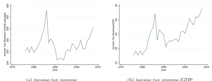
Figure 1: Evolution of the level of income tax revenue and its participation in the GDP over the period 1976-2008
400
500
600
700
Per Capita Income (R$/month)
1970 1980 1990 2000 2010
year
20
30
40
50
60
Marginal Tax Rate
1970 1980 1990 2000 2010 year
(a) Legal marginal income tax rate
0
5
10
15
n. of income tax rates
1970 1980 1990 2000 2010 year
(b) Income Tax Brackets
Figure 3: Evolution of the legal marginal income tax rate and the number of income tax brackets over the period 1976-2008
0
1
2
3
4
Average Effective Tax Rate
1970 1980 1990 2000 2010 year
(a) Average effective tax rate
2
4
6
8
Average Marginal Tax Rate
1970 1980 1990 2000 2010 year
(b) Average marginal tax rate
Figure 4: Evolution of the effective tax rate and the average marginal income tax rate over the period 1976-2008
Figure 1a shows the evolution of the income tax revenue in real terms. The data clearly shows a spike in the tax revenue in the mid-80’s, which corresponds to the period of Plano Cruzado, when Brazilian Government has frozen all the prices in the economy in an attempt to fight hyperinflation and at the same time increased significantly the real wages17. After this period, it is possible to observe an upward trend, particularly after the introduction of ‘Plano Real’ from 1995 on, which allowed the reduction of the inflation and the growth in the per capita income as shown in Figure 2. This increase might also be associated with the efficiency gains in tax collection, the expansion of formal jobs, and the increase in
17
aggregate labor supply. Figure 1b shows clearly the importance of these other reasons as there is an upward trend in the tax revenue collected as proportion of the GDP over the years (specially after the introduction of ‘Plano Real’), albeit the marginal income tax rate exhibits a downward trend, as shown in Figure 3a. Also, the average effective and marginal tax rates (Figures 4a and 4b) seem closely associated with both the tax rate of the higher income tax bracket shown in Figures 3a and the per capita income shown in Figure 2.
150
200
250
300
350
400
Income Tax Revenue (R$/month)
0 1 2 3 4
Average Effective Tax Rate
(a) Average effective tax rate
150
200
250
300
350
400
Income Tax Revenue (R$/month)
2 4 6 8
Average Marginal Tax Rate
(b) Average Marginal Tax Rate
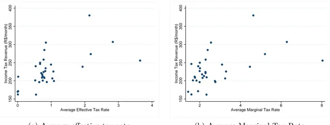
Figure 5: Scatter plot of income tax revenue against average effective and marginal income tax rate:1976-2008
The scatter plots of the raw data represented by Figures 5a and 5 shows a positive but apparently decreasing relation between the tax revenue and the effective and marginal tax rate respectively, which may be an indicative of the Laffer Curve.
Second, we use a short panel of brazilian municipalities. The panel data set we use is also based on PNAD data, aggregated at the municipal level. The sample based on a panel of municipalities is advantageous because it allows us to estimate the econometric models correcting for potential non-observed fixed effects correlated with the regressors without losing many degrees of freedom. Note that PNAD surveys individuals in 817 municipalities every non-census year. This means that we have a sample of individuals for each of the 817 municipality. 18
Another noteworthy point refers to the fact that, in general, it is not possible to identify the municipalities so we could combine different data sets. The only period for which we can identify the municipalities in PNAD, and therefore combine it with other data sets, goes from
18
1996 to 1999, making up a 4-years panel of municipalities. An advantage of such a panel is the possibility of obtaining a larger set of compatible variables given that the questionnaires assess pretty much the same variables throughout this period.
The panel sample seems adequate to estimate the labor supply response to the tax rates and other variables of interest. The required variables to estimate it such as the average number of hours worked during the week, participation rate of the working age individuals in the labor market, labor income, non-labor income, age, schooling, are all readily available from PNAD data set. As we can combine variables from different sources with this particular data set we can evaluate one of the variables of interest, the public expenditure on cash and in-kind transfers. The other control variables are also based on PNAD and are described in table 1.
Table 2 show the descriptive statistics. Since the majority of the variables both at national (country level data) and municipality levels (panel data of municipalities) come from the same source, differing only in the time span and level aggregation, it is no surprise the figures are very similar. Unfortunately, neither this survey nor other public sources of information allows one to know the amount of income tax collected at the individual or municipal level. We estimate this figure by applying the legal tax rates and deductions to the observed gross income of each individual, and then average it over the municipalities.
5
Empirical Results
5.1
Brazilian aggregated data set
according to the tests.
Table 3: Unit Root tests
Augmented Dickey-fuller
PP KPSS
H0: unit root H0: unit root H0: stationarity
Tax Revenue -2.152** -9.792 0.245
effective tax rate -2.612*** -11.568* 0.582** marginal tax rate -2.759*** -12.615* 0.598*
hours employed -1.686* -5.310 2.21***
per capita income -2.356 -12.021* 1.32***
age 4.232 1.208 3.25***
finished high school 0.596 0.322 3.25***
young 4.133 0.849 3.26***
elderly 1.593 1.209 3.22***
married 0.168 0.13 3.300***
urban -2.109 -1.675 3.19***
males -3.765*** -20.410*** 1.3***
population -2.414 -0.254 3.29***
social security -0.685 -1.936 0.698**
agriculture workers -1.557 -3.533 2.28***
n. family members -0.928 -2.767 0.914***
occupation rate -1.062 -2.332 2.21***
Debt to GDP ratio -2.256 -8.763 1.230***
total expenditures -1.703 -5.17 2.520***
Note: ∗p <10%,∗ ∗p <5%,∗ ∗ ∗p <1%. Values refer to the test statistics specifics to each test.
The estimation strategy for the tax revenue model goes as follows. We estimate our models by OLS, with Newey-West standard errors, which are robust to heteroscedasticity and autocorrelation. In the first column of table 4, we regress the income tax revenue on the average effective tax rate, its square and a constant. Then, in 5, we do likewise to assess the effects of the average marginal tax rate on tax revenue. These are called ”Short” models and under the assumption of stationarity should be able to capture long-run relation between these variabels. Next, in the second columns of each table, we include several control variables in these models, including the Debt to GDP ratio as well as the per capita public expenditure, in an attempt to account for the expenditure side on the motivation of the income tax collection. These estimations correspond to ”Full” model. Then, in the third columns of tables 4 and 5, we resort to the algorithm developed by Hendry and Krolzig (2001), Doornik (2007) and Doornik and Hendry (2007) labeled ”Auto” (short for ‘Autometrics’) to select the best specification. This approach consists of a general-to-specific (Gets) method to select the best models, i.e. the most parsimonious models with the greatest explanatory power.19 Fourth columns of tables 4 and 5 show the results of models chosen by the ‘Gets’ methodology
19
but which also include a lagged dependent variable among the candidate regressors, i.e., we test if a‘Dynamic model’ could be an appropriate choice.20 In the fifth column the non-stationary variables are made stationaries, i.e., we first-differenced them, and pick up the model through the ‘Autometrics’ algorithm. The last column brings a model chosen by the same algorithm having among the candidate regressors the ‘unit root variables’ in differences and the lagged dependent variable .21 All models from fourth column are chosen by ‘Autometrics’.22
Analyzing such models in more detail, we can see that models taxEF1 and taxM G1 suggest a concave income tax revenue function with respect to tax rates, i.e., tax rate has a positive effect on tax revenue but its squared figure has a negative impact on it. In the first model, a 1 percentage point (pp) increase on effective tax rate, increases tax revenue in R$99.996 per taxpayer, whereas for each point of increase this positive impact is diminished by R$17.787 per taxpayer.
In model taxM G1 a 1 pp increase on marginal tax rate, increases tax revenue in R$66.296 per taxpayer, while for each point of increase this positive impact is diminished by R$5.628. The AR 1-2 and ARCH 1-2 tests are presented at the bottom of the table. While we do not reject the null that the residuals exhibit not conditional heteroscedasticity (ARCH 1-2 test), we reject the null hypothesis that the residuals do not follow an autoregressive process. We test for the presence of a unit root in the residuals applying the Augmented Dick-Fuller test, and for both models we reject the presence of unit root, which indicates that the regression is not spurious.
Note that adding control variables as in modelstaxEF2 andtaxM G2 increase the explanatory power (increases the Adjusted R-square). This is probably due to the correlation these variables bear with income, which is also correlated with the effective tax rate. Model taxEF2 show a positive and significant effect of average effective tax rate on tax revenue, such that a 1 pp increase in tax rate raises tax revenue by R$98.566 per taxpayer. For each point of increase the positive effect on tax revenue is reduced by R$20.073 per taxpayer.
ModeltaxM G2 also present a positive effect such that for each pp increase in average marginal tax rate, tax revenue increases by R$59.403 per taxpayer, but the square term coefficient reveal that this effect is reduced by R$5.472 per taxpayer by additional pp increases. For both models
taxEF3 andtaxM G2 we reject the null of no autoregressive process of first and second order in the
20
In order to determine the order of the dynamic process, we analyze the autocorrelation function and the partial autocorrelation function of the income tax revenue series. The confidence interval is based on the Bartlett’s formula with 95% confidence interval. The tests indicate that a 1st order autocorrelation. These results can be obtained upon request to the authors.
21
In fact, according to West (1988), the estimates and the hypothesis testing are still valid when a right-hand variable has a unit root. Hamilton (1994, p.561), on the other right-hand, consider differencing any unit root variable before consistently estimating the model. Note that models with regressors in differences and the dependent variable in levels can be understood as the relation between short-run variables and long-run income tax revenue. The main goal with all these models is to observe whether a concavity pattern for the income tax revenues can be obtained unconditionally.
22
residuals. We also reject the null of the normality of the residuals for model taxM G2. The ADF test statistic show no evidence of unit root in the residuals of eithertaxEF2 ortaxM G2 models, indicating that the estimated models are not spurious.
Models taxEF3 and taxM G3 are defined by Hendry and Krolzig (2001) ‘Gets’ algorithm. The estimates for the first model indicates that for a 1 pp increase in the effective tax rate, tax revenue increases by R$95.198 per taxpayer. The square term is negative and statiscally significant, ans suggests the this change in tax revenue is reduced by R$19.594 for each additional percentage point increase.
Table 4: Tax revenue response to Effective and marginal tax rates taxEF1-Short taxEF2-Full taxEF3-Auto taxLagEF3-Auto URtaxEF2-Auto URtaxlagEF2-Auto
Tax Revenuet−1
effective tax rate 99.996** 98.566** 95.198*** 118.101*** 134.627*** (45.119) (45.481) (26.077) (36.924) (20.537) effective tax rate2 -17.787* -20.073* -19.594*** -24.291 -27.656***
(10.335) (10.203) (6.264) (8.992) (5.305)
males 28.074
(47.527)
hours employed # 48.254* 57.124*** 61.900*** (23.474) (16.680) (17.270)
age # 43.352 -8.027
-157.937***
45.339*
(146.098) (7.407) (51.732) (24.452) n. family members # 38.423 49.645*** 7.111 70.672*** 55.312*
(33.178) (15.035) (6.166) (16.454) (29.758)
urban # -2.648
(8.510)
finished high school # 21.018 35.821** 64.559*** (34.076) (14.463) (18.574)
social security # 12.927 17.129*** 8.921*** 38.087*** 17.752*** (10.007) (4.425) (2.359) (5.326) (5.623) formal # -7.746 -11.549*** -8.705*** -16.927*** -5.850**
(7.483) (2.556) (1.877) (3.283) (2.677) occupation rate # -16.903 -15.342** -27.163*** 22.658***
(10.230) (6.202) (6.870) (4.183)
young # -36.342 -46.163***
-175.898***
-56.612
(46.102) (14.691) (39.343) (34.399)
elderly # -193.649 -106.910* 35.569** -300.404
(255.082) (60.262) (13.581) (192.560) total expenditures # -0.000 0.008*** 0.002
(0.005) (0.002)
Debt/GDP # -0.476 -0.496 -0.682**
(0.656) (0.317) (0.312)
constant 148.669*** -346.394 1743.499*** 44.360*** (34.742) (6709.273) (564.647) (11.463)
Adjusted R2 0.251 0.558 - - 0.792
-Number of observations 32 32 32 32 32 32
AR 1-2 test (F-statistics) = 5.241 [0.012]
11.480[0.001] 8.973[0.002] 1.309 [0.293]
8.818[0.003] 2.699[0.091]
ARCH 1-2 test (F-statistics) =
0.818 [0.452]
1.251[0.302] 3.079[0.062] 1.288 [0.2917]
1.566[0.227] 0.133[0.876]
Normality test (χ2- statis-tics) =
3.610 [0.164]
4.400[0.111] 4.799[0.091] 8.407[0.015] 0.998 [0.6073]
2.702[0.259]
ADF (cointegration)
Models taxLagEF3 and taxLagM G3 (chosen by Autometrics) present the results of models with the lagged tax revenue as a regressor. They present significant coefficients for effective and marginal tax rates. In the first model, we can see that a 1 pp increase in effective tax rate leads to an increase of R$118.101 per taxpayer. As for the squared term, each additional point reduces this effect by R$24.291 per taxpayer.
On the other hand, models U RtaxLagEF2 and U RtaxLagM G2 allows for the inclusion of lagged dependent variable in the model. They are chosen by Autometrics following the ‘Gets’ procedure of Hendry and Krolzig (2001). In the first model a 1 pp increase in the effective tax rate increases tax revenue by R$134.627 per taxpayer, but such effect is reduced by R$27.656 for each additional 1 pp increase in the tax rate.
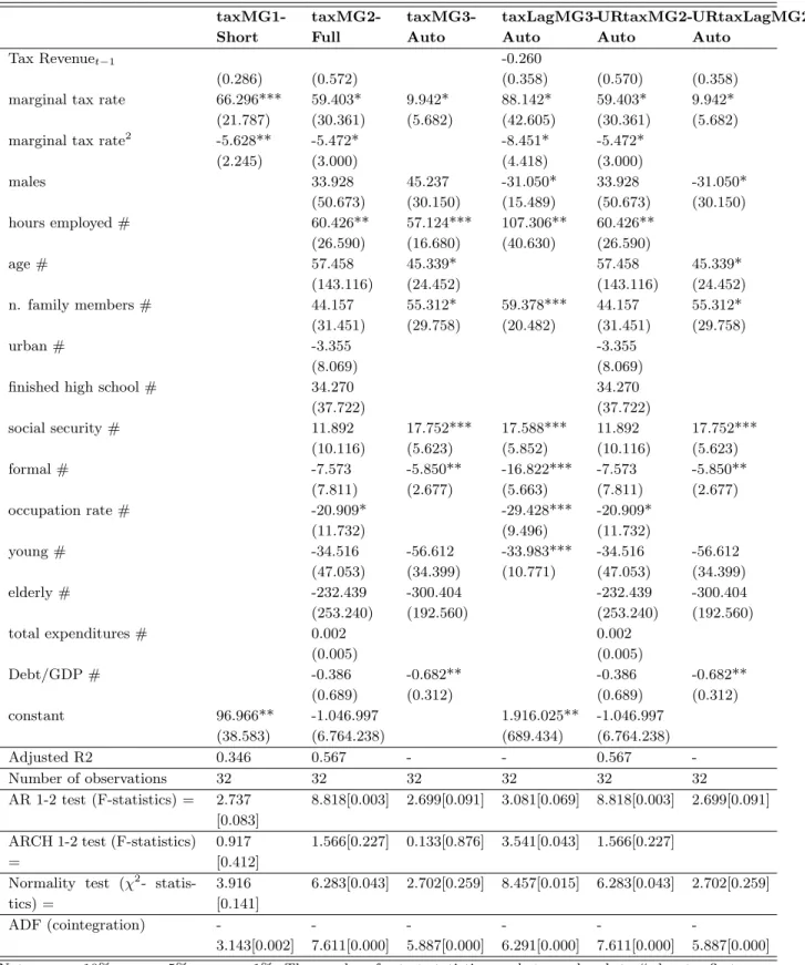
Table 5: Tax revenue response to Effective and marginal tax rates taxMG1-Short taxMG2-Full taxMG3-Auto taxLagMG3-Auto URtaxMG2-Auto URtaxLagMG2-Auto
Tax Revenuet−1 -0.260
(0.286) (0.572) (0.358) (0.570) (0.358) marginal tax rate 66.296*** 59.403* 9.942* 88.142* 59.403* 9.942*
(21.787) (30.361) (5.682) (42.605) (30.361) (5.682) marginal tax rate2 -5.628** -5.472* -8.451* -5.472*
(2.245) (3.000) (4.418) (3.000)
males 33.928 45.237 -31.050* 33.928 -31.050*
(50.673) (30.150) (15.489) (50.673) (30.150) hours employed # 60.426** 57.124*** 107.306** 60.426**
(26.590) (16.680) (40.630) (26.590)
age # 57.458 45.339* 57.458 45.339*
(143.116) (24.452) (143.116) (24.452) n. family members # 44.157 55.312* 59.378*** 44.157 55.312*
(31.451) (29.758) (20.482) (31.451) (29.758)
urban # -3.355 -3.355
(8.069) (8.069)
finished high school # 34.270 34.270
(37.722) (37.722)
social security # 11.892 17.752*** 17.588*** 11.892 17.752*** (10.116) (5.623) (5.852) (10.116) (5.623) formal # -7.573 -5.850** -16.822*** -7.573 -5.850**
(7.811) (2.677) (5.663) (7.811) (2.677) occupation rate # -20.909* -29.428*** -20.909*
(11.732) (9.496) (11.732)
young # -34.516 -56.612 -33.983*** -34.516 -56.612 (47.053) (34.399) (10.771) (47.053) (34.399)
elderly # -232.439 -300.404 -232.439 -300.404
(253.240) (192.560) (253.240) (192.560)
total expenditures # 0.002 0.002
(0.005) (0.005)
Debt/GDP # -0.386 -0.682** -0.386 -0.682**
(0.689) (0.312) (0.689) (0.312) constant 96.966** -1.046.997 1.916.025** -1.046.997
(38.583) (6.764.238) (689.434) (6.764.238)
Adjusted R2 0.346 0.567 - - 0.567
-Number of observations 32 32 32 32 32 32
AR 1-2 test (F-statistics) = 2.737 [0.083]
8.818[0.003] 2.699[0.091] 3.081[0.069] 8.818[0.003] 2.699[0.091]
ARCH 1-2 test (F-statistics) =
0.917 [0.412]
1.566[0.227] 0.133[0.876] 3.541[0.043] 1.566[0.227]
Normality test (χ2- statis-tics) =
3.916 [0.141]
6.283[0.043] 2.702[0.259] 8.457[0.015] 6.283[0.043] 2.702[0.259]
ADF (cointegration)
-3.143[0.002] -7.611[0.000] -5.887[0.000] -6.291[0.000] -7.611[0.000] -5.887[0.000]
Models U RtaxLagEF2 and U RtaxLagM G2 include all the regressors with unit root variables in differences, chosen by the Autometrics algorithm but including the lagged dependent variable. In the first model, a 1 pp increase in effective income tax rate raises tax revenue by R$134.310 per taxpayer. This effect is reduced by R$27.605 per taxpayer as the tax increase by 1 pp. The second model’s estimates indicate that tax revenue increase by R$52.409 per taxpayer in response to a 1 pp increase in marginal tax rate. The concavity revealed by the square term indicates that this effect is reduced by R$4.731 for each 1 pp increase in marginal tax rate.
The tests for all the models indicate that there is no serial correlation in the residuals. Also, there is no conditional heteroscedasticity. The residuals seem to be normally distributed and there are no unit roots in the residuals. In conclusion, models with unit root variables in differences present better properties as revealed by the tests performed on the residuals.
Looking at the models with differenced unit root variables with and without the lagged tax rev-enue (U RtaxEF2 and U RtaxM G2 versusU RtaxLagEF2 and U RtaxLagM G2) we can conclude that those present the best properties. Besides, the tax revenue function appear to have an inverse U-shape, characteristic of the Laffer Curve.
The control variables present the expected sign in the regressions with unit root variables in differences. Note that as the regressors with unit root are in differences the coefficients reflect the association between the long run tax revenue and short run variations in each of these variables. The average hours of work among employed individuals show a positive relationship with tax revenue in model U RtaxM G2.
A positive change in average age of individuals have a negative and significant impact on the income tax revenue, as suggested by models U RtaxEF2 and U RtaxLagEF2. A change in the proportion of individuals with high school degree bears a positive relation with the long run income tax revenue, as showed in models U RtaxEF2 and U RtaxLagEF2. The change in the proportion of individuals contributing to social security (which can be understood as a measure of work for-malization) and in the occupation rate show positive associations with the income tax revenue, as can be seen in modelsU RtaxEF2 and U RtaxLagM G2.
The proportion of young individuals have a negative relation with income tax revenue, as shown in modelsU RtaxEF2 andU RtaxLagM G2. The percentage of elderlies also show a negative associ-ation, but only in modelsU RtaxM G2 andU RtaxLagM G2.This is the case because those individual might be retired already and probably do receive lower income than those in the workforce.
In particular, the coefficients of two control variables present unusual signs. One case refers to the positive relation between the change in the number of family members and the tax revenue. In principle, we expect that the greater the number of children in a household, the greater is the deduction allowed in the tax base and the smaller the amount of income tax collected. However, on theoretical grounds, both signs can be justified, since larger families can also imply less time for spouses to work, and thus, less tax base to be taxed. The other case refers to the negative association verified between the percentage change in the formal workforce and the income tax revenue per taxpayer. This finding may be reflecting the fact that the ‘formality’ here is restrict to those workers of the private sector under a formal work contract. Public employees and self-employed freelance professionals are not considered formal by this variable, even though several of them earn more and pay more taxes than the ‘formal’ workers.
The variable ‘males’ - which do not present unit root according to the tests do is analyzed in levels - present mostly non-significant coefficients. But in modelU RtaxLagEF2, we find a positive and significant relation with income tax revenue. Such result is expected since the participation of males in the workforce is generally greater and the salaries of men are higher than those of women.
Finally, two of the control variables do not present statistically significant coefficients in any model. One is the proportion of urban population. The other is the Debt to GDP ratio. This last variable is expected to have a positive association with the income tax revenue, since the more indebted a country is the greater the effort to raise revenue will be to pay the services of the debt.
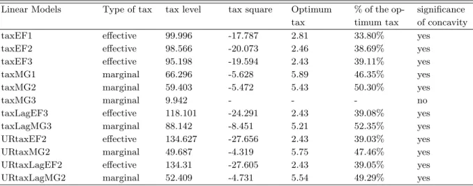
Table 6: Calculated optimum effective and marginal tax rates in Brazil - actual average effective tax=0.95, actual average marginal tax=2.73
Linear Models Type of tax tax level tax square Optimum tax
% of the op-timum tax
significance of concavity taxEF1 effective 99.996 -17.787 2.81 33.80% yes
taxEF2 effective 98.566 -20.073 2.46 38.69% yes taxEF3 effective 95.198 -19.594 2.43 39.11% yes taxMG1 marginal 66.296 -5.628 5.89 46.35% yes taxMG2 marginal 59.403 -5.472 5.43 50.30% yes
taxMG3 marginal 9.942 - - - no
taxLagEF3 effective 118.101 -24.291 2.43 39.08% yes taxLagMG3 marginal 88.142 -8.451 5.21 52.35% yes URtaxEF2 effective 134.627 -27.656 2.43 39.03% yes URtaxMG2 marginal 49.687 -4.319 5.75 47.46% yes URtaxLagEF2 effective 134.31 -27.605 2.43 39.05% yes URtaxLagMG2 marginal 52.409 -4.731 5.54 49.29% yes
5.2
Municipality level Data set - 1996-1999
Next, we move to the panel of municipalities from 1996 to 1999. This sample allows to estimate aggregated (by municipality) labor supply response to tax rate variations taking into consideration the amount of cash-cum-in-kind transfers allocated to each municipality. Moreover, such data set allows to control for the potential bias of omitted time-invariant variables once fixed effects are explicitly controlled for. Since we are trying to estimate individual decisions with aggregated data, we aggregate individual information at the municipality level using individual weights assigned by PNAD.
5.2.1 Labor supply response to average and marginal tax rates using munici-pality level data set from 1996 to 1999
Table 7 shows the fixed effects estimates of the average effective tax rate on the number of hours worked as well as on the participation rate. The results are very similar for both dependent variables and whether we use weights (size of the population) in the regression or not. Also, the estimates are analogous to those found by Foguel and Barros (2010) even though the authors use the PNAD panel from 2001 to 2005.
In this same Table, model FE-III for average hours of work shows, as expected, that a 1 per-centage point (pp) increase on the effective tax rate reduces the average number of hours worked in 1.404 hours/week. Such large response to a seemingly little variation can be explained by the fact that the average effective tax rate in Brazil for the period is as small as 0.6% of the mean income.
This same model shows that an additional R$1 on the labor income increases the labor supply in 0.005 hours/week. A 1 year variation on the mean age has a non-significant negative impact of 0.581 hours/week, though significant in models FE-IV. The proportion of elderly in the population corroborates this result, e.g. a 1 pp increase reduces in 0.189 hours/week the average labor supply. Now, an 1 pp increase in the proportion of young is associated with a 0.044 hours/week reduction (again, though not significant in this specification, it is significant in model FE-IV for average number of hours). Furthermore, a positive variation of 1pp in the proportion of non-whites has a positive impact of 0.019 hours/week.
The sector in which individuals work also has effect on labor supply. A 1 pp increase on the proportion of workers in administration, commerce and services, opposed to the proportion of workers in industry, raises the average working hours in 0.038, 0.045 and 0.073 hours/week, respectively. Possibly because industry workers in Brazil are more unionized than in other sectors, which ends up imposing constraints on the labor supply. The size of the municipality also influences the amount of working time, such that an additional 1000 inhabitants raises this figure in 0.006 hours/week. The proportion of workers paying Social Security taxes, which is used as a measure of job formality, lower the average working hours by 0.049 hours/week for a 1pp increase in the explanatory variable. On the other hand, workers engaged in agriculture activities (less formal) tend to work more since a 1 pp increase in this group raises the labor supply in 0.041 hours/week. Finally, the unemployment rate affects negatively the number of hours worked, such that a 1pp variation reduces the average working hours in 0.180 hours/week.
Finally, except for schooling that has a positive effect on labor supply according to some of the models, other control variables do not show significant results. Besides, as the estimates of the participation rate models are approximately the same as those of hours equation we are not describing those in detail here.
Table 7 also shows the estimates of the effects of the average marginal tax rate on labor supply. In this case, none of the estimates are significant. The effects of the other explanatory variables are roughly the same as those we obtain using the average effective tax rate. The only remarkable difference refers to the coefficient on non-labor income, that is negative and significant in all esti-mated models. For the hours equation, specification FE-IV indicates that a R$1 increase on the non-labor income reduces the labor supply in 0.004 hours/week, which is more consistent with the results usually found in literature on labor economics.23
23
Table 7: Labor supply (weighted population) response to Effective and Marginal Tax Rates - 1996-1999
Hours Participation Rate
effective marginal effective marginal
FE-I FE-II FE-III FE-IV FE-I FE-II FE-III FE-IV
tax rate -1.404*** -1.200*** 0.231 0.291 -4.537*** -3.958*** -0.048 0.294 (0.374) (0.391) (0.204) (0.207) (0.783) (0.821) (0.422) (0.425) labor income 0.005*** 0.005*** 0.003*** 0.003*** 0.009*** 0.009*** 0.013*** 0.012***
(0.001) (0.001) (0.001) (0.001) (0.002) (0.002) (0.002) (0.002)
age -0.581 -0.808* -0.635 -0.919* 0.099 -0.467 0.027 -0.691
(0.410) (0.440) (0.455) (0.479) (0.722) (0.791) (0.716) (0.769)
(age)2 0.008 0.012 0.009 0.014 -0.004 0.004 -0.004 0.007
0.007) (0.007) (0.008) (0.008) (0.012) (0.013) (0.012) (0.013)
schooling 0.340 0.233 0.708 0.655 0.958 0.493 1.871** 1.617
(0.463) (0.513) (0.461) (0.507) (0.877) (1.008) (0.870) (0.986)
schooling square 0.025 0.024 -0.015 -0.020 0.075 0.089 -0.019 -0.025
(0.040) (0.044) (0.040) (0.044) (0.072) (0.083) (0.074) (0.082) non-labor income -0.001 -0.000 -0.005*** -0.004** -0.001 -0.002 -0.011*** -0.012***
(0.001) (0.002) (0.001) (0.001) (0.003) (0.003) (0.003) (0.003)
young -0.044 -0.058* -0.056* -0.072** -0.064 -0.103* -0.088 -0.136**
(0.029) (0.032) (0.029) (0.032) (0.055) (0.060) (0.056) (0.061) elderly -0.189*** -0.209*** -0.164*** -0.186*** -0.515*** -0.501*** -0.456*** -0.442***
(0.050) (0.052) (0.051) (0.053) (0.090) (0.094) (0.090) (0.094)
married 0.007 0.010 0.005 0.008 0.015 0.012 0.011 0.008
(0.010) (0.010) (0.010) (0.010) (0.023) (0.023) (0.021) (0.022)
urban -0.016 -0.010 -0.016 -0.010 -0.017 0.005 -0.018 0.003
(0.019) (0.020) (0.019) (0.020) (0.042) (0.047) (0.043) (0.048)
males 0.044** 0.042* 0.050** 0.048** 0.055 0.053 0.071* 0.069
(0.022) (0.023) (0.022) (0.024) (0.042) (0.045) (0.042) (0.045) non-white 0.019*** 0.022*** 0.020*** 0.022*** 0.051*** 0.051*** 0.052*** 0.052***
(0.007) (0.007) (0.007) (0.007) (0.014) (0.015) (0.014) (0.015) workers in
adminis-tration
0.038** 0.040** 0.035** 0.035* 0.054 0.063* 0.050 0.053
(0.017) (0.018) (0.017) (0.018) 0.034) (0.036) (0.035) (0.037) workers in commerce 0.045*** 0.034** 0.046*** 0.035** 0.047 0.025 0.048 0.027
(0.015) (0.016) (0.015) (0.016) (0.032) (0.034) (0.034) (0.035) workers in services 0.073*** 0.078*** 0.079*** 0.162*** 0.169*** 0.216*** 0.177*** 0.185***
(0.018) (0.019) (0.018) (0.020) (0.033) (0.035) (0.033) (0.035)
population 0.006* 0.007** 0.003 0.004 -0.023** -0.020* 0.017* 0.018**
(0.003) (0.003) (0.003) (0.003) (0.010) (0.010) (0.009) (0.007) social security -0.049*** -0.046*** -0.047*** -0.043*** -0.180*** -0.175*** -0.174*** -0.169***
(0.011) (0.012) (0.011) (0.012) (0.022) (0.024) (0.022) (0.024) agriculture workers 0.041*** 0.042*** 0.042*** 0.220*** 0.236*** 0.217*** 0.219*** 0.237*** Continued on next page
Table 7 –Continued from previous page
Hours Participation Rate
effective marginal effective marginal
FE-I FE-II FE-III FE-IV FE-I FE-II FE-III FE-IV
(0.013) (0.013) (0.013) (0.013) (0.027) (0.029) (0.026) (0.028) n. family members -0.319 -0.258 -0.415 -0.364 -0.243 0.023 -0.571 -0.327
(0.306) (0.324) (0.304) (0.320) (0.627) (0.690) (0.616) (0.673) unemployment rate -0.180*** -0.192*** -0.187*** -0.198*** 0.213*** 0.197*** 0.189*** 0.177***
(0.014) (0.015) (0.014) (0.015) (0.030) (0.034) (0.030) (0.033)
in kind expenditures -0.404* -0.476** -1.471** -1.667***
(0.244) (0.212) (0.599) (0.503)
total expenditures 0.463* 0.409* 1.436*** 1.341***
(0.255) (0.246) (0.540) (0.514)
constant 21.777** 23.277** 28.760*** 31.117*** 24.785 31.123 43.236** 51.944*** (9.099) (9.122) (9.226) (9.340) (20.568) (20.066) (19.247) (18.826)
R2 0.361 0.379 0.351 0.373 0.323 0.324 0.296 0.303
N 3850 3652 3850 3652 3850 3652 3850 3652
F 37.215 34.465 38.259 35.639 21.055 16.027 22.573 18.026
Note: * means significant at the 10% level, ** at the 5% level and *** at the 1% level. In parentheses we report the standard errors.