Random vibration analysis design methodology applied on aircraft components - case study on a Lockheed Martin C-130H instrument panel retrofit

(1)

Ricardo Portas Marchão

Licenciado em Ciências de Engenharia Mecânica

Random vibration analysis design methodology

applied on aircraft components - case study on a

Lockheed Martin C-130H instrument panel retrofit

Dissertação para obtenção do Grau de Mestre em

Engenharia Mecânica

Orientador: Prof. Doutor João Cardoso, Professor

Auxiliar, FCT-UNL

Co-orientador: Eng. João Rui Duarte, Engenheiro

de Projeto, OGMA S.A

Júri:

Presidente: Tiago Alexandre Narciso da Silva, Professor Auxiliar Convidado, FCT/UNL

Vogais: Carlos Manuel de Andrade Rodrigues, Engenheiro de Projecto, OGMA

João Mário Burguete Botelho Cardoso, Professor Auxiliar, FCT/UNL

(2)

(3)

Random vibration analysis design methodology applied on

aircraft components - case study on a Lockheed Martin C-130H

instrument panel retrofit

Copyright @ Ricardo Portas Marchão, Faculdade de Ciências e Tecnologia, Universidade Nova

de Lisboa

A Faculdade de Ciências e Tecnologia e a Universidade Nova de Lisboa têm o direito, perpétuo

e sem limites geográficos, de arquivar e publicar esta dissertação através de exemplares impressos

reproduzidos em papel ou de forma digital, ou por qualquer outro meio conhecido ou que venha

a ser inventado, e de a divulgar através de repositórios científicos e de admitir a sua cópia e

distribuição com objetivos educacionais ou de investigação, não comerciais, desde que seja dado

(4)

(5)

Ricardo Portas Marchão

Licenciado em Ciências de Engenharia Mecânica

Random vibration analysis design methodology applied on

aircraft components - case study on a Lockheed Martin C-130H

instrument panel retrofit

Dissertação apresentada à Faculdade de Ciências e Tecnologia da Universidade Nova de Lisboa

para a obtenção do grau de Mestre em Engenharia Mecânica

(6)

(7)

(8)

(9)

i

Acknowledgements

I would like to express my gratitude to all of whom were involved throughout the development

of this dissertation because it would not have been possible without them. My effort and

commitment would not have been enough to achieve my dissertation objectives without their

contribution:

To Dr. João Cardoso for his guidance and support throughout the whole process, and for making

this project possible.

To Eng. João Rui Duarte for his support, commitment and availability during the whole process

which was essential to carrying out this dissertation.

To OGMA-Indústria Aeronáutica de Portugal, S.A. and its collaborators which integrated me in

their workplace and helped me when it was necessary.

To all Professors that I was able to learn from and contributed to the success of my academic

career. I am very grateful to them for transmitting me knowledge and for clarifying my doubts

and questions whenever I needed.

Finally, I would like to thank my parents for the unconditional support and for being always on

(10)

(11)

iii

Abstract

In the aeronautical industry, qualification and certification processes are very complex not only

because safety has to be ensured, but also because there is regulation that must be fulfilled.

This dissertation has its origin on the necessity of assisting a design certified company credited

as DOA (Design Organization Approval) in a preliminary phase of a modification project, and

fulfill the need of developing an analysis methodology at a preliminary design phase that allows

to produce confident results in a short time.

The modification in study consists in a flight instruments retrofit (upgrade) for Lockheed Martin

C-130 H aircraft series. One of the main concerns on the modified instrument panel is its level of

vibration.

Random vibration is recognized as the most realistic method of simulating the dynamic

environment of military applications. PSD (Power Spectral Density) is a statistical measure

defined as the limiting mean-square value of a random variable and it is used in random vibration

analyses in which the instantaneous magnitudes of the response can be specified only by

probability distribution functions that show the probability of the magnitude taking a certain

value.

The purpose of this work is a creation of an efficient methodology which is intended to provide

guidance for future possible projects of modification and fulfills the requirements of

MIL-STD-810G.

The design methodology was implemented in a case study: the Lockheed Martin C-130H

instrument panel retrofit (upgrade). Case study simulations were carried out through FEM (Finite

Element Method).

Keywords: Power Spectral Density (PSD), Random Vibration, Design Methodology, Finite

(12)

(13)

v

Resumo

Na indústria aeronáutica, os processos de qualificação e certificação podem ser muito complexos

não só porque a segurança tem de ser assegurada, mas também porque há regulamentação que

tem de ser cumprida.

Esta dissertação surge com o intuito de apoiar uma empresa certificada para realizar projetos

creditada como DOA (Design Organization Approval), numa fase preliminar do projeto de

modificação, cumprindo a necessidade desenvolvendo uma metodologia de análise na fase

preliminar de projeto que permita produzir resultados fidedignos num curto período de tempo.

A modificação em estudo consiste na modernização dos instrumentos de voo para a gama de

aeronaves Lockheed Martin C-130 H. Uma das principais preocupações em relação ao novo

painel de instrumentos é o seu nível de vibração.

O método mais consistente de simular o ambiente dinâmico de aplicações militares é através de

vibrações aleatórias. O PSD (Power Spectral Density) é uma medida estatística que se define

limitando o valor médio quadrático de uma variável aleatória e é usado em análises de vibrações

aleatórias em que as magnitudes instantâneas da resposta são especificadas por funções de

distribuição de probabilidade que mostram a probabilidade dessa resposta atingir um determinado

valor.

O objetivo deste trabalho é a criação de uma metodologia eficiente que se destina a fornecer

orientação para futuros possíveis projetos de modificação que cumpram os requisitos da norma

MIL-STD-810G.

A metodologia de projeto foi implementada num estudo de caso: o painel de instrumentos da

aeronave Lockheed Martin C-130H. As simulações do estudo de caso foram realizadas através de

uma análise de elementos finitos.

Palavras-Chave: Densidade Espectral, Vibrações Aleatórias, Metodologia de Projeto, Análise

(14)

(15)

vii

List of Contents

1 Introduction ... 1

1.1 Motivation ... 1

1.2 Objectives ... 3

1.3 Thesis Structure ... 4

2 Confidence Assurance in Engineering Simulation ... 5

2.1 Quality Management in Engineering Simulation ... 5

2.2 Verification and Validation Processes ... 6

3 Theoretical Framework ... 9

3.1 Non-random Vibration Analysis Background ... 9

3.1.1 Harmonic Motion ... 9

3.1.2 Undamped free vibration ... 10

3.1.3 Damped Free Vibration ... 12

3.1.4 Forced Vibration ... 14

3.2 Random Vibration Analysis Background... 19

3.2.1 Types of signal ... 19

3.2.2 Random vibration ... 21

3.2.3 Gaussian distribution ... 24

3.2.4 Statistical Properties of Random Vibration ... 26

3.2.5 How to calculate PSD ... 28

3.2.6 The meaning of gRMS in sine and random vibration ... 31

3.2.7 Dynamic analysis ... 32

4 Aeronautic Regulation ... 35

4.1 Scope of change ... 35

4.2 Regulations ... 36

(16)

viii

5 Case Study ... 43

5.1 Introduction ... 43

5.2 Finite Element Method ... 43

5.3 Material Properties ... 44

5.4 Strategic simplifications ... 45

5.5 Elements ... 46

5.6 Connections ... 48

5.7 Mesh ... 49

5.8 Boundary Conditions... 51

5.9 Natural Frequencies... 51

5.10 Geometries ... 54

5.10.1 Structure I ... 54

5.10.2 Structure II... 55

5.10.3 Structure III ... 56

6 Results ... 59

6.1 Structure I ... 59

6.1.1 X-axis input simulation ... 60

6.1.2 Y-axis input simulation ... 62

6.1.3 Z-axis input simulation ... 64

6.1.4 Data Evaluation ... 65

6.2 Structure II ... 67

6.2.4 Data evaluation ... 73

(17)

ix

6.3.4 Data evaluation ... 81

6.4 Concluding Remarks ... 82

7 Vibration Isolation... 85

8 Methodology ... 91

9 Conclusions ... 95

9.1 Concluding remarks ... 95

9.2 Future considerations ... 96

10 Bibliography ... 99

11 Appendix A ... 103

11.1 The Fourier Transform ... 103

11.1.1 Discrete Fourier Transform ... 106

11.1.2 Fast Fourier Transform ... 107

(18)

(19)

xi

List of Figures

Figure 1.1 - Information versus cost changes during product development (adapted from [3]) ... 2

Figure 1.2-The Iron Triangle[8] ... 2

Figure 1.3 - Thesis work flowchart ... 3

Figure 2.1 - ISO 9001:2008 Quality Management System model [10] ... 5

Figure 2.2 - Three pillars of engineering design on the foundations of Verification and Validation ... 6

Figure 2.3 - Simulation and V&V process flow diagram [12] ... 7

Figure 2.4 - Application of the simulation process [12] ... 7

Figure 3.1 - Harmonic Motion ... 9

Figure 3.2 - Undamped single-degree-of-freedom system ... 11

Figure 3.3 – Mass-spring system [14] ... 12

Figure 3.4- System responses[15] ... 14

Figure 3.5 - Excited system with harmonic force ... 14

Figure 3.6 - Total Response of the System[16] ... 15

Figure 3.7 - Gain function for force-excited system[17] ... 16

Figure 3.8 - Base-excited system ... 17

Figure 3.9 - Gain function for base-excited system (absolute displacement)[17] ... 18

Figure 3.10 - Gain function for base-excited system (relative displacement)[17] ... 19

Figure 3.11 - Mono-frequent time signal ... 20

Figure 3.12 - Multi-frequent time signal ... 20

Figure 3.13 - Pseudo-stochastic[19] ... 20

Figure 3.14 - Pulse type time signal ... 20

Figure 3.15 - Step type time signal ... 20

Figure 3.16 - Sine sweep time signal[20] ... 20

Figure 3.17 - White noise (frequency domain) ... 21

(20)

xii

Figure 3.19 -Narrow-band (frequency domain) ... 21

Figure 3.20 - Deterministic and Random Excitation [22] ... 22

Figure 3.21- Random and Sine Waves[24] ... 23

Figure 3.22- White Light Passed Through a Prism ... 23

Figure 3.23 - Random vibration signal analogy with white light ... 24

Figure 3.24 - Gaussian distribution [27] ... 25

Figure 3.25 - Transformation of a time signal in a histogram ... 27

Figure 3.26 - Equivalence between grmsand σ ... 27

Figure 3.27 - Statistical Properties of a Random Vibration Signal ... 28

Figure 3.28 - Spectral analysis procedure using analog filters ... 29

Figure 3.29 - Calculation of a Power Spectral Density in a standardized unit of measure ... 30

Figure 3.30 - PSD calculation technique ... 31

Figure 3.31 – grms on a sine test ... 32

Figure 3.32 – grms on random test ... 32

Figure 3.33 - Dynamic Analysis Methodology ... 32

Figure 3.34 - Eigenvalues solution ... 33

Figure 3.35 - Transfer Function 𝐻𝑓. ... 33

Figure 3.36 - PSD input and PSD response ... 34

Figure 4.1- Lockheed Martin C-130H ... 35

Figure 4.2 - Analog Instrument Panel ... 35

Figure 4.3 - Digital Instrument Panel ... 35

Figure 4.4 - Vibration environment categories ... 37

Figure 4.5- Preparation for test - preliminary steps... 37

Figure 4.6 - Propeller aircraft vibration exposure (1)[31] ... 39

Figure 4.7 - Propeller aircraft vibration exposure (2)[31] ... 39

Figure 4.8 - Propeller vibration exposure that will be applied as input in all simulation analysis ... 40

(21)

xiii

Figure 5.2 - Simulation Methodology ... 44

Figure 5.3 – Chamfers and notches simplification ... 45

Figure 5.4 - Geometry simplification ... 45

Figure 5.5 - Bolts simplification ... 46

Figure 5.6- Solid187 in comparison to a 4-node tetrahedral element ... 46

Figure 5.7 - Solid186 in comparison to an 8-node cube element ... 47

Figure 5.8 - Target170-Conta174 and Targe170-Conta175 Contact Pairs ... 47

Figure 5.9 - Beam188 Element ... 47

Figure 5.10 - Shell181 Element ... 48

Figure 5.11 - Bolt-sheet plate, beam-sheet plate, body-ground interactions ... 48

Figure 5.13 - Part meshed with solid elements ... 50

Figure 5.12 - Part meshed with shell elements ... 50

Figure 5.14 - Boundary Conditions ... 51

Figure 5.15 - Boundary Conditions Localization ... 51

Figure 5.16 - Fixation on areas A, B, C, D... 52

Figure 5.17 - Fixation on areas E, F, G, H ... 52

Figure 5.18 - Fixation on areas A, B, C, D for simulation 6 ... 52

Figure 5.19 - Structure I ... 54

Figure 5.20 - Structure II ... 55

Figure 5.21 - Structure III ... 56

Figure 6.1 - Color scale ... 59

Figure 6.2 - Coordinate system ... 59

Figure 6.3 - Identification of points that will provide information about PSD response (1)... 61

Figure 6.4 - PSD response of point 1 and clarification of the concepts peak value and most critical frequency ... 61

(22)

xiv

Figure 6.13 - Identification of most critical areas ... 83

Figure 6.14 - Glare-shield ... 83

Figure 6.15 - Center panel engine indicator ... 83

Figure 7.1 - Localization of damping isolators ... 85

Figure 7.2 - Isolator using friction damped spring ... 86

Figure 7.3 - Amplification and isolation regions ... 87

Figure 7.4 - L44 Dimensional Drawing ... 88

Figure 8.1 - Transformation of inputs and outputs ... 91

Figure 8.2 – FEM Modelling sub-process ... 92

Figure 8.3 - Shock mounts installation sub-process ... 92

Figure 8.4 - Random vibration sub-process ... 93

Figure 9.1 - Equivalent sinusoidal history... 97

Figure 11.1-Relationship between time domain and frequency domain[46] ... 103

Figure 11.2- Arbitrary periodic function of time[47] ... 103

Figure 11.3 - Real and imaginary Fourier coefficients ... 105

Figure 11.4 - The Fourier density spectrum ... 105

Figure 11.5 - Analog to Digital Conversion [50] ... 106

Figure 11.6 - Buffer example ... 108

Figure 11.7 - Discontinuity between repeating buffers results in spectral leakage ... 108

Figure 11.8 - Hanning window function ... 108

Figure 11.9 - Reduction of spectral leakage by multiplying the signal with a window functio 109

Figure 11.10 - 50% Overlapping ... 109

(23)

xv

List of Tables

Table 3.1 - Types of stationary signals ... 20

Table 3.2- Differences between sinusoidal and random vibration ... 22

Table 3.3 - Probability of random amplitudes (1) ... 25

Table 3.4 - Probability of random amplitudes (2) ... 25

Table 3.5 - Influence of the bandwidth filter on measurements ... 29

Table 4.1 - ASD level of vibration calculation ... 40

Table 5.1 - Mechanical Properties of Aluminum 2024-T3 ... 44

Table 5.2 - Mesh characteristics on Workbench 17.0 ... 49

Table 5.3- Comparison of generated elements according to solid and shell formulation ... 50

Table 5.4 - Comparison of number of elements between a 3D mesh without simplifications and

2D mesh with simplifications ... 50

Table 5.5 - Fixation types applied for all simulations ... 52

Table 5.6 – Natural Frequencies Results ... 53

Table 5.7 - Structure I element types ... 54

Table 5.8 - Structure I model properties ... 55

Table 5.9 - Structure II element types ... 55

Table 5.10 - Structure II model properties ... 56

Table 5.11 - Structure III element types ... 56

Table 5.12 - Structure III model properties ... 57

Table 5.13 - Representation of instruments as lumped point masses ... 57

Table 6.1 - Structure I Natural Frequencies ... 59

Table 6.2 - Structure I most critical areas after X-Axis Input ... 60

Table 6.3 - Most critical results after X-Axis Input ... 60

Table 6.4 - Range of excitation frequencies generated by the propeller ... 61

Table 6.5 - PSD response for X-axis excitation ... 62

(24)

xvi

Table 6.7 - Most critical results after Y-Axis Input ... 63

Table 6.8 - PSD response for Y-axis excitation ... 63

Table 6.9 - Structure I most critical areas after Z-Axis Input ... 64

Table 6.10 - Most critical results after Z-Axis Input ... 64

Table 6.11 - PSD response for Z-axis excitation ... 65

Table 6.12 - Structure I data collection ... 66

Table 6.13 - Number of points whose critical frequency is within the range of propellers ... 66

Table 6.14 – Structure II Natural Frequencies ... 67

Table 6.15 -Structure II most critical areas after X-Axis Input ... 67

Table 6.18 – Structure II most critical areas after Y-Axis Input ... 69

Table 6.21 – Structure II most critical areas after Z-Axis Input ... 71

Table 6.22 - Most critical results after Z-Axis Input ... 72

Table 6.24 - Structure II data collection ... 73

Table 6.26 - Structure III Natural Frequencies... 74

Table 6.27 - Structure III most critical areas after X-Axis Input ... 75

Table 6.30 - Structure III most critical areas after Y-Axis Input ... 77

Table 6.33 - Structure III most critical areas after Z-Axis Input ... 79

(25)

xvii

Table 6.36 - Structure III data collection ... 81

Table 6.38 - Overall data collection ... 82

Table 7.1 - L-Mount Specifications ... 85

Table 7.2 - L44 Height of aluminum core ... 89

Table 8.1 - Meaning of flowchart symbols ... 91

(26)

(27)

xix

Acronyms and Nomenclature

AFM – Aircraft Flight Manual

ANAC – Autoridade Nacional da Aviação Civil

ASD – Acceleration Spectral Density

c – Damping Coefficient

𝑐𝑐– Critical Damping Coefficient

CPM – Cycles per Minute

DFT – Discrete Fourier Transform

DOA – Design Organization Approval

EASA – European Aviation Safety Agency

𝑓– Frequency 𝐹𝑜 – External Force

Fc – Center Frequency

Fd – Disturbing Frequency

FEA – Finite Element Analysis

FEM – Finite Element Method

FFT – Fast Fourier Transform

𝐹𝑛– Natural Frequency

𝐹𝑛,𝑚𝑖𝑛– Minimum Isolator Natural

Frequency

𝑔𝑟𝑚𝑠 – Root Mean Square Acceleration

Hf – Transfer Function

ICAO – International Civil Aviation

Organization

ISO – International Organization for Standardization

k – Spring Constant

m – Mass

MS – Margin of Safety

OEM – Original Equipment Manufacturer

PSD – Power Spectral Density

𝑃𝑆𝐷𝑖𝑛– Input Power Spectral Density

𝑃𝑆𝐷𝑜𝑢𝑡– Output Power Spectral

Density

QMS – Quality Management System

𝑟– Frequency Ratio

RMS – Root Mean Square

RPM – Revolutions per Minute

T – Transmissibility

𝑇𝑟– Resonant Transmissibility

V – Level of Isolation

V&V – Verification and Validation

𝜔𝑛– Natural Frequency

𝑋̅– Mean

𝑋2

̅̅̅̅_– Mean Square

𝛿𝑒𝑠𝑡– Static Equilibrium Position

𝜉– Damping Factor σ – Standard Deviation

𝜏– Period

(28)

(29)

1

1 Introduction

1.1 Motivation

In the aeronautical industry, modification and design processes always carry an associated risk.

These processes are very complex not only because safety has to be ensured, but also because

there is regulation that must be fulfilled [1].

The design process is a very important stage in the development of a product. The committed

costs with this stage are about 80% of the overall cost of a project, the majority of decisions are

made by the end of this stage. On the other hand, the committed costs with manufacturing are

only about 5% [2]. This concept clarifies the importance of making a decision in the design phase.

Figure 1.1 represents the variation of the cost when modifications are implemented, information

about the product and the possibility to modification process over time [3]. This fact justifies the

need to carefully proceed with the modification project, from the early stages of the design process

in order to obtain the most efficient design with lesser costs and better quality in a perfect balance

with time.

The focus of this work is to create a methodology for modification of aircraft design which meets

all the standard requirements in the aeronautical industry. This dissertation has its origin on the

necessity of assisting a design certified company credited as DOA (Design Organizational

Approval) in a preliminary phase of project modification.

An organization credited as DOA has some privileges as to classify modifications and repairs as

major or minor, approve modifications and minor repairs, approve major repairs and approve

minor revisions to the AFM (Aircraft Flight manual), among others.

Currently, aeronautical standards and certifications are managed by international organizations

[4]. ICAO (International Civil Aviation Organization) is a specialized United Nations agency that

regulates international civil aviation since the Chicago Convention on the International Civil

Aviation, held in Chicago in 1944 [5]. EASA (European Aviation Safety Agency) is the

organization which assists member states of the European Union to meet its obligations to the

ICAO. EASA aims to promote the highest standards of safety and environmental protection in

civil aviation of the European Union. This organism has the right to approve organizations

involved in the design, production and maintenance of aircraft components [6]. In Portugal, the

(30)

2

Another motivation for this dissertation is the case study that was chosen to validate the

methodology: the instrument panel modification of a Lockheed Martin C-130 H. This case

allowed me to learn about the processes of certification and qualification in aeronautical industry.

A dynamic study on the modified structural components is very important in order to prevent that

their natural frequencies and vibration modes approach the excitation frequencies. Without this

study, it may run up risks of undesired vibrations that can cause, for example, wear by fatigue in

aircraft components. Another risk which is vital to be avoided is the vibration of the instrument

panel, which in turn can disturb its readability by the pilot.

The present work can be very useful and its purpose is to serve as a reference when the company

will be starting the future modification projects.

Figure 1.1 - Information versus cost changes during product development (adapted from [3]) The success of a project management depends on the perfect balance between Quality, Time and

Cost. These are the main concerns when developing a methodology for a project design. The

methodology carried out in this dissertation aims to increase the quality of the design phase of the

modification project while reducing cost and time. On Figure 1.2, it is represented the model of

the Iron Triangle presented by Roger Atkinson[8].

Figure 1.2-The Iron Triangle[8]

The development of this dissertation resulted in a cooperation between Faculdade Ciências e

(31)

3

1.2 Objectives

This dissertation aims to develop a methodology for aircraft components modification. It is

intended to develop a useful tool for a project team which allows a DOA to obtain, efficiently, a

final solution that complies with existing certification requirements in the aviation industry.

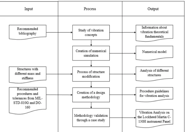
The study was carried out through the flowchart described on Figure 1.3 - Thesis work flowchart. The outputs described in the flowchart represent the thesis milestones in order to achieve the

major objective of this dissertation, which was the implementation of recommended procedure

guidelines for a vibration analysis on a modified structure.

The methodology was applied through a case study: the instrument panel vibration analysis after

a flight instruments retrofit (upgrade) for Lockheed Martin C-130 H aircraft series.

(32)

4

1.3 Thesis Structure

The inherent information provided by this dissertation is distributed along nine chapters regarding

its main purpose which is the vibration analysis methodology on modified aircraft components.

 The first chapter refers to the motivation and a brief description of the entities that

regulate the international aeronautical standards. The thesis main objectives and

milestones are also included and they are expressed in the flowchart of the dissertation

outputs.

 The second chapter is an introductory approach to quality management system in

engineering simulation and the processes of verification and validation in engineering

design.

 The third chapter is a comprehensive explanation of vibration analysis fundamentals. On

this chapter, it is reviewed the concepts of one degree of freedom including the notion of

resonance. The concept of Power Spectral Density (PSD) and its importance of measuring

vibration is clarified. This chapter also includes an overview of several types of signals.

It also clarifies the difference between harmonic and random vibration analyses.

 The fourth chapter is related to certification process according with international

standards. The procedures and tolerances which were taken into consideration on the

simulations are presented in this chapter.

 The fifth chapter presents the case study as well as considerations about the Finite

Element Method. Modeling decisions about material properties, implemented

simplifications, meshing and connections are referred. Details about structure geometries

which will be simulated in a Finite Element Analysis are discussed.

 The sixth chapter shows the obtained PSD results after performing the recommended

vibration simulations. A detailed discussion of the results is also included.

 On the seventh chapter, the methodology of a shock mount selection is addressed. The

theory related to vibration isolation is clarified by choosing the most appropriate mount,

the verification procedure is also presented. This chapter is related to the shock mount

selection procedure according to the suggested methodology by the OEM (Original

Equipment Manufacturer)

 The eighth chapter aims to clarify the definition of the procedures to be followed during

the proposed modification methodology.

 The ninth chapter includes final remarks and conclusions of this dissertation and also

(33)

5

2 Confidence Assurance in Engineering Simulation

2.1 Quality Management in Engineering Simulation

The ISO 9000 family of standards provides guidance and tools for companies and organizations

that want to ensure that their product and services consistently meet customers´ requirements and

that quality is continually improved. There are three standards: ISO 9000 covers the basic

concepts of quality management and associated language, ISO 9001 sets out the requirements of

a Quality Management System (QMS). The ISO 9002 and ISO 9003 standards were incorporated

into ISO 9001 standard. ISO 9004 focuses on how to make a QMS more efficient [9].

The primary purpose of the QMS is to provide the framework for an organization´s management

process. Instituting a quality management system will ensure that quality principles are built into

the simulation production process at a fundamental level, thereby facilitating quality control in

all aspects of the work. The quality system will provide a framework within which simulation

work can be properly planned and executed under controlled conditions to achieve consistent

simulation product quality. The usual purpose of an engineering simulation is to predict the

behavior of an engineered object or system in order to assess its ability to support design loadings.

The success of the simulation will be strongly influenced by the quality of its planning, process,

verification and validation activities. On Figure 2.1, it is presented the QMS model for

engineering simulation.

Figure 2.1 - ISO 9001:2008 Quality Management System model [10]

The QMS requires a tool to access the design process, of which the simulation process is a core

component; this tool is largely the process of Verification & Validation (V&V) which is a

(34)

6

2.2 Verification and Validation Processes

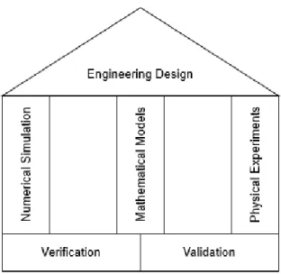
A sound engineering design is supported on the three pillars of numerical simulation,

mathematical models and physical experiments as presented on Figure 2.2. The goal of good

simulation governance is to match numerical simulation with physical experiments. This cannot

be done in any rational manner without consideration of the mathematical models that govern the

physics of the problem. Whilst the two terms, at first sight, may appear to be almost synonyms,

the processes of verification and validation are different. They provide the foundations for

engineering design by tying together the three pillars of engineering design, these cannot exist

without the mathematical models [11].

Figure 2.2 - Three pillars of engineering design on the foundations of Verification and Validation

The process of verification and validation is the mechanism used to demonstrate that a simulation

is robust and that it has been performed using best practices. The major concern in engineering

simulation is the degree to which a simulation model can accurately represent the real word

behavior. Any model of an engineered system will necessarily be approximate and simulation

error will inevitably be introduced. Therefore, before any real confidence can be placed in

predictions of the model, it needs to be demonstrated that the model is capable of accurately

predicte the real world engineering behavior and generate results that are valid for the purpose of

engineering design substantiation. This can be achieved through the application of appropriate

(35)

7

The simulation process is presented on Figure 2.3 and an application of this process is presented

on Figure 2.4.

Figure 2.3 - Simulation and V&V process flow diagram [12]

Figure 2.4 - Application of the simulation process [12]

Verification is the process of determining that a computational model accurately represents the

underlying mathematical model and its solution. Validation is the process of determining the

degree to which a model is an accurate representation of the real world. Both processes are related

to one another and are taken into account in the Quality Management System model applied for

engineering simulation.

Good simulation governance, which enables the practicing engineer to have confidence in his

results, is all about matching the results from numerical simulation with whenever possible, those

of physical experiments, and must take place regarding mathematical models. Verification is the

process which ensures the quality of the match between the numerical simulation results and the

mathematical model. Simulation process has been updated based on supporting physical

experiments along years providing more confidence assurance in engineering simulation.

Finite Element Analysis (FEA) has become widely used and globally accepted in many industry

sectors. FEA is a powerful technique which can produce solutions to challenging structural

analysis problems. The technology and computational efficiency of the method, together with the

rapid increases in computer processing power means that nowadays the scope and size of

(36)

(37)

9

3 Theoretical Framework

This chapter contains a description of vibration analysis fundamentals. On this chapter, it will be

reviewed the concepts of one degree of freedom including the notion of resonance. The concept

of Power Spectral Density (PSD) and its importance for measuring vibration is clarified. This

chapter also includes an overview of several types of signals. Differences between sine and

random vibration analysis are explained.

3.1 Non-random Vibration Analysis Background

3.1.1 Harmonic Motion

It is important to understand the fundamentals of vibration theory. On the following paragraphs,

the concepts and definitions associated with linear and elastic vibrations of systems with a single

degree of freedom will be reviewed. These systems only require one coordinate to describe their

position at any instant of time.

On Figure 3.1 it is shown a vector OP with a length 𝐴 that rotates counterclockwise with constant angular velocity 𝜔. The angle that OP makes with the horizontal axis at any time 𝑡 is represented by 𝜃 = 𝜔𝑡. The projection of OP on the vertical axis is represented by 𝑥 in (3.1):

𝑥 = 𝐴 sin 𝜔𝑡 (3.1)

As seen before, 𝑥 is a function of time. This function which is represented on Figure 3.1 is called the harmonic motion.

(38)

10

These are some basic definitions of harmonic motion [13]:

 A represents the amplitude. The range of 2𝐴 represents the peak-to-peak displacement.

 The period is the time for the motion to repeat and it is represented by 𝜏 in (3.2):

ω𝜏 = 2𝜋 (3.2)

 A cycle is the motion in one period.

 Frequency is the number of cycles per time unit, usually it is expressed in Hz. In terms of

the period, the frequency is represented as (3.3):

𝑓 =1_𝜏 (3.3)

From (3.3) the frequency is related to ω as (3.4):

𝑓 =_2𝜋𝜔 (3.4)

 The velocity of a particle is (3.5):

𝜈 =𝑑𝑥

𝑑𝑡 = 𝑥̇ (3.5)

 The acceleration of a particle is (3.6):

𝑎 =𝑑𝜈 𝑑𝑡 =

𝑑2_𝑥

𝑑𝑡2 = 𝑥̈ (3.6)

Thus, in harmonic motion displacement, velocity and acceleration are related by (3.7), (3.8) and

(3.9):

𝑥 = 𝐴 sin 𝜔𝑡 (3.7)

𝜈 = 𝑥̇ = 𝐴𝜔 cos 𝜔𝑡 (3.8)

𝑎 = 𝑥̈ = −𝐴𝜔2_{sin 𝜔𝑡}

(3.9)

3.1.2 Undamped free vibration

Figure 3.2 shows a spring-mass system with a single degree of freedom. The spring is originally

in the unstretched position. It is assumed that the spring obeys Hook´s law. In (3.10), 𝐹 represents the force in the spring and 𝑘 represents the spring constant.

(39)

11

When the mass 𝑚 is added in, the spring deflects to a static equilibrium position represented as 𝛿𝑒𝑠𝑡. If the mass is perturbed and allowed to move dynamically, the displacement measured from

the equilibrium position represented as 𝑥 is a function of time. 𝑥 (𝑡) represents the absolute motion of the mass. The equations of motion are employed to determine the position as a function of

time. The free-body diagrams are shown on Figure 3.2. Applying Newton’s second Law, it is

obtained (3.11)

𝑊 − 𝑘(𝑥 + 𝛿𝑒𝑠𝑡) = 𝑚𝑥̈ (3.11)

Figure 3.2 - Undamped single-degree-of-freedom system

As seen from the static condition, 𝑊 = 𝑘𝛿_𝑒𝑠𝑡. Therefore the equation of motion results in (3.12):

𝑚𝑥̈ + 𝑘𝑥 = 0 (3.12)

Equation (3.12) is considered as a linear differential equation of second order with the solution of

the type:

𝑥(𝑡) = 𝐶𝑒𝑠𝑡 _(3.13)

Performing the Laplace Transform:

𝜁{𝑚[𝑥̈(𝑡)]} + 𝜁{𝑘[𝑥(𝑡)]} = 𝜁{0} (3.14)

⇔ 𝑠2_{𝑚 + 𝑘 = 0} _(3.15)

(40)

12

⇒ 𝑠 = ±𝑖√_𝑚𝑘 (3.16)

The natural frequency of the system is shown in (3.17):

𝑤𝑛 = √_𝑚𝑘 (3.17)

Replacing s on the equation 𝑥(𝑡) = 𝐶𝑒𝑠𝑡 , the response of the system results in (3.19):

𝑥(𝑡) = 𝐶1𝑒𝑖𝑤𝑛𝑡+ 𝐶2𝑒−𝑖𝑤𝑛𝑡 (3.18)

⇔ 𝑥(𝑡) = 𝐴1cos(𝑤𝑛𝑡) + 𝐴2sin(𝑤𝑛𝑡) (3.19)

The constants 𝐴₁ and 𝐴₂ are calculated from the initial conditions:

For x(t), t=0 ⇒𝐴₁= 𝑥₀ For 𝑥̇(𝑡), t=0 ⇒𝐴₂= 𝑥0̇

𝑤𝑛

(3.20)

3.1.3 Damped Free Vibration

On Figure 3.3 it is shown the spring-mass system with an energy-dissipating mechanism

described by the damping force. This force is proportional to the velocity of the mass. The

damping coefficient is represented by 𝑐. Applying Newton’s second law, this model leads to the following linear differential equation of second order (3.21):

𝑚𝑥̈ + 𝑐𝑥̇ + 𝑘𝑥 = 0 (3.21)

Assuming the solution 𝑥(𝑡) = 𝐶𝑒𝑠𝑡, the characteristic equation is represented in (3.22):

𝑠2_{𝑚 + 𝑐𝑠 + 𝑘 = 0} _(3.22)

Its roots are represented in (3.23):

𝑠1,2=_{2𝑚 ±}−𝑐 √(_2𝑚)𝑐 2

−_𝑚𝑘 (3.23)

Figure 3.3 – Mass-spring system [14]

W 𝑐𝑥̇

(41)

13

The critical damping coefficient 𝑐_𝑐 is defined when that value c makes the radical equal to zero and it is represented in (3.24):

⇒ 𝑐𝑐 = 2𝑚𝑤𝑛 (3.24)

The damping factor is defined in (3.25):

ξ =_𝑐𝑐

𝑐 (3.25)

There are three different cases which generates three different responses of the system: over

damping, critical damping and under damping.

Over damping occurs when 𝑐 > 𝑐_𝑐. Both roots are real and the solution to the differential equation (3.21) is represented in (3.26).

𝑥(𝑡) = 𝐴𝑒𝑠1𝑡_{+ 𝐵𝑒}𝑠2𝑡 _(3.26)

The constants of integration are represented as 𝐴 and 𝐵. 𝑠₁ and 𝑠₂ will be both negative. Therefore, given an initial displacement, the mass will decay to its equilibrium position without oscillating

motion.

Critical Damping occurs when 𝑐 = 𝑐_𝑐. Both roots are equal and the general solution of the differential equation is represented in (3.27).

𝑥(𝑡) = 𝑒−𝑤𝑛𝑡(𝐴 + 𝐵𝑡) _(3.27)

The motion decays to the equilibrium position again, so the response is not oscillatory.

Under Damping occurs when 0 < 𝑐 < 𝑐_𝑐. In this case the roots of the characteristic equation are complex. Using the Euler’s formula, the general solution of the differential equation is shown in (3.28) wherein A and 𝜙 are the constants of integration:

𝑥(𝑡) = [𝐴 cos(𝜔𝑑𝑡 + 𝜙)]𝑒−ξ𝑤𝑛𝑡 (3.28)

The damped natural frequency 𝜔_𝑑 is defined in (3.29).

(42)

14

On Figure 3.4, it is shown the undamped and damped responses of the system.

Figure 3.4- System responses[15]

3.1.4 Forced Vibration

3.1.4.1 Harmonic excitation

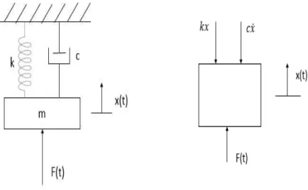
A diagram of a single degree of freedom with an external force 𝐹 (𝑡) is shown on Figure 3.5. The coordinate 𝑥 (𝑡) represents the absolute motion of the mass. It is considered that the external force is harmonic. Applying Newton’s second law, the equation of motion results in (3.30):

𝑚𝑥̈ + 𝑐𝑥̇ + 𝑘𝑥 = 𝐹0sin 𝜔𝑡 (3.30)

(43)

15

This is a nonhomogeneous linear differencial equation. The general solution is given in (3.31).

x(t) = xh(t) + xp(t) (3.31)

The homogeneous solution is represented as x_h(t) wherein are included the free vibrations of the system and the particular solution is represented as x_p(t) which is also called the steady-state solution. The concepts are exposed on Figure 3.6.

Figure 3.6 - Total Response of the System[16]

Using complex algebra and assuming that the response has the same frequency as the force, 𝐹(𝑡) and 𝑥(𝑡) are shown in (3.32).

𝐹(𝑡) = 𝐹0𝑒𝑖𝜔𝑡

𝑥(𝑡) = 𝑋𝑒𝑖𝜔𝑡 (3.32)

Replacing 𝑥 and F on the differential equation of motion results in (3.33):

(−𝑚𝜔2_{+ 𝑖𝑐𝜔 + 𝑘)𝑋𝑒}𝑖𝜔𝑡 _{= 𝐹}

0𝑒𝑖𝜔𝑡 (3.33)

The frequency response function or transfer function, 𝐻(𝜔), is defined as the complex displacement due to a force of unit magnitude, 𝐹₀= 1. Therefore, this function results in (3.34).

𝐻(𝜔) =_{(𝑘 − 𝑚𝜔}1₂_{) + 𝑖𝑐𝜔} (3.34)

The gain function is defined as the modulus of the transfer function in (3.35):

(44)

16

The gain function is the amplitude of the displacement for 𝐹₀= 1 represented in (3.36). 𝑋0

𝐹0 = |𝐻(𝜔)| (3.36)

The frequency ratio is defined in (3.37):

𝑟 = 𝜔

𝜔𝑛 (3.37)

After calculating the modulus of the transfer function, multiplying by k and employing the

definitions for ξ, 𝜔_𝑛 and 𝑐_𝑐 it is possible to obtain the nondimensional gain function in (3.38). 𝑋0

𝐹0⁄ =𝑘

1

√(1 − 𝑟2₎2_{+ (2𝜉𝑟)}2 (3.38)

Figure 3.7 - Gain function for force-excited system[17]

When 𝑟 is close to 1 or when 𝜔 is close to 𝜔_𝑛, the gain function tends to be higher as the damping coefficient is lower. In fact, the response tends to infinite without damping and this phenomenon

(45)

17

3.1.4.2 Base Excitation

Absolute Motion

A diagram of a base-excited system is shown on Figure 3.8. The coordinate 𝑥(𝑡) represents the absolute motion of the mass given the base motion 𝑦(𝑡). From the free-body diagram of Figure 3.8 and applying the Newton’s second law, the equation of motion is represented as (3.39).

𝑚𝑥̈ + 𝑐𝑥̇ + 𝑘𝑥 = 𝑘𝑦 + 𝑐𝑦̇ (3.39)

Figure 3.8 - Base-excited system Assuming that both base motion and response are harmonic in (3.40).

𝑦(𝑡) = 𝑌0𝑒𝑖𝑤𝑡

𝑥(𝑡) = 𝑋𝑒𝑖𝑤𝑡 (3.40)

The transfer function and the gain function are derived in the same manner as for the force-excited

system. The transfer function is expressed in (3.41).

𝐻(𝜔) =_{(𝑘 − 𝑚𝜔}𝑘 + 𝑖𝑐𝜔₂_{) + 𝑖𝑐𝑤} (3.41)

After calculating the modulus of the transfer function and employing the definitions for ξ, 𝜔_𝑛 and 𝑐𝑐 it is possible to obtain the nondimensional gain function in (3.42)

𝑋0

𝑌0 = √

1 + (2𝜉𝑟)2

(1 − 𝑟2₎2_{+ (2𝜉𝑟)}2 (3.42)

The equation above can be also being interpreted as the gain function for acceleration output given

acceleration input. It is actually more common to use it in this form. On Figure 3.9, it is shown

(46)

18

Figure 3.9 - Gain function for base-excited system (absolute displacement)[17]

Relative Motion

Considering the same diagram of a base-excited system shown on Figure 3.8. The coordinate 𝑥(𝑡) represents the absolute motion of the mass given the base motion 𝑦(𝑡). Now the response variable under consideration is the relative displacement in (3.43).

𝑧(𝑡) = 𝑥(𝑡) − 𝑦(𝑡) (3.43)

Thus the new equation of motion is represented in (3.44):

𝑚𝑧̈ + 𝑧̇ + 𝑘𝑧 = −𝑚𝑦̈ (3.44)

Assuming that both base motion and response are harmonic, and following the procedures

described above, the new transfer function is represented in (3.45).

𝐻(𝜔) =_{(𝑘 − 𝑚𝜔}𝑚𝜔₂2_{) + 𝑖𝑐𝑤} (3.45)

The gain function in a nondimensional form is obtained following the procedures described above

and it is represented in (3.46).

𝑍0

𝑌0 =

𝑟2

(47)

19

Figure 3.10 - Gain function for base-excited system (relative displacement)[17]

3.2 Random Vibration Analysis Background

3.2.1 Types of signal

Signals can be classified as stationary or nonstationary. If statistical properties remain constant

with time, the signal is considered to be stationary. Stationary vibration is an idealized concept.

Nevertheless, certain types of random vibration may be regarded as reasonably stationary [18].

On the following flowchart it is presented different stationary types of signal in which is included

stochastic ones, or often called random.

𝑇𝑒𝑠𝑡 𝑆𝑖𝑔𝑛𝑎𝑙 (𝑆𝑡𝑎𝑡𝑖𝑜𝑛𝑎𝑟𝑦)

{

𝐷𝑒𝑡𝑒𝑟𝑚𝑖𝑛𝑖𝑠𝑡𝑖𝑐

{

𝑃𝑒𝑟𝑖𝑜𝑑𝑖𝑐 { 𝑀𝑜𝑛𝑜𝑓𝑟𝑒𝑞𝑢𝑒𝑛𝑡𝑀𝑢𝑙𝑡𝑖𝑓𝑟𝑒𝑞𝑢𝑒𝑛𝑡 𝑃𝑠𝑒𝑢𝑑𝑜 − 𝑠𝑡𝑜𝑐ℎ𝑎𝑠𝑡𝑖𝑐

𝑇𝑟𝑎𝑛𝑠𝑖𝑒𝑛𝑡 {𝑃𝑢𝑙𝑠𝑒 𝑡𝑦𝑝𝑒𝑆𝑡𝑒𝑝 𝑡𝑦𝑝𝑒 𝑆𝑖𝑛𝑒 𝑠𝑤𝑒𝑒𝑝

(48)

20

Table 3.1 gives a practical example of each stationary type signal:

Table 3.1 - Types of stationary signals

Types of Signal Illustration

Mono-frequent time signal

Figure 3.11 - Mono-frequent time signal

Multi-frequent time signal (Time vs. Amplitude)

Figure 3.12 - Multi-frequent time signal

Pseudo-stochastic

Figure 3.13 - Pseudo-stochastic[19]

Pulse type time signal

Figure 3.14 - Pulse type time signal

Step type time signal

Figure 3.15 - Step type time signal

Sine sweep time signal

(49)

21

Types of Signal Illustration

White noise (frequency domain)

Figure 3.17 - White noise (frequency domain)

Broad-band (frequency domain)

Figure 3.18 - Broad-band (frequency domain)

Narrow-band (frequency domain)

Figure 3.19 -Narrow-band (frequency domain)

3.2.2 Random vibration

Random vibration analysis is probabilistic in nature because both input and output quantities

represent only the probability that they take on certain values. Thus, it is not possible to express

its amplitude in terms of a deterministic mathematical function.

Random vibration can be broadband or narrowband. The difference between them is the range of

frequencies contained in the signal. Narrow-banded signals contain only a narrow range of

frequencies, whereas broad-banded signals contain a wide range of frequencies. A white-noise

signal is a special case which implies that the time signal comprises a whole series of harmonics

with exactly the same amplitude, but with purely random phase angles.

The most obvious characteristic of random vibration is that it is no periodic. A knowledge of the

past history of random motion is adequate to predict the probability of occurrence of various

acceleration and displacement magnitudes, but it is not sufficient to predict the precise magnitude

at a specific instant [21].

Frequency PSD

(50)

22

Figure 3.20 - Deterministic and Random Excitation [22]

Random vibration is a varying waveform whereas sinusoidal or harmonic vibration occurs at

distinct frequencies, in other words random vibration contains all frequencies simultaneously.

However random and sine vibration testing cannot be directly compared.

In the past, most vibration was characterized in terms of sinusoids. Nowadays, most vibration is

correctly understood to be random in nature and because of that it is the best way to characterize

them.

Table 3.2- Differences between sinusoidal and random vibration

One of the purposes of using random vibration tests in industry is to prevent failures. The desire

is to find out how a particular equipment may fail because of multiple environmental vibrations

it may encounter. Testing the equipment to failure provides important information about its design

weaknesses and ways to improve it. Random vibration is more realistic than sinusoidal vibration

testing because random simultaneously includes all the forcing frequencies and simultaneously

excites all the equipment resonances. Under a sinusoidal test, a particular resonance frequency

might be found for one part of the device under test and at a different frequency another one may

resonate. Arriving at separate resonance frequencies at different times may not cause any kind of

failure, but when both resonance frequencies are excited at the same time, a failure may occur.

Random testing will cause both resonances to be excited at same time, because all frequency

components in the testing range will be present at the same time [23]. This is one of the big

advantages of random vibration testing.

Harmonical Vibration Random Vibration

- Oscillation - Oscillation

- Predictable - Unpredictable Instantaneous Magnitudes

- Single Frequency - All Frequencies at Once

- Pure Tone/Motion - Statistics

- Spectral Density

(51)

23

Figure 3.21- Random and Sine Waves[24]

In order to clarify the concept of spectrum, the idea can be explained by an experimental test.

According to the experience shown on Figure 3.22 a white light passed through a prism produces

a spectrum of colors. Analogously a random vibration test excites all the frequencies in a defined

spectrum at any given time. So random vibration resembles to white light and sinusoidal vibration

resembles to a one colored laser beam. Another analogy, this one applied in music, can be clarified

in order to simplify the concept. Playing a single piano key produces sinusoidal vibration, on

other hand playing all the piano keys simultaneously produces a signal which approximates

random vibration.

Figure 3.22- White Light Passed Through a Prism

Fig 2.23 has the purpose of clarifying the white light analogy by dividing the random signal

represented as the white light in multiple constant frequency signals represented as different

(52)

24

Figure 3.23 - Random vibration signal analogy with white light

Even though random time signals are not periodic their amplitude spectrum show that time signals

are statistically stationary. This means the statistics of the signal does not change through time.

Another assumption is that the random signal is assumed to be ergodic, this means we could take

a sample across a large set of similar signals at a given time, and expect to get the same mean

value and standard deviation. It was proven that measuring gusting wind loads on a wind turbine

at equal periods of time, all time signals were different in time domain. However, Power Spectral

Density (PSD) plots in frequency domain were identical [25].

3.2.3 Gaussian distribution

It is assumed that the random signal follows a Gaussian distribution. The probability density

function of a Gaussian distribution is calculated from the following equation whereas 𝑥 is a continuous random variable, 𝑋̅ is the mean and 𝜎 is the standard deviation. The standard deviation and the mean vary with time for a nonstationary process but are constant for a stationary one.

Even though random time signals are not periodic their amplitude spectrum show that time signals

are statistically stationary. This means the statistics of the signal does not change through time. A

study carried out by Hafpenny [26] shows that measuring gusting wind loads on a wind turbine

at equal periods of time, all time signals were different in time domain and the plots in frequency

domain were very similar. Thus, random vibration is assumed to be a stationary process that

follows a Gaussian distribution in (3.47).

𝑝(𝑥) = 1 𝜎√2𝜋𝑒−12(

𝑥−𝑋̅ 𝜎 )

2

(53)

25

The curve of the Gaussian distribution has the bell-shaped shown on Figure 3.24:

Figure 3.24 - Gaussian distribution [27]

Since random vibrations theory is based on the probability density function (PDF) of a Gaussian

process, it is important to understand its statistical properties. Random vibration analysis is purely

probabilistic, so both input and output quantities represent only the probability that they take on

certain values. In the last chapter of this dissertation the results in terms of displacement, velocity

and acceleration will be presented as 𝜎-values. These values represent the amplitude of the signal, on the following Table 3.3 and Table 3.4 are shown the probabilities of those random amplitudes.

Table 3.3 - Probability of random amplitudes (1)

Statement Probability Ratio Percent Probability

− σ < x < + σ 0.6827 68.27%

−2 σ < x < + 2 σ 0.9545 95.45%

−3 σ < x < + 3 σ 0.9973 99.73%

Table 3.4 - Probability of random amplitudes (2)

Statement Probability Ratio Percent Probability

|𝑥| > 1 σ 0.3173 31.73%

|𝑥| > 2 σ 0.0455 4.55%

(54)

26

3.2.4 Statistical Properties of Random Vibration

The following paragraphs are referred to statistical properties applied in random vibration

analyses. It is important to understand how the root mean square value is related to the standard

deviation of random signals [28].

The mean square value 𝑋̅̅̅̅2 can be determined from a time history signal 𝑥(𝑡). 𝑥(𝑡) is a generic signal and it can represent displacement, velocity or acceleration. The duration of the time history

is represented as 𝑇. The mean square value can be computed for either continuous or discrete signals by the following equations (3.48) and (3.49), respectively.

𝑋2

̅̅̅̅ = lim_𝑇→∞_{𝑇 ∫}1 [𝑥(𝑡)]2 𝑇

0

𝑑𝑡 (3.48)

𝑋2

̅̅̅̅ = lim_𝑁→∞_{𝑁 ∑ 𝑥}1 𝑖2 𝑁

𝑖

(3.49)

The Root Mean Square (RMS) value is simply the square root of the mean square value, as

represented in (3.50).

𝑅𝑀𝑆 = √𝑋̅̅̅̅2 (3.50)

The fluctuation about the mean value is described by the variance represented as 𝜎2. The standard deviation is represented as 𝜎. The mean value is represented as 𝑋̅. Variance can be calculated for either continuous or discrete signals by the equations (3.51) and (3.52), respectively.

𝜎2 _{= lim} 𝑇→∞

1

𝑇 ∫[𝑥(𝑡) − 𝑋̅]2

𝑇

0

𝑑𝑡 (3.51)

𝜎2_{= lim} 𝑁→∞

1

𝑁 ∑(𝑥𝑖− 𝑋̅)2

𝑁

𝑖

(3.52)

From the equations (3.51) and (3.52) it is possible to deduce the following relationship in (3.53).

𝑋2

̅̅̅̅ = 𝜎2_{+ 𝑋̅}2 _(3.53)

Assuming that random signals have a mean value equal to zero, it is possible to obtain (3.54).

⟹ 𝑅𝑀𝑆 = 𝜎 (3.54)

In order to clarify the concepts, concluding remarks are explained in this paragraph. A random

(55)

27

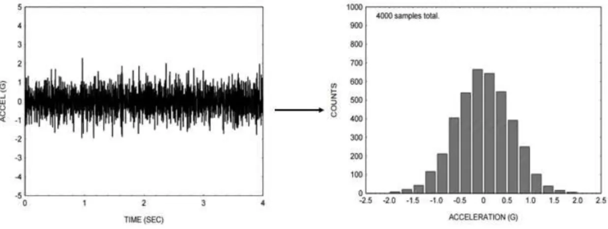
histogram of a random signal converges to a Gaussian distribution as n tends to infinitive. The histogram in Figure 3.25 - Transformation of a time signal in a histogram shows that the random vibration signal has a tendency to remain near its mean value, which in this case is zero. Random

vibrations are expressed in terms of probability of occurrence. Figure 3.25 - Transformation of a time signal in a histogram shows a white noise random signal converted into a histogram. In this figure, x represents acceleration expressed in g unit. This unit is obtained by dividing a signal representing acceleration and expressed in m s⁄ 2 by 9.81.

Figure 3.25 - Transformation of a time signal in a histogram

This histogram can be converted to a probability density function by dividing each bar by the total

number of samples. The resulting probability density function is an approximated Gaussian

density function. [18] Considering that random vibration theory is based on the assumption that

the signal follows a Gaussian distribution, it is possible to determine the probability that an

amplitude will occur inside or outside certain limits. Thus, considering these statistical properties

and assumptions, the root-mean-square value is equal to the standard deviation as shown in Figure

3.26.

(56)

28

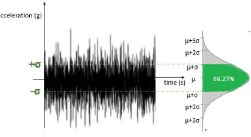
As a concluding remark, Figure 3.27 simplifies the statistical properties of a random vibration

signal in time domain assumed as stationary and ergodic.

Figure 3.27 - Statistical Properties of a Random Vibration Signal

3.2.5 How to calculate PSD

Time histories can be represented in the frequency domain in different formats. Power Spectral

Density (PSD) is the most effective format to analyze random vibration. A PSD analysis is a

sophisticated and extremely useful form to measure vibration. PSD functions may be calculated

via three distinct methods.

The first one is based on measuring the RMS value of the amplitude in successive frequency

bands, where the signal in each band has been bandpass filtered. This technique used by electrical

engineers near the year of 1940 actually generated what nowadays is known by PSD functions.

They were interested to see the amplitude spectrum based on measured randomly varying signals

[17]. Since digital acquisition system had not been invented yet, they had to invent a procedure

using analog filters. The waveform was iteratively filtered to a signal with only a single frequency.

The filtered signal’s mean-square value was then measured and plotted. This was called the ‘power’ at that frequency. However, in practice, it is impossible to produce a physical filter that outputs only a single frequency; the output is actually a signal which is dominated within a narrow

bandwidth ∆𝑓. The PSD gets his name from the fact that these electrical engineers who invented this technique were interested in electrical power, plotting a spectrum of frequencies and

(57)

29

Figure 3.28 - Spectral analysis procedure using analog filters

However, this plot of Power is ambiguous. It was proven by Wayne Tustin [29] that the bandwidth

influences the Power in 𝑔2 units. The measured power was divided by the bandwidth ∆𝑓 to cancel its influence on data producing the units of 𝑢𝑛𝑖𝑡𝑠2⁄𝐻𝑧.

It was extremely important to normalize data in order to quantify vibration levels with a unique

and standard unit of measurement. The reason why vibration unit of measurement is 𝑔2⁄𝐻𝑧 is explained with a practical example which was performed in a laboratory.

For this experimental test, it was needed an accelerometer attached to a small electrodynamic

shaker and suitable signal conditioner, a band-pass filter and a true RMS readout voltmeter.

The results of a filtered signal measurement with a center frequency (fc) of 1000 Hz and several

bandwidths are shown on Table 3.5:

(58)

30

It was concluded that when measuring the exact same signal with 𝑔2 units, the results were not uniform. It was desirable to normalize data to a common value to compensate the difference of

the analyzer bandwidth, thus eliminating ambiguity. This unit of 𝒈_𝑹𝑴𝑺𝟐⁄𝑯𝒛 is nowadays the standard unit to measure vibration and it also is the unit used for quantify Power Spectral Density,

in this specific case for Acceleration Spectral Density. The standard unit to quantify Displacement

Spectral Density is 𝑚𝑚2⁄𝐻𝑧 and to quantify Velocity Spectral Density is (𝑚𝑚

𝑠 )

2

𝐻𝑧 ⁄ .

Figure 3.29 - Calculation of a Power Spectral Density in a standardized unit of measure

There are two advantages of measuring the signal in this way: the bandwidth of the filter does not

influence the level of power spectral density and due to the statistical properties and assumptions

of the random signal, the area under the spectral density function is equal to the root mean square

of the waveform.

Therefore, it is possible to quantify and analyze random vibration. Using this method, various

laboratories, firms, and agencies can communicate regarding random vibration intensity.

Nowadays this method of obtaining PSD is not used very often, it is more usual to take advantage

of computers to calculate the PSD plot directly from digitized time signals. In this analysis, it is

applied the Fast Fourier Transform algorithm. In the Appendix A, it is presented the Fourier

Transform background. The PSD is calculated from the technique shown on the following

(59)

31

Figure 3.30 - PSD calculation technique

Firstly, it is performed the FFT to the time signal waveform decomposing it into its constituent

harmonics described in terms of amplitude, frequency and phase. The Amplitude Spectrum which

is a plot of amplitude vs. frequency is obtained after calculating the modulus of the complex

numbers. The Power Spectrum is obtained by squaring the amplitude spectrum. Finally, dividing

by 2 times the duration of the time signal in seconds it is obtained the PSD which, actually

represents the density function of the mean of the amplitude-squared spectrum. In the Appendix

A, the Fourier Transform background is comprehensively explained.

There is another method to obtain PSD which is based on taking the Fourier transform of the

autocorrelation function. This technique is more theoretical and it is known as the

Wierner-Khintchine Theorem [30].

3.2.6 The meaning of

𝒈

_𝑹𝑴𝑺

in sine and random vibration

The need to use material that was developed to harmonic, also referred as sine by the Military

Standard [31], requirements has generated a demand to understand and to determine equivalence

between sine and random vibration. A general definition of equivalence is not feasible since both

characterizations of vibration are based on distinctly different sets of mathematics. The details of

material dynamic response have to be known in order to compare the effects of given random and

sine vibration on material.

Despite dimensional units are quantified as typically acceleration in standard gravity (𝑔) on both tests, these are not equivalent and cannot be directly compared. Peak acceleration of sine

measured in 𝑔 is not equivalent to the result measured in 𝑔 of a random test, soboth values of 𝑔𝑅𝑀𝑆 are also not comparable. On one hand, 𝑔𝑅𝑀𝑆 sine acceleration is the root mean square of a

time signal at one specific frequency. On the other hand, random 𝑔_𝑅𝑀𝑆 is the square root of the area under the spectral density curve including all frequencies simultaneously.

𝐹𝐹𝑇 |𝐹𝐹𝑇| |𝐹𝐹𝑇|2 _{𝑃𝑆𝐷 =} 1

(60)

32

Figure 3.31 – grms on a sine test

Figure 3.32 – grms on random test

3.2.7 Dynamic analysis

The dynamic analysis methodology is based on three stages as shown on Figure 3.33:

Figure 3.33 - Dynamic Analysis Methodology

The purpose of carrying out a modal analysis is to obtain the natural frequencies and normal

modes of vibration of the structure. Considering the equation of motion in the absence of applied

external forces and damping in (3.55).

(61)

33

And assuming a sinusoidal response wherein 𝑥̅ represents the amplitude of the sinusoidal vibration in equations (3.56).

{ 𝜈 = 𝑥̇ = 𝑥̅𝜔 cos 𝜔𝑡𝑥 = 𝑥̅ sin 𝜔𝑡

𝑎 = 𝑥̈ = −𝑥̅𝜔2_{sin 𝜔𝑡} (3.56)

Replacing the sinusoidal response in the equation of motion (3.55):

(−𝜔2_{[𝑀]𝑥̅ + [𝐾]𝑥̅) sin(𝑤𝑡) = 0}

⇒ (−𝜔2_{[𝑀] + [𝐾])𝑥̅ = 0} (3.57)

Equation (3.57) represents the formulation of a generalized eigenproblem. The natural

frequencies are represented by the eigenvalues and the normal modes of vibration are represented

by the eigenvectors.

Figure 3.34 - Eigenvalues solution

The frequency response analysis is carried out by exciting the structure with a unit of acceleration

over frequency range using the saved eigenvalues. This excitation is similar to a Dirac Impulse in

time domain. This excitation generates the transfer function, 𝐻_𝑓.

Figure 3.35 - Transfer Function 𝐻_𝑓.

The random response analysis is essentially a post processing exercise on the frequency response

analysis. The PSD response is obtained from the PSD input and the transfer function calculated

from the previous stage trough equation (3.58).