Essays on multi-country economic growth and sectoral total factor productivity

(1)

FUNDAÇÃO GETÚLIO VARGAS

ESCOLA DE PÓS-GRADUAÇÃO EM ECONOMIA

Mariana Fialho Ferreira

Essays on Multi-Country Economic

Growth and Sectoral Total Factor

Productivity

Rio de Janeiro 2016

(2)

Essays on Multi-Country Economic

Growth and Sectoral Total Factor

Productivity

Tese submetida à Escola de

Pós-Graduação em Economia como requisito parcial para obtenção do grau de Doutor em Economia

Área de concentração: Desenvolvimento Orientador: Pedro Cavalcanti Gomes Fer-reira

Co-orientador: João Victor Issler

Rio de Janeiro 2016

(3)

Ficha catalográfica elaborada pela Biblioteca Mario Henrique Simonsen/FGV

Ferreira, Mariana Fialho

Essays on multi-country economic growth and sectoral total factor productivity / Mariana Fialho Ferreira. – 2016.

182 f.

Tese (doutorado) - Fundação Getulio Vargas, Escola de Pós- Graduação em Economia.

Orientador: Pedro Cavalcanti Gomes Ferreira. Coorientador: João Victor Issler. Inclui bibliografia.

1. Desenvolvimento econômico. 2. Produtividade. I. Ferreira, Pedro Cavalcanti. II. Issler, João Victor. III. Fundação Getulio Vargas. Escola de Pós-Graduação em Economia. IV. Título.

CDD – 338.9

(4)

(5)

(6)

e estudo, mas, sobretudo, o empenho daqueles que sempre torceram pelo meu sucesso e con-tribuíram de forma imensurável para o meu engrandecimento pessoal e pro…ssional.

Em primeiro lugar, gostaria de agradecer aos meus pais, Ana Teresa e Antonio Augusto, por fazerem dos meus sonhos os deles, e não pouparem esforços para que se tornassem realidade. Muito obrigada por nunca me permitirem duvidar de que eu seria capaz de alcançar tudo aquilo que almejasse. Por estarem sempre presentes na minha vida, tanto nas horas mais difíceis como nas de comemorações. Meu amor por vocês é incondicional.

Ao meu esposo, Patrick, que ao longo do doutorado foi meu namorado, meu noivo, meu melhor amigo, meu porto seguro, meu amor. Obrigada por ser tão generoso e compreensivo. Não tenho palavras para agradecer a leveza que você trouxe para a minha vida. É por você que acordo todos os dias com a certeza de que estou no lugar certo, na hora certa. E é para você que eu tento me tornar um ser humano melhor.

À Dixie, por me ajudar a arejar a mente, obrigando-me a fazer pausas; nem sempre progra-madas, mas exigidas pelo mais puro olhar que existe.

Ao meu irmão, Pedro Henrique, por permitir que nossas discussões …losó…cas madrugadas adentro não fossem afetadas pela distância ou pelo tempo. Não há absolutamente nada no mundo que eu não faria por você.

À minha avó e madrinha Léa, meu exemplo de determinação, força e resiliência. Ao tios Lauro Jair e Vera, por terem me acolhido com tanto carinho assim que cheguei ao Rio.

Aos irmãos que o doutorado me trouxe, Júlia Fonseca, Mariana Milhomem, Fernanda Jardim e Victor Duarte, meus fantásticos companheiros ao longo desta maratona, desde a largada. Obrigada por serem a mão amiga com a qual eu tinha a certeza de poder contar em qualquer circustância, tempo e lugar. Minha jornada teria sido absurdamente mais pesada sem a amizade e o carinho de vocês.

Aos amigos de Vitória, Luciana Cazoto, Marcos Guimarães, Vanessa Rozindo, Carol Berger, Victor Passos e Saulo Pratti, pela paciência em cultivar nosso convívio à distância a cada dia, sem deixá-lo esmorecer. Às amigas do Rio, Renata Moraes e Cinthya Bretz, por aceitarem fazer parte da minha família em terras cariocas, também composta pelos primos Alexandre e Joanna Terezan.

Aos estimados professores Rogério Arthmar e Robson Grassi (UFES), por terem feito nascer em mim a paixão pelas Ciências Econômicas, e Victor Gomes e Roberto Ellery (UnB), por me mostrarem o quão fascinante pode ser a pesquisa em Macroeconomia e, especialmente, em Crescimento Econômico.

Ao meu orientador Pedro Cavalcanti e co-orientador João Victor Issler (EPGE-FGV), agradeço imensamente toda a con…ança que depositaram em mim, as horas de intensa dedicação à minha formação e ao trabalho que realizamos em conjunto e a exigência e incentivo com que o con-duziram, os quais foram fundamentais para que eu me tornasse uma pesquisadora cada vez mais segura. Aos demais professores da Congregação da EPGE, por todos os ensinamentos transmitidos, dentro e fora de sala de aula. A convivência com cada um foi extremamente en-riquecedora e singular. Aos demais funcionários da Escola, deixo também o meu muito obrigado pelo incomparável pro…ssionalismo e sensibilidade, demonstrados a todo momento.

Agradeço, por …m, o apoio a mim concedido pela Fundação Getúlio Vargas e, em especial, pela Escola de Pós-Graduação em Economia. Foi uma verdadeira honra ter sido aluna dessa conceituada e tradicional Escola. Ao mesmo tempo, foi também uma grande satisfação pessoal ter aceitado este desa…o que, como tal, envolveu inúmeros momentos de alegria e de renúncia, sempre acompanhados, contudo, pela absoluta certeza de que não havia caminho alternativo a ser seguido, que não o da excelência.

(7)

"For life is quite absurd And death’s the …nal word You must always face the curtain with a bow Forget about your sin - give the audience a grin Enjoy it - it’s your last chance anyhow"

Always Look on the Bright Side of Life Monty Python’s Life of Brian

(8)

Nesta tese, oferecemos uma abordagem alternativa - e talvez mais apropriada - para a estimação da produtividade total dos fatores (PTF) setorial. Nossa economia arti…cial utiliza insumos produzidos por diferentes setores para produzir cada um dos bens, os quais, por sua vez, podem ser empregados como insumo ou consumidos pelo agente representativo em um arcabouço de equilíbrio geral. Essa estrutura de insumo-produto é adequada a uma ampla gama de exercícios, que podem ser desenvolvidos usando bases de dados que foram disponibilizadas apenas recen-temente. No primeiro capítulo, construímos séries em nível e índices de produtividade para 35 atividades e 40 países, que respondem por mais de 85% do PIB mundial, e séries agregadas para países e para os 3 setores da economia. Nossos resultados sugerem que, na maioria dos países, o setor de serviços não apenas apresentou produtividade mais alta do que a indústria, mas também que a diferença de produtividade entre esses dois setores está aumentando com o passar do tempo. Esses resultados vão de encontro a algumas conclusões amplamente conheci-das, as quais foram elaboradas a partir de dados sobre a produtividade do trabalho. Isso ocorre principalmente pelo fato de a nossa abordagem possibilitar a mensuração da in‡uência de todos os insumos produtivos sobre a produtividade total dos fatores. No capítulo 2, nós buscamos avaliar a importância quantitativa dos cost shares setoriais para o crescimento da produtividade setorial e agregada. Para tanto, realizamos uma análise comparativa relacionando as taxas de crescimento da PTF setoriais e agregadas dos EUA e do Brasil, e conduzimos dois conjuntos de exercícios contrafactuais. O principal propósito desses execícios é avaliar em que medida mu-danças nos cost shares associados com o uso intermediário de produtos afetam o crescimento da produtividade setorial e agregada. A partir do primeiro conjunto de exercícios, concluímos que os melhores resultados - em termos de elevações no crescimento da PTF - parecem ser alcança-dos quando substituímos as participações da indústria doméstica brasileira no custo total de sua indústria pelos cost shares norte-americanos correspondentes, uma vez que elas são capazes de melhorar a PTF em um maior número de atividades e, consequentemente, estimular as taxas de crescimento da produtividade em todos os três setores e no agregado da economia. A partir do segundo conjunto de contrafactuais, concluímos que a escolha ótima de fornecedores estrangeiros, assim como o trade-o¤ entre insumos domésticos e importados, como prescritos pelo modelo, são consistentes com um cenário de produtividade mais próspero. O capítulo 3 investiga os principais determinantes do crescimento econômico da América Latina e Caribe (LAC), levando em conta alterações no ambiente econômico da última década e contrastando a importância rel-ativa de condições externas favoráveis com a de políticas públicas adequadas. Nós estimamos a equação de crescimento utilizando estimadores de métodos de momentos generalizados (GMM) desenvolvidos para modelos dinâmicos de dados em painel e, a partir dos coe…cientes estimados, investigamos a contribuição de cada um dos grupos de determinantes para a variação esper-ada do crescimento econômico. Por …m, conduzimos um exercício contrafactual, objetivando quanti…car em que medida os termos de troca favoráveis foram responsáveis pelo crescimento econômico recente da região da LAC. Nós concluímos que essa variável foi, de fato, um deter-minante signi…cativo para o crescimento econômico dos países latino-americanos ao longo da década passada.

(9)

Abstract

In this thesis, we o¤er an alternative - and perhaps more appropriate - analytical setup for estimating sectoral total factor productivity (TFP). The arti…cial economy uses inputs from di¤erent sectors in producing every commodity, which is either used as an input or consumed by the representative agent in a general equilibrium framework. This input-output structure is suitable for a wide range of exercises, which can be performed using datasets that only recently became available. In the …rst chapter, we construct 35-activity TFP indices and level series for a group of 40 countries, which responds for more than 85% of world GDP, and aggregate data to construct country-level and 3-sector indices and level series. Our …ndings suggest that, in most of the countries, the services sector not only has presented higher productivity than industry, but also that these di¤erences are getting larger over time. These results are at odds with some widely known conclusions, which have been drawn from labor productivity data by previous work in the …eld. It occurs mainly because our framework enables us to quantify the in‡uence of all productive inputs on total factor productivities. In chapter 2, we aim to evaluate the quantitative importance of sectoral cost shares in explaining sectoral and aggregate productivity growth. To this end, we perform a comparative analysis concerning sectoral and country-level TFP growth rates in the USA and in Brazil and conduct two sets of counterfactual exercises. The main purpose of these exercises is to assess to what extent changes in the cost shares associated with intermediate uses of outputs a¤ect sectoral and aggregate total factor productivity growth. As a result of the …rst set of exercises, we …nd that the best outcomes - in terms of enhancing TFP growth - seem to be achieved when we replace Brazil’s shares of its domestic industry in the total cost of its industry by the corresponding cost shares of the US economy, since they are able to improve TFP in a higher number of activities and, as a result, to boost TFP growth rates in all three sectors and in total economy. From the second set of counterfactuals, we conclude that the optimum choice of international suppliers, as well as the trade-o¤ between domestic and imported inputs, as prescript by the model, are consistent with a more ‡ourishing productivity scenario. Chapter 3 investigates the main determinants of economic growth in Latin America and the Caribbean (LAC), considering changes on last decade’s economic environment and measuring the relative importance of favorable external conditions and of proper public policies. We estimate a growth equation using generalized method of moments (GMM) estimators designed for dynamic models of panel data and, from the estimated coe¢ cients, we assess the contribution of each group of determinants to expected change on economic growth rates. At last, we conduct a counterfactual exercise, aiming to evaluate to what extent enabling terms of trade were responsible for recent LAC’s economic growth. We …nd that this variable was, indeed, a signi…cant determinant for latin american countries’economic growth over the last decade.

(10)

1.1 Country-level Aggregate TFP Index - Selected Countries . . . 29

1.2 Annualized Growth Rates of TFP: Agriculture vs. Total Economy . . . 30

1.3 Annualized Growth Rates of TFP: Industry vs. Total Economy . . . 31

1.4 Annualized Growth Rates of TFP: Services vs. Total Economy . . . 32

1.5 Relative Total Factor Productivity: Services-Industry Ratio for Forty Economies in 1996. . . 33

1.7 Multi-Country 3-Sector TFP Levels - Selected Countries . . . 35

1.8 TFP Level Series: Brazil - Selected Activities . . . 37

1.9 TFP Level Series: Brazil - Real Estate Activities . . . 38

1.10 TFP Level Series: China - Selected Activities . . . 39

1.11 TFP Level Series: Japan - Selected Activities . . . 40

1.12 TFP Level Series: Netherlands - Selected Activities. . . 41

1.13 TFP Level Series: Netherlands - Mining and Quarrying . . . 41

1.14 TFP Level Series: the UK - Selected Activities . . . 42

1.15 TFP Level Series: the USA - Selected Activities. . . 43

1.16 Country-level Aggregate TFP Index - Euro-Zone Selected Countries . . . 51

1.17 Country-level Aggregate TFP Index - Non-Euro EU Selected Countries . . . 52

1.18 Country-level Aggregate TFP Index - Other Selected Countries . . . 52

1.19 Country-level Aggregate TFP Levels - Selected Countries . . . 53

1.20 Country-level Aggregate TFP Levels - Euro-Zone Selected Countries . . . 54

1.21 Country-level Aggregate TFP Levels - Non-Euro EU Selected Countries . . . 54

1.22 Country-level Aggregate TFP Levels - Other Selected Countries. . . 55

1.23 3-Sector TFP Levels - Industry displaying low relative TFP . . . 56

1.24 3-Sector TFP Levels - Agriculture displaying low relative TFP . . . 57

1.25 3-Sector TFP Levels - Services displaying low relative TFP . . . 57

1.26 3-Sector TFP Levels - Services displaying high relative TFP - Group 1 . . . 58

1.27 3-Sector TFP Levels - Services displaying high relative TFP - Group 2 . . . 59

1.28 3-Sector TFP Levels - Industry displaying high relative TFP . . . 59

1.29 3-Sector TFP Levels - Agriculture displaying high relative TFP . . . 60

2.1 Annualized Growth Rates of TFP: Agriculture vs. Total Economy . . . 73

2.2 Annualized Growth Rates of TFP: Industry vs. Total Economy . . . 73

2.3 Annualized Growth Rates of TFP: Services vs. Total Economy . . . 74

2.6 Multi-Country 3-Sector TFP Levels - Selected Countries . . . 76

2.7 TFP Level Series: Brazil - Selected Activities . . . 78

(11)

2.9 TFP Level Series: the USA - Selected Activities. . . 80

2.10 TFP Index: Total Economy - BRA vs. USA. . . 81

2.11 TFP Sectoral Indices: BRA vs. USA . . . 82

2.12 Annualized growth rates of TFP in Brazil’s 35 activities/3 sectors/total economy in the model and in the counterfactual C1.1 . . . 93

2.15 Annualized growth rates of TFP in Brazil’s 35 activities/3 sectors/total economy in the model and in the counterfactual C2 . . . 107

3.1 PIB per capita real de países selecionados da LAC . . . 136

3.2 Taxas de Crescimento do PIB per capita, por região e por década - 1961-2010 . . 137

3.3 Taxas de Crescimento do PIB per capita, por região e por década - 1961-2010 . 138 3.4 Taxas de Crescimento do PIB per capita, - América Latina e Países Selecionados 140 3.5 Taxas de Crescimento do PIB per capita: Cone Sul . . . 141

3.6 Taxas de Crescimento do PIB per capita: Comunidade Andina . . . 142

3.7 Taxas de Crescimento do PIB per capita: América Central . . . 143

3.8 Taxas de Crescimento do PIB per capita: Caribe Continental . . . 144

3.9 Taxas de Crescimento do PIB per capita: Caribe - Grandes Ilhas . . . 145

(12)

1.1 ISIC 3.0 vs. 3-Sector Correspondence. . . 61

2.1 WIOT schematic outline . . . 85

2.2 A matrix schematic outline . . . 87

2.3 Modi…ed A matrix - Counterfactual 1 . . . 89

2.4 Modi…ed WIOT - Counterfactual 1 . . . 90

2.5 Counterfactual’s guide . . . 92

2.6 Annualized growth rates of TFP in Brazil’s economic activities - C1.1 . . . 95

2.7 Capital and labor intensities in Brazil’s economic activities - C1.1 . . . 96

2.8 Annualized growth rates of TFP and capital/labor intensities in Brazil’s 3 sectors and total - C1.1 . . . 96

2.11 Annualized growth rates of TFP and capital/labor intensities in Brazil’s 3 sectors and total - C1.2. . . 99

2.15 Modi…ed A matrix - Counterfactual 2 . . . 104

2.16 Modi…ed WIOT - Counterfactual 2 . . . 105

2.17 ISIC 3.0 vs. 3-Sector Correspondence. . . 113

2.18 ISIC 3.0 vs. 10-Sector Correspondence . . . 114

(13)

2.33 Annualized growth rates of TFP and capital/labor intensities in Brazil’s 3 sectors

and total - C2.2. . . 125

3.1 Variáveis de Interesse. . . 148

3.2 Regiões e Países. . . 160

3.3 Estatísticas Descritivas Univariadas. . . 161

3.4 Correlações . . . 163

3.5 Resultados da Estimação da Equação de Crescimento . . . 170

3.6 Comparação entre décadas - 2000 vs. 1990. . . 174

3.7 Comparação entre intervalos de cinco anos - 2006-2010 vs. 2001-2005 . . . 176

(14)

1 On Deriving Evidence from Input-Output Linkages: A Multi-Country

Sec-toral Total Factor Productivity Analysis 16

1.1 Introduction. . . 16

1.2 The Model . . . 18

1.2.1 Dynamic General Equilibrium: Open Economy Setup . . . 18

1.2.2 Economic Environment . . . 19

1.3 Data and identi…cation strategy. . . 24

1.3.1 Data . . . 24

1.3.2 Identifying the series’components . . . 25

1.4 Multi-Country Sectoral Total Factor Productivity Series . . . 28

1.4.1 3-Sector and Country-level Aggregation . . . 28

1.4.2 Multi-Country Aggregate TFP Indices . . . 28

1.4.3 Multi-Country 3-Sector Growth Rates of TFP . . . 29

1.4.4 Multi-Country 3-Sector TFP Levels . . . 32

1.4.5 Multi-Country 35-Activities TFP Levels . . . 36

1.5 Conclusions . . . 43

References . . . 44

Appendix 1 . . . 47

Appendix 2 . . . 51

Appendix 3 . . . 56

2 Assessing the Quantitative Importance of Sectoral Cost Shares for Total Fac-tor Productivity Growth 62 2.1 Introduction. . . 62

2.2 The Model . . . 64

2.2.1 Dynamic General Equilibrium: Open Economy Setup . . . 64

2.2.2 Expected Utility Maximization . . . 66

2.2.3 Optimal Quantities. . . 67

2.2.4 Dynamics . . . 68

2.3 Stylized Facts . . . 69

2.3.1 Data . . . 69

2.3.2 Identifying the series’components . . . 70

2.3.3 Multi-Country3-Sector TFP Growth Rates . . . 72

2.3.4 Multi-Country 3-Sector TFP Levels . . . 74

2.3.5 Multi-Country 35-Activities TFP Levels . . . 77

2.4 Quantitative Analysis . . . 80

2.4.1 Comparing growth rates of TFPs . . . 80

2.4.2 Counterfactuals . . . 83

2.5 Conclusions . . . 108

References . . . 110

(15)

Appendix 2 . . . 115

3 Determinantes do Crescimento Econômico da América Latina 135 3.1 Introdução. . . 135

3.2 Determinantes do Crescimento Econômico . . . 136

3.2.1 Fatos Estilizados . . . 136

3.2.2 Variáveis de Interesse . . . 147

3.3 Estimação e Resultados . . . 159

3.3.1 Amostra e Estatísticas Descritivas . . . 159

3.3.2 Metodologia de Estimação . . . 164

3.3.3 Resultados . . . 168

3.4 Projeções . . . 171

3.4.1 Comparação entre Décadas . . . 171

3.4.2 Comparação entre Períodos de 5 Anos . . . 175

3.4.3 Comparação entre Termos de Troca Fixos e Variáveis . . . 177

3.5 Conclusão . . . 179

(16)

On Deriving Evidence from

Input-Output Linkages: A

Multi-Country Sectoral Total Factor

Productivity Analysis

1.1 Introduction

Over the last decades, a relevant strand of the macroeconomic literature has sought to uncover the sources of di¤erences in income across countries. A substantial number of studies has pointed out the primary importance of cross-country di¤erences on labor productivity and total factor

productivity (TFP)1in explaining large shares of di¤erences in income. Moreover, new branches

of this literature have dedicated great e¤orts to show how sectoral di¤erences in productivity drive the process of reallocation of factors between the many activities of an economy and, ultimately, can account for the aggregate productivity outcomes.

It is relevant to note that there have been some well recognized obstacles posed to this potentially fruitful agenda. For instance, as stressed by Duarte and Restuccia (2015) until the recent release of the World Income-Outcome Database (Timmer, M. P. et al. (2015)), sources of comprehensive sectoral data were scarce.

That said, in order to assess the contribution of sectoral productivity to aggregate out-comes, researchers in the …eld had to rely on expenditure data to establish patterns of sectoral productivity across countries. However, some inferences made from expenditure price data may be misleading.

As argued by Duarte and Restuccia (2010), the conventional wisdom about price-level dif-ferences across country was typically built upon expenditure prices (e.g., from PWT or ICP) instead of producer prices. This led, for example, to the widely spread idea that the relative

prices2 of agriculture and services are higher in rich than in poor countries. By claiming that

food is cheap in poor countries, within this speci…c category of analysis, what is really being stated is that food expenditures are higher in rich countries. However, food expenditures in-clude distribution and other charges so that, depending on the country under scrutiny, it may imply in a signi…cant disparity between these prices and the ones faced by producers. On the other hand, the model of structural transformation proposed by Duarte and Restuccia, which has implications for producer prices, generates diametrically opposed results: the dispersion in productivity across rich and poor countries is larger in agriculture and services relatively to manufacturing, implying that relative prices are higher in poor than in rich countries.

1_{In this paper, we use the expressions "total factor productivity", "TFP"and "productivity"interchangeably.} 2

(17)

17

The World Input-Output Database (WIOD)3 may be described as the most up-to-date and

comprehensive sectoral cross-country database. This brand new database enables a wide range of sectoral studies, as it provides data for 35 economic activities and 40 countries, from 1995 to 2009. Besides compiling a large amount of multilateral data in its World Input-Output Tables (WIOTs), the Socio-Economic Accounts (SEA) also contains disaggregated data on output,

wages and employment and capital stock.4

For our purposes, the most interesting feature of the WIOTs is that they are valued at basic prices, i.e., all values in their intermediate and …nal use blocks represent the amount receivable by the producer from the purchaser. The construction methodology of these tables guarantees that the trade and transport margins cannot interfere in their valuation, as they are recorded

in separate rows.5 In other words, the valuation method adopted ensures that our results are not

going to be dictated by expenditure prices, and thus it secures our conclusions against producing misleading inferences.

Another limitation for quantitative sectoral productivity studies is the fact that, up to the present date, there are no activity-level total factor productivity series available. Even though some estimates of labor productivity for a large set of countries and disaggregated activities

have already been made6, actual data on total factor productivity is not yet available. However,

theory says that total factor productivity is one of the main drivers of cross-country growth. The main reason for the absence of sectoral TFP data is that disaggregated capital stock series are not available for most of the countries. More precisely, o¢ cial sectoral capital stock data is available only up to 2007, and for a very limited set of OCDE countries in the EU KLEMS database. The WIOD computed, also only up to 2007, series for the remaining countries covered by the database on the basis of the Perpetual Inventory Method. To accomplish that, certain assumptions concerning the depreciation rates had to be made and, for those countries whose

investment series were too short, the initial capital stock had to be estimated.7

In this paper, we o¤er an alternative - and perhaps more appropriate - analytical setup for estimating sectoral TFP. We employ the seminal contribution of Long and Plosser (1983) to the real business cycle literature to construct total factor productivity (TFP) measures that are multi-country and multi-sector. This is a novel approach, since the previous literature has used

only labor productivity measures to discuss long-run growth.8

Long and Plosser focused mainly on showing how a simple general equilibrium model, built upon standard assumptions regarding individual’s preferences and production possibilities, was capable of explaining certain business cycle regularities. Subsequent work on the …eld, e.g., Durlauf (1989) and Engle and Issler (1995), worried about the dynamic properties of the data in terms of common trends and common cycles. So far, no one has used the model to construct sectoral TFP measures, something that is lacking in TFP literature.

The arti…cial economy proposed here uses inputs from di¤erent sectors in producing every commodity, which is either used as an input or consumed by the representative household in a general equilibrium framework. This input-output structure is suitable for a wide range of cross-country exercises that can be performed using datasets that only recently became available. In short, by combining worldwide data from the WIOD and the input-output linkages of the model, we are now able to calculate sectoral total factor productivity for a set of countries that respond to more than 85% of world’s GDP. Due to the deepening of the globalization process, it is imperative for the economic growth literature to investigate to what extent global value

3_{Which includes the World Input-Output Tables (WIOTs) and the Socio Economic Accounts (SEA).} 4

Although there are annual WIOTs until 2011, labor data obtainable from SEA is only available for the full set of 40 countries until 2009.

5

See Timmer, M. et al. (2012b).

6_{See Duarte and Restuccia (2010), Duarte and Restuccia (2015) and Inklaar and Timmer (2014)} 7

For more information, see Timmer, M et al. (2012b).

8_{For instance, see Baumol (1967), Baumol et al. (1985), Baumol (1986), McMillan and Rodrik (2011), Rodrik}

(18)

chains are important for a given country’s sectoral productivity and, therefore, for its aggregate outcomes.

We …rst construct 35-activity TFP indices and level series for a group of forty countries. We then aggregate data to construct country-level and 3-sector indices and level series, so that we can extract some new insights and compare our country-level data. Our …ndings suggest that, in most of the countries, the services sector not only has presented higher productivity than industry, but also that these di¤erences are getting larger over time.

In fact, our results are at odds with some widely known conclusions, which have been drawn from labor productivity data by previous work in the …eld. It occurs mainly because our model enables us to quantify the in‡uence of all productive inputs over total factor productivities.

This paper is organized as follows. In the next section, we present the model that theoretically supports our subsequent accounting exercises. In Section 3, we describe the database adopted for our quantitative analysis, the identi…cation strategy we chose to apply and the main steps for the computation of the TFP level series for the 35 economic activities, for the 3 sector aggregation and for the country-level aggregation. Section 4 provides the main results. Section 5 concludes.

1.2 The Model

1.2.1 Dynamic General Equilibrium: Open Economy Setup

In this section, we present the framework that gives support to our empirical analysis. We closely follow the real business cycle setup proposed by Long and Plosser (1983), but we implement some adjustments in order to match an environment that contains many heterogeneous open

economies.9

Due to the increasing globalization of value chains, there is a growing number of goods and services that are no longer produced within a single country. Therefore, to capture the impacts of international trade of goods and services over each sector, we assume that there are C countries in our economic environment, in which I di¤erent industries operate.

The individual who solves the maximization problem that will be described in the following sections thus may have to consider the allocation of up to N = I C commodities. In other words, an activity i, i 2 f1; 2; :::; Ig, whose production is specialized in one single sort of commodity, may have up to C di¤erent "plants"producing it, each of them based in one of the C countries. The commodities’ characteristics thus have two important dimensions. First, they di¤er

in their own "nature", e.g., one of the produced commodities may be labelled as "textiles

and textile products", belonging to the wider group "manufacturing", and another one may be assigned to "hotels and restaurants", belonging to "services". Second, they can be domestically produced or imported from other countries.

Therefore, when deciding which inputs to employ in a given production process, or when establishing his consumer basket for the period, the agent have to take into account the allocation both the domestically produced commodities and the ones produced abroad.

The timing of the events in this economy can be described as follows: at the beginning of each period, the individual chooses (i) his consumption plan, i.e., the commodity bundle and the amount of leisure (in time units) he is willing to consume during the period and (ii) his production plan, i.e., quantities of all commodities and labor (in time units) inputs to be allocated in every productive transformation that takes place (and it is concluded) during the period.

During every period, various random shocks modify the productive transformations, although they cannot in‡uence the individual’s tastes. Thus, the total commodity stocks that will be

9

(19)

19

available at the beginning of the subsequent period are derived from the combined result of the input choices made at the beginning of the current period and the random shocks to the production activities that occur along the period.

1.2.2 Economic Environment

Preferences

The model’s economy has a single in…nite-lived individual (or a constant number of identical individuals), endowed with initial resources, production possibilities and preferences. The indi-vidual then has to choose, based on his marginal rate of substitution, a preferred

consumption-production plan.10 The economic activities in this environment may be summarized as repetitions

of one-period cycle, each of them beginning with this individual’s choice problem (or, similarly, the representative agent’s problem).

At the beginning of the period the individual chooses a consumption-production plan that maximizes the value of his expected discounted utility, constrained by the availability of resources and the production possibilities. At t = 0, the individual’s utility U is given by:

U = 1 X t=0 t_u(C t; Zt); 0 < < 1 (1.1)

where is a discount factor, Ct is a N -vector of commodity consumption at time t, and Zt

is the total amount of leisure (measured in time units) consumed in period t. As we can clearly

notice from equation (2.1), preferences are assumed to be constant over time, i.e., there are no

exogenous random shocks in‡uencing the individual’s tastes.

The one-period utility, u(Ct; Zt) is of the form:

u(Ct; Zt) = 0ln Zt+

N X i 1

iln Ci;t (1.2)

where i 0; i = 0; 1; : : : ; N , and, in general, 0 > 0: In this case, even if some commodity

k has no direct consumption value, i.e., k= 0, it does not mean it is completely useless for the

individual. It is important to have in mind that it may also serve as a input in the production of commodities.

Production Function

One important feature of this economy is that all commodities are produced. In this sense, any commodity may serve as an input in the production of others (and possibly in its own), and the production of a given commodity depends on positive quantities of other commodities. It is also assumed that every commodity in this economy is "perishable", which means that the available commodity stocks at the beginning of each period are composed entirely by units produced during the previous period. In other words, it is assumed a depreciation rate of 100%

per period.11

The production possibilities exhibit constant returns of scale and take the form:

Yt+1= F (Lt; Xt; t+1) (1.3)

1 0_{It is interesting to observe that the optimal plan and the individual’s marginal rate of substitution can be}

interpreted as, respectively, the quantities and relative prices at a competitive market economy, therefore being capable of generating multi sector rational expectations equilibria.

1 1

(20)

where Yt+1is a N -vector, and its ith element, Yi;t+1, is given by the total stock of commodity i available at time t+1, F ( ; ; ) is a N -vector-valued function, assumed to be concave and linearly

homogeneous with respect to Lt and Xt, Lt is a N -vector whose ith element, Li;t, is given by

the number of hours allocated at time t to the production of commodity i, Xt is a matrix of

order N N and its i; j element, Xij;t, is given by the amount of commodity j allocated to the

production of commodity i at time t, and t+1 is a random vector whose value is realized at

time t + 1: It is also assumed that the vector-valued stochastic process f tg is an observable,

time-homogeneous Markov process.

The production functions are assumed to be of the following form: Yi;t+1= i;t+1Lb_i;ti

N Q j=1 X_ij;taij (1.4) where bi 0; i = 1; : : : ; N , aij 0; i; j = 1; : : : ; N and N P j=1 aij + bi = 1; i = 1; : : : ; N:

Note that, except from the stochastic technological parameters f tg - which are, precisely,

the total factor productivity vectors we are interested on - this is a standard Cobb-Douglas technology.

Some considerations regarding f tg - which denotes the in…nite stochastic sequence 0; 1; :::; t

- are worth to be made. As it was assumed that this sequence follows a time-homogeneous

Markov process, it has the property that the conditional distribution of t+ , > 0, given

t; t 1; t 2; :::depends only on and on the value of t. This is equivalent to saying that

these processes are uniquely de…ned by a "one-step-ahead"conditional distribution function,

G ( t+1j t) : But this assumption does not constrain the process to be stationary or to have no

drift. It also does not constrain individual elements or scalar-valued functions of to be Markov

processes.

Therefore, since the production function F does not depend on the value of t per se,

techno-logical change can be represented by drift and/or time-series dependence on the process f tg :On

the other hand, if the vectors in f tg are independent and identically distributed (i.i.d.), there

is no technological change. As there is a wide range of both theoretic and empirical studies documenting the primary impacts of technological change on economic growth, we can expect our series to follow a process with a drift and/or time-series dependence; i.e., the observable shocks will not be i.i.d..

Moreover, the individual’s choices are constrained by the amount of time (…xed, that must be allocated between leisure and work) and by the total commodity stocks that are available at the beginning of each period. These two resource constraints should be satis…ed at each period. The …rst one concerns the labor/leisure choices. If H denotes the total …xed stock of time available per period, then:

Zt+

N X i=1

Li;t = H; t = 0; 1; 2; : : : (1.5)

The commodity allocation constraint is given by:

Cj;t+

N X i=1

Xij;t= Yj;t; j = 1; 2; : : : ; N ; t = 0; 1; 2; : : : (1.6)

Lastly, the decision variables - the allocations (Ct; Zt; Lt; Xt) - chosen by the individual at

time t, are assumed to depend only on observable information at time t. Hence, with St (Yt; t)

(21)

21

Expected Utility Maximization

The individual then must choose a consumption-production plan at time t to maximize his expected utility, given by

E (U jSt) = E "₁ X s=t s t_u(C s; Zs)jSt # (1.7)

subject to the production possibilities constraint (2.4) and to the two resource constraints

(2.5) and (2.6).

Furthermore, the individual’s preferences are such that if the welfare function, V (St), is

de…ned as the maximum value of E (U jSt),

V (St) max E "₁ X s=t s t_u(C s; Zs)jSt # s.t. (2.3), (2.5) and (2.6) = E "₁ X s=t s t_u(C(S t); Z(St))jSt # (1.8) then V and the optimal allocation plan are jointly the solution to:

V (St) = max

dt fu(C

t; Zt) + E [V (St+1) jSt]g (1.9)

where dt stands for all current decision variables at time t, which are: Li;t, Ci;t, Xij;t,

i; j = 1; : : : ; N .

In general, this functional equation does not admit a closed form solution. However, besides restricting the utility function to be logarithmic, the additional assumption of a Cobb-Douglas technology ful…ll the set of su¢ cient conditions that guarantee a analytic (closed form) solution

to this problem.12

Moreover, functional equations like the Bellman equation (2.9) are solved by iterative

pro-cedures or by guess and verify. Long and Plosser (1983) provided the following value function, i.e., the solution to the individual’s intertemporal maximization problem:

V (St) = N X i=1 iln Yi;t+ J ( t) + K (1.10) where _j = j+ N P i=1 i aij; j = 1; 2; : : : ; N; J ( t) = E N P i=1 i ln i;t+1+ J ( t+1)j t and K

is a constant that only relies upon on preference and production parameters, but not on state

variables, Yt or t.

Following Long and Plosser (1983), this solution can be obtained by "dumb luck", due to the particular preferences and production possibilities assumed. However, the validity of this

solution for V can be veri…ed by the following steps. First, assume V is given by (2.10). Then,

do the maximization with respect to time t consumption and input decisions on the right-hand

side of (2.9). Finally, note that the maximum on the right-hand side of (2.9), as a function of

St, is given by V (St) as de…ned by (2.10). For the complete reasoning, see Appendix 1.

1 2

(22)

Optimal Quantities

Solving (2.9), one can show (see Appendix 1) that, at time t, optimal consumption, leisure,

commodities and labor inputs are, respectively, given by:

C_i;t= i i Yi;t; i = 1; 2; : : : ; N (1.11) Z_t = 0 0+ N X i=1 ibi ! 1 H; (1.12) X_ij;t= iaij j Yj;t; i; j = 1; 2; : : : ; N (1.13) L_i;t = _ibi 0 @ 0+ N X j=1 jbj 1 A 1 H; i = 1; 2; : : : ; N (1.14) where _j is given by _j = j+ N P i=1 i aij; j = 1; 2; : : : ; N .

It becomes explicit in equation (2.11) that the portion of the total available stock of a given

commodity allocated to …nal consumption is directly proportional to its consumption value.

Similarly, as one can see in equation (2.13), the amounts of a commodity allocated as an input

in the production of a given commodity (and possibly in its own) is an increasing function of its

productivity in that employment. Also, from equations (2.12) and (2.14), note that the same

principle applies to the allocation of the total …xed stock of time available per period.

On the other hand, the aforementioned equations show that the bigger the total available stock of a given commodity (or time), the more intensive will be its allocation as a productive input and to positively valued consumption (or leisure). Long and Plosser (1983) highlighted

this principle as being the most important feature of the optimal decision rules, specially (2.13),

in that it is the primary source of persistence and comovement in the consumption, input and output series.

To understand how these propagation mechanisms work, suppose that, at time t, a TFP shock to the output makes the total available stock of a given commodity unexpectedly high. Then, at time t, the inputs of this commodity in all of its alternative employments will also be unexpectedly high. It is equivalent to saying that, in this model, shocks not only propagate forward in time, but also generates future e¤ects that spread across the sectors of the economy. Other three aspects of the decision rules are worth noting. First, at time t, the allocation of a given commodity (or time) does not depend on the available amounts of other commodities. Second, given the total available stock of output at time t, none of the allocations depends on

t:Third, as the labor/leisure allocations are also independent of Yt and, by assumption, the

total stock of time remains constant, these allocations do not change over time.13

Dynamics

One of the most interesting features of this setup is its capability of generating an extremely simple and intuitive equation for the dynamics of output. This can be veri…ed by substituting

the optimal values of the production inputs, given by (2.13) and (2.14), into the production

function (2.4) and taking logs. Letting yt fln Yi;tg denote a N 1 vector of outputs, we

obtain:

1 3

In other words, the model do not reproduce the procyclical behavior of labor employment. There is an extensive related discussion in Long and Plosser (1983).

(23)

23

yt+1= Ayt+ k + t+1 (1.15)

where A is the N _{N matrix of parameters fa}ijg, k is a N 1 vector of constants and t+1

is the N _{1 stochastic vector fln} i;t+1g.

The elements of the A matrix are, by construction, the elasticities of commodity outputs

with respect to commodity inputs.14 As it will become clear on section 3.2, some of the model’s

assumptions facilitate the identi…cation of the parameters’values from available information in our database.

The hypothesis that many commodities are used as inputs in the production of many (com-modity) outputs directly implies that many columns of the A matrix are full of positive elements. The relevance of this assumption can be observed from the dynamic behavior of the output, given

by (2.15).

Suppose that, at time t, the output of a given commodity i, yi;t, corresponding to one of these

columns is unexpectedly high. For instance, this may occurr due to an unexpected technological

shock that shifted up the value of the total factor productivity parameter i;t of this speci…c

sector (which obviously made _i;t also higher and, consequently, increased the value of yi;t).

Then, in t + 1, the outputs of all of the commodities that employed commodity i as productive input will also be higher. This is, precisely, the mechanism that drives the propagation of exogenous shocks both through time and across sections that we have explained in the previous section.

It is straightforward to show that the ith element of vector yt is given by:

yi;t+1= N X j=1 aijyj:t+ ki+ i;t+1 (1.16) where ki = biln 2 4 _ibi 0 @ 0+ N X j=1 jbj 1 A 1 H 3 5 + N X j=1 aijln i aij j (1.17) Note that if we consider the admissible - yet unrealistic - scenario in which the vectors in

the sequence f tg are iid, then the A matrix is the only responsible for the intertemporal links

between deviations of outputs from their expected values. Moreover, the preference parameters

( and i, i = 0; 1; ::; N ) in‡uence the dynamics of outputs, as the vector of constants k is a

function of them.15

1 4

They have been already de…ned together with other elements of the production function (2.4) and its main features will be discussed in the next sections.

1 5

Due to the format of the other variables’ allocation rules, e.g. consumption and production inputs, the dynamic behavior of these varibles can be directly obtained from the dynamics of outputs.

(24)

1.3 Data and identi…cation strategy

1.3.1 Data

In this paper, we use data from the World Input-Output Database (WIOD), which provides time-series for 35 economic activities and 40 countries worldwide and a model for the

rest-of-the-world.16

Most part of products and services are no longer produced by a single activity, or even within a single country. This fragmentation has been stimulating a signi…cant number of studies and public policies towards the relevance of the global value chains, particularly in the last two decades. However, these analyses were irremediably constrained by the lack of an appropriate sectoral database. Actually, this is the same reason why quantitative sectoral productivity studies had remained in the shadows for so long, despite the importance of measuring the contribution of sectoral productivity to the aggregate productivity of the economies.

The WIOD has properly …lled this gap, since it encompasses world sectoral data in a coherent framework that presents the indispensable features of being global and of covering changes over

time in order to evaluate past developments.17

Even though this database covers only forty countries, they respond to more than 85% of

world GDP.18 _{The construction methodology of its series di¤ers from many previously employed}

methods, mostly to guarantee the robustness of the analysis over time, an indispensable feature

for the purposes of this paper.19

Moreover, it is possible to construct multi-country sectoral time series for total factor pro-ductivity by merely combining data provided by two of WIOD’s four datasets: the World Tables, which include the WIOTs and the Socio-Economic Accounts (SEA). It is important to stress that both datasets cover the same sets of countries and activities, and present data for the period from 1995 to 2009.

From the Socio-Economic Accounts (SEA), we obtain the variable "labor compensation"for each of the 35 activities in the 40 countries covered by the dataset. The information this variable contains will be crucial to the computation of the sectoral total factor productivity series, as it in‡uences each activity’s cost shares magnitudes.

The second and last series we extract from the SEA are the “price levels of gross output”. Since the WIOTs’values are available in current prices (dollars), we use these indices to compute gross output series in constant prices (the base year chosen whas the …rst one available, 1995).

For every year in the sample span (1995-2009) and for each of the 40 countries, the World Input-Output Tables (WIOTs) provide values of intermediate inputs (alternatively labeled "in-termediate consumption") for their 35 domestic economic activities, disaggregated by country and by economic activity of origin. Each of these series’ values represents how much a given

1 6

The following series have missing data, and so they do no enter our calculations:

(i) Private Households with Employed Persons in: Australia, Bulgaria, Brazil, China, Estonia, Hungary, In-donesia, Japan, Korea, Latvia, Romania, Russia, Slovak Republic and Spain;

(ii) Sale, Maintenance and Repair of Motor Vehicles and Motorcycles; Retail Sale of Fuel in: China and Indonesia;

(iii) Coke, Re…ned Petroleum and Nuclear Fuel in: Cyprus, Luxembourg, Latvia and Malta; (iv) Leather, Leather and Footwear in: Luxembourg and Sweden.

1 7

For further information concerning this features or the underlying principles and choices for the construction of the WIOD, see Dietzenbacher, E. et al. (2013).

1 8

The countries covered are: Australia, Austria, Belgium, Bulgaria, Brazil, Canada, China, Cyprus, Czech Republic, Germany, Denmark, Spain, Estonia, Finland, France, United Kingdom, Greece, Hungary, Indonesia, India, Ireland, Italy, Japan, Korea, Lithuania, Luxembourg, Latvia, Mexico, Malta, Netherlands, Poland, Portu-gal, Romania, Russia, Slovak Republic, Slovenia, Sweden, Turkey, Taiwan and United States. Hence, the WIOD covers 27 EU countries and 13 other major countries. All remaining countries are proxied by a region called “Rest of the World (RoW)”, which had to be modelled due to the lack of su¢ cient data.

1 9_{The di¤erence from available alternative methods is twofold: …rst, it relies on national supply and use tables}

(SUTs) rather than on national input-output tables; second, its starting point are the output and …nal consumption series available in the national accounts. The national SUTs are then benchmarked to these time-consistent series.

(25)

25

intermediate input costs to a certain producer, i.e., the net value (excluding transport margins and net taxes) paid from a producer to a speci…c supplier. Alternatively, it gives the exactly amount received by a given producer from a speci…c purchaser of his products.

Note that, as we are dealing with 1400 “type-and-country-denominated”economic activities (as the dataset covers 35 activities and 40 countries), each of these bilateral trades involve producers that may operate in the same activity or in di¤erent ones, and that can be based at the same country or even at di¤erent continents.

Moreover, one of the bottom lines of a given year’s WIOT, labeled “total intermediate consumption”, displays, for each activity depicted by the table’s columns, the values of its total intermediate input costs. In other words, the “total intermediate consumption” value associated with a column j representing activity j sums up each “intermediate consumption” net expenditure of this activity with all of its intermediate inputs.

To construct the A matrices of cost shares, it is necessary to evaluate the cost share of a input in the production of a output, for all pairs of activities. This can be done by dividing the value of the i; j-th element of the “intermediate consumption”block - which corresponds to the cost of input i in the production of output j - by the sum of activity j’s “labor compensation” and “total intermediate consumption”. Proceeding in this way for every i; j pair relative to a activity j’s labor and intermediate input costs, and repeating this calculation for every industry

covered by the dataset, we obtain a 1400 1400 matrix of cost shares. Since the WIOD covers

15 years (1995-2009), we will construct 15 of these matrices, one for each year available. Finally, two important observations concerning this database must be made. First, the WIOTs are valued at basic prices, i.e, the values that appear in the intermediate blocks corre-spond to the amount the producer received from the purchaser. This valuation category ensures that both trade or transport margins and net taxes on products, to be paid by the purchasers, appear in speci…c rows.

Note that this basic price valuation matches our purposes, for it best re‡ects the underlying cost structures of economic activities, by separating the use of goods from the use of trade and transport services. As argued by Timmer et al. (2012b), this valuation strategy suits well input-output analysis in which production technology plays a central role.

Second, while the SEA’s series are denominated in national currencies, the WIOTs’ ones are denominated in US dollars. Fortunately, the exchange rates that were adopted to convert national values into US dollars are available, so we can perform interesting and coherent exercises in local currencies.

1.3.2 Identifying the series’components

Rearranging (2.15), we obtain an equation for the log of the sectoral total factor productivities:

t+1= yt+1 Ayt k (1.18)

As annual sectoral output data is readily available at the WIOTs, we face only two challenges in order to derive the values of the TFP shocks: one is to construct the A matrix, and the other is to obtain the vector of constants, k.

The vector k is a function of the preferences and technology parameters of the model, i.e., it

does not depend on the state variables St= (Yt; t) . Obtaining k is of the utmost importance,

as it allows computing sectoral TFP levels.

By construction, the elements of the A matrix are the elasticities of commodity outputs with respect to commodity inputs. However, due to the hypothesis of constant returns of scale, these

(26)

in the cost of output i, and so it can be expressed by the ratio: aij = Pj;tXij;t WtLi;t+ N P k=1 Pk;tX_ik;t (1.19)

Accordingly, the A matrix is an input-output matrix, in terms of cost shares. Because we have presumed that each commodity may serve as an input in the production of a great number of di¤erent commodities, many columns of this matrix are often full of positive elements. Besides, the sum of all the elements that compound a given row of the A matrix must be equal to one minus labor’s cost shares, and, for this reason, it is appropriate to say that it measures the capital intensity of the corresponding sector:

J X j=1

aij = 1 bi

Our …rst step is to construct A matrices using data from the WIOTs, one for each period of time covered by our dataset. With this speci…c target in mind, we search for data on "labor compensation"and on the "value of intermediate inputs"for every possible economic activity, i.e, at the highest available degree of disaggregation of the ISIC 3.0 classi…cation. We combine data from the Socio-Economic Accounts (SEA) and the World Input-Output Tables (WIOTs) to construct …fteen A matrices, one for each period (1995 to 2009). Moreover, the WIOD covers

35 economic activities and 40 countries, so that each A matrix will be a 1400 1400 square

matrix.

Note from equation (2.19) that the i; j element of these matrices, aij, represents the

equilib-rium share of input j in the cost of output i. From the WIOTs, we obtain, for each of the 40 countries, values of intermediate inputs (alternatively labelled "intermediate consumption") for their 35 domestic economic activities, disaggregated both by country and by activity of origin. Each of these series’values gives the exact amount received by a given producer j from a speci…c

purchaser of his products i.20 _{Thus, we use this data as proxies for the corresponding P}

j;tXij;t products.

Furthermore, from these same tables we obtain the “total intermediate consumption” for each of the 1400 “type-and-country-denominated”activities, which sums up each “intermediate consumption” net expenditure of a given activity with respect to all of its intermediate inputs. This aggregate value, in turn, is used as a proxy for each of the

N P k=1

Pk;tXik;t sums. Lastly, from

the SEA table we obtain the variable "labor compensation"for each of the 35 activities in the

40 countries covered by the dataset, which we use as proxies for the WtLi;t products.

In short, by gathering information from the WIOTs and the SEA, we construct …fteen A

matrices of cost shares, of order 1400 1400, one for each year of the period from 1995 to 2009.

Moreover, as the model imposes that the elements of this matrix do not change over time, we work with an averaged matrix, for its elements to be time-invariant, as assumed by the theory.

The second challenge was to identify the vector k. Note from equation (2.17) that k is a

vector of constants, whose ith element is given by:

ki = biln 2 4 _ibi 0 @ ₀+ N X j=1 jbj 1 A 1 H 3 5 + N X j=1 aijln i aij j

But recall that, by rearranging the equations for the equilibrium quantities of commodities

2 0

(27)

27

and labor inputs - equations (2.13) and (2.14), respectively - we have that:

iaij j = Xij;t Yj;t ; i; j = 1; 2; : : : ; N and ibi 0 @ 0+ N X j=1 jbj 1 A 1 H = L_i;t; i = 1; 2; : : : ; N

Then, properly replacing these equivalences on the equation for each ith element of vector k gives us: ki= biln Li;t + N X j=1 aijln X_ij;t Yj;t ; t = 1; 2; ::: ki = bili;t+ N X j=1 aij xij;t yj;t ; t = 1; 2; ::: (1.20)

where l_i;t lnL_i;t, x_ij;t lnX_ij;tand yj;t lnYj;t .

A particular feature of equation (2.20) is worth noting. Although, by construction, vector k is

a function of the preferences and technology parameters of the model - as we note from equation

(2.17) - and, given this, it does not depend on the state variables St= (Yt; t) - we have shown

that its equation can be rewriten as a function of the optimal quantities of both commodities and labor inputs at each time period, t.

At …rst, these two statements may seem inconsistent. But, if on the one hand, we have already shown that the optimum allocation of labor hours does not change over time, on the other hand, for every sector i, the optimal shares of each input j allocated for the production of output i relative to the total available quantity of the same input does not change over time either. Therefore, each entry of vector k is a constant.

However, when we look at the data on hours worked, our proxy for labor input, and on the shares of each input used at a given sector over its total existing amount, we …nd that, in fact, these quantities are not time invariant. To circumvent these …ndings, which are at odds with our model’s predictions, we proceed the exact same way we did when constructing the A matrix:

we …rst identify 15 vectors k, one for each year from 1995 to 2009, which are of order 1400 1.

But we end up working with an averaged (time-invariant) vector.

Fortunately, all of the components of equation (2.20) are directly obtainable from the SEA

and the WIOTs. The former provides sectoral annual data for total hours worked by persons engaged, which we use as a proxy for the number of hours allocated at each year to the production

of the N commodities (i.e., L_i;t, i = 1; :::; N ). Sectoral labor’s cost shares (bi, i = 1; :::; N ) and

the commodities’cost shares (aij, i = 1; :::; N , j = 1; :::; N ) have already been computed for the

construction of the A matrices, whose elements, as we have shown, depend only on variables directly drawn from the SEA and the WIOTs. At last, from the latter, we obtain annual sectoral data both for bilateral intermediate consumption, which proxies for the amount of each

commodity input allocated to the production of each commodity output (Xij, i = 1; :::; N ,

j = 1; :::; N ) , and for annual sectoral gross output at basic prices (Yi;t, i = 1; :::; N ).

In sum, we have access to all su¢ cient sectoral information to construct series for each

sectoral ki; the last variable needed for the computation of the multi-country sectoral TFP

(28)

Solving for the sectoral TFP levels in (2.18), we compute annual level series of TFP for the thirty-…ve activities, by country, at fourteen years (from 1996 until 2009). These levels can also be translated into indices of sectoral TFP - re‡ecting sectoral TFP growth rates, by normalizing the initial level values of the series (1996=100) for the forty countries in the sample.

The main products of this …rst exercise are 1400 series (for 35 activities and 40 countries) of multi-country sectoral TFP levels and indices of multi-country sectoral TFP, both sets

de-nominated in constant21 national currencies.

1.4 Multi-Country Sectoral Total Factor Productivity Series

1.4.1 3-Sector and Country-level Aggregation

To exemplify the relevance of these series and to gain intuition from them, we …rst aggregate the 35 activities we have been working with into 3: agriculture, industry and services, according to correspondence depicted on Table 1, presented in the end of Appendix 3. All of the aggregation procedures are conducted at the levels of the intermediate consumption, gross output, labor compensation and hours worked, i.e., at the series directly obtained from the WIOD. Only after that, we redo each of the calculations detailed over the last section.

After aggregating the thirty-…ve activities into three major sectors, the A matrix become of

order 120 120 and the vector k of order 120 1. This new exercise provides 120 series (related

to 3 sectors and 40 countries) of multi-country sectoral TFP levels and indices of multi-country sectoral TFP, denominated in national currencies.

Our 35-activity and 3-Sector level series and indices are an unprecedented contribution, as previous studies have used only labor-productivity measures to discuss long-run growth. So far, no one has used this proposed methodology to support the formulation of sectoral TFP measures.

Since this is a novel approach, we are unable to compare our disaggregated measures with

alternative indices. On the other hand, the Pen World Table (PwT)22 provides country-level

indices of TFP at constant national prices - variable "rtfpna". To make our index comparable, we once again aggregate our data, but now to country-levels.

It is important to highlight that the methodology we have chosen to apply is completely di¤erent from the one PwT uses to derive their aggregate TFP indices, so there are no mandatory coincidences imposed between each pair of series. A priori, we cannot even expect or predict high positive correlations between the two alternative measures. Given this, the results we present throughout the next section are surprisingly encouraging.

1.4.2 Multi-Country Aggregate TFP Indices

We illustrate the comparisons between the series from PwT 8.1 and our indices through some selected country-level series displayed on Figure 1, in which annual TFP indices are denominated in constant national prices.

2 1

Base year = 1995.

2 2

(29)

29 1996 1998 2000 2002 2004 2006 2008 2010 80 90 100 110 120 Br azil 1996 1998 2000 2002 2004 2006 2008 2010 100 120 140 160 China 1996 1998 2000 2002 2004 2006 2008 2010 100 105 110 115 Nether lands 1996 1998 2000 2002 2004 2006 2008 2010 90 95 100 105 Japan 1996 1998 2000 2002 2004 2006 2008 2010 100 105 110 115 120 UK 1996 1998 2000 2002 2004 2006 2008 2010 100 105 110 115 US A L&P PwT

Figure 1.1: Country-level Aggregate TFP Index - Selected Countries

One can easily observe commonalities between most of the alternatively measured country-level TFP pairs; in almost all cases the behavior of both series is similar. A pattern worth noticing is that our measure, depicted in red on Figure 1, tends to assign higher values to annual TFP than PwT’s series does. Other interesting feature is that both indices record a sharp decline of the total factor productivity for most countries in 2007, re‡ecting the subprime crisis.

For example, for China and Netherlands, the correlation coe¢ cient between PwT’s index and ours is of 0,99. Therefore, despite the fact that the latter is more volatile than the former, both seem to capture the same growth trends. Also, both indices record a remarkable and continuous increase of China’s TFP. PwT registered an expansion of 43% on Chinese productivity while, according to our calculations, it has grown 51%.

It is also possible to trace a similar path for Japan productivity. Between 2002 and 2007, both series’values rise so that, in 2007, Japanese TFP is 2% higher than in 1996. From 2007 to 2009, PwT’s series indicates a productivity decrease of 6,6 points, while ours computes a loss of 10 points.

In Appendix 2, we present aggregate TFP (index and level) for other regions and countries. Note that, since both sectoral and aggregate TFP are denominated in national currencies, we cannot perform cross-country comparisons of TFP in levels. Unfortunately, series of purchasing power parities at the disaggregation level we work with in this paper are not yet available.

The next two sections present sectoral productivity results. As it will be clear, some of our results are at odds with previous conclusions that have been drawn from labor productivity data, mostly because our framework enables us to quantify the in‡uence of all inputs on productivity.

1.4.3 Multi-Country 3-Sector Growth Rates of TFP

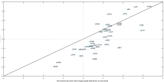
To summarize our sectoral growth rate’s results, the three following …gures contrast each country’s annualized growth rate of aggregate TFP i.e. related to total economy’s outcomes -with its annualized growth rate of sectoral TFP, respectively, on agriculture, industry and ser-vices. These compound annual growth rates represent the TFP growth observed for the period 1996-2009.

(30)

An n u a liz e d g r o w th r a te o f a g g r e g a te to ta l fa c to r p r o d u c tiv ity -4 -3 -2 -1 0 1 2 3 4 A gri cul ture -4 -3 -2 -1 0 1 2 3 4 A US A UT B E L B GR B RA CA N CHN CY P CZE DE U DNK E S P E S T FIN FRA GB R GRC HUN IDN IND IRL ITA JP N K OR LTU LUX LV A ME X MLT NLD P OL P RT ROM RUS S V K S V N S W E TUR TWN US A

Figure 1.2: Annualized Growth Rates of TFP: Agriculture vs. Total Economy

We can note from Figure 2 that, although there has been some considerable dispersion in relative growth rates, only four countries experienced higher annualized growth rates of TFP in agriculture than in the respective economy aggregate, namely Brazil, France, Indonesia and Romania.

Sectoral and total rates have been almost coinciding in Sweden. Cyprus, which had one of the highest annualized growth rate of aggregate TFP, presented the lowest one in agriculture. Bulgaria was the country with the worst TFP growth performance over the period under analysis, responding for the lowest TFP growth rate in total economy and one of the lowest in agriculture.

(31)

31

Annualized growth rate of aggregate total factor productiv ity

-4 -3 -2 -1 0 1 2 3 4 Ind us tr y -4 -3 -2 -1 0 1 2 3 4 AUS AUT BEL BGR BRA CAN CHN CYP CZE DEU DNK ESP EST FIN FRA GBR GRC HUN IDN IND IRL ITA JPN KOR LTU LUX LVA MEX MLT NLD POL PRT ROM RUS SVK SVN SWE TUR TWN USA

Figure 1.3: Annualized Growth Rates of TFP: Industry vs. Total Economy

Figure 3 plots the annualized growth rates of TFP in industry against the annualized growth rates of aggregate TFP. Industry’s relative growth rates were far more concentrated than the agriculture ones but, once again, only a little number of countries had higher annualized growth rates of TFP in industry than in the respective economy aggregate: China, Czech Republic, Estonia, France, Hungary, Ireland, Lithuania, Poland and Slovakia.

The worst performance can again be assigned to Bulgaria and the highest growth rates both in industry and in total economy were observed in China.

(32)

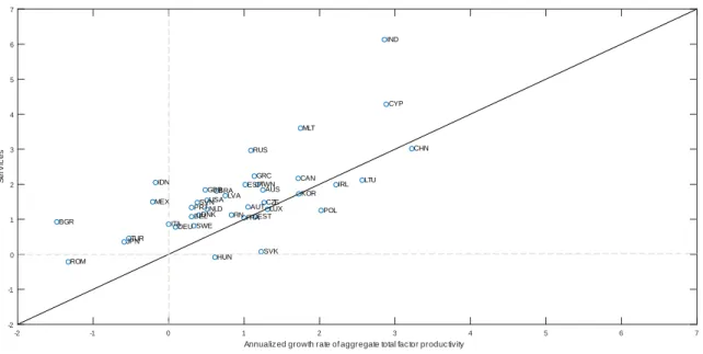
Annualiz ed growth rate of aggregate total fac tor produc tiv ity -2 -1 0 1 2 3 4 5 6 7 S er v ic es -2 -1 0 1 2 3 4 5 6 7 AUS AUT BEL BGR BRA CAN CHN CYP CZE DEU DNK ESP EST FIN FRA GBR GRC HUN IDN IND IRL ITA JPN KOR LTU LUX LVA MEX MLT NLD POL PRT ROM RUS SVK SVN SWE TUR TWN USA

Figure 1.4: Annualized Growth Rates of TFP: Services vs. Total Economy

Lastly, …gure 4 compares the annualized growth rates of TFP in services to the annualized growth rates of aggregate TFP. Contrary to what we observed in the two other sectors, the growth rates of TFP in services were usually higher than the aggregate growth rates for most of the countries.

The exceptions are China, Estonia, Hungary, Ireland, Lithuania, Luxembourg, Poland and Slovakia. Given this, note that all countries presenting annualized growth rates of TFP in industry higher than their aggregate growth rates also presented low relative growth rates in services.

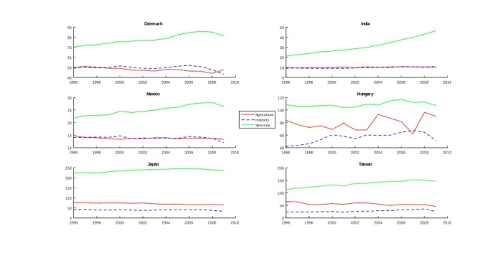
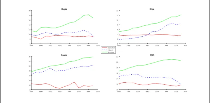
1.4.4 Multi-Country 3-Sector TFP Levels

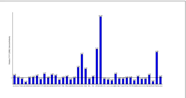
Since showing all 120 TFP level series we obtained from the aggregation in 3 sectors would be fairly counterproductive, in this section we outline some relevant sectoral stylized facts that can be observed from the multi-country 3-sector TFP level series.

First, Figures 5 and 6 show, for the years of 1996 and 2009 respectively and for all countries, the ratio between TFP levels in services and in industry.