Generate disaggregated soil allocation data using a Minimum
Cross Entropy Model
RUI FRAGOSO
Departamento de Gestão de Empresas
Universidade de Évora
Lg. dos Colegiais, 1 – 7004-516 ÉVORA
PORTUGAL
[email protected] http://www.uevora.pt
MARIA DE BELÉM MARTINS
Faculdade de Engenharia dos Recursos Naturais
Universidade do Algarve
Campus de Gambelas, 8005-139 FARO
PORTUGAL
[email protected] http://www.ualg.pt
MARIA RAQUEL VENTURA LUCAS
Departamento de Gestão de Empresas
Universidade de Évora
Lg. dos Colegiais, 1 – 7004-516 ÉVORA
PORTUGAL
[email protected] http://www.uevora.pt
Abstract: - Montado ecosystem in the Alentejo Region, south of Portugal, has enormous agro-ecological and
economics heterogeneities. A definition of homogeneous sub-units among this heterogeneous ecosystem was made, but for them is disposal only partial statistical information about soil allocation agro-forestry activities. The paper proposal is to recover the unknown soil allocation at each homogeneous sub-unit, disaggregating a complete data set for the Montado ecosystem area using incomplete information at sub-units level. The methodological framework is based on a Generalized Maximum Entropy approach, which is developed in thee steps concerning the specification of a r order Markov process, the estimates of aggregate transition probabilities and the disaggregation data to recover the unknown soil allocation at each homogeneous sub-units. The results quality is evaluated using the predicted absolute deviation (PAD) and the “Disagegation Information Gain” (DIG) and shows very acceptable estimation errors.
Key-Words: Montado ecosystem, Cross Entropy, Maximum Entropy, incomplete information, Alentejo.
1. Introduction
Montado ecosystem, integrated in Mediterranean
ecosystems, cover about 1 million hectares in the Alentejo Region, south of Portugal. Oak forests and the savanna-like landscapes, in which Quercus ilex
spp. rotundifolia and Quercus suber are a dominant
part of the agro forestry system, produce fodder for livestock, as well as cork and firewood. It has been extensively used by man in agro-forestry-extensive grazing systems. This use has prevented severe impacts on the ecosystem, even with strong ecological restrictions, such as severe droughts in a summer that is very long.
The Montado ecosystem area in the Alentejo Region (MEA) is far from being homogeneous. There are enormous and varied heterogeneities, namely in what
concerns agro-ecological aspects, that determine the specialization profile of economic activities, particularly the agro-forestry activities.
The determination of homogeneous sub-units is of particular interest. Both international obligations as well as European legislation ask for the assessment of agricultural practices regarding their effects on the environment and on natural resources and ecosystems sustainability. Several models and tools can be used to analyze natural resources use and to simulate or predict the natural resources’ near future consequences of changing land use and farming practices. The main obstacle to use models or modeling tools for environmental impact assessment in agriculture from the regional to continental scale or vice-versa is the difficulty to match agricultural activities with the environmental circumstances where
they are taking place [1; 2] and particularly, detailed data availability. It is necessary to generate and disaggregate relevant data that will allow a much better analysis of socio-economic indicators and will permit their consideration for planning and policy application. Major economic models approaches, as CAPRI [3; 4], SEAMLESS [5], SENSOR [6; 7], EURURALIS [8], INSEA [9], GENEDEC [10] or LUMOCAP [11] deal with linking agricultural production models with economic and environmental aggregate data for estimating relationships, whit consequent aggregation problems.
The proposal of this paper
is to demonstrate the adherence of the minimum crossed entropy model as a process conducting to dynamic spatial information generation and disaggregation. With this model, it will be possible to use the disposable information to generate data disaggregated to homogeneous sub-units (HSU) that can be used on the estimation of these territories’ soil occupation.The paper includes also a reference to the homogenous territorial MEA sub-units, a brief review of the disaggregation data problem, the methodological framework, the results and finally the conclusions.
2. Homogeneous territorial units
The Évora University’s Unit of Macroecology and Conservation studied the representative dominant patterns in the MEA, for all Alentejo parishes, based on:
- Climatic averages; maximum temperature in August; minimum temperature in January; Winter precipitation; Summer precipitation; inland or not; altitude.
- Dominant agro-forestry use - agriculture, forestry or not cultivated.
- Average farm size.
- Type and density of Montado: Quercus ilex spp.
rotundifolia, with low, high and very high
density; Quercus suber, with low, high and very high density; mixed with low, high and very high density; Pinus pinea with low density;
- Livestock: head/ha and proportion of farms with sheep, swine, beef cattle and goats.
A hierarchical multivariate analysis and non-linear methods were used. The results allowed the identification of six homogeneous agro-forestry macro-units in MEA. These macro-units are linked with the diversity and regional specificities of available resources and how they are used and valued by resident populations (Table A1 in Appendix).
The macro-unit A is characteristic from Alentejo inner zones with low precipitation. These zones have generally small forest areas, the Quercus ilex spp.
rotundifolia being the dominant species. Agro-forestry
farms are big – the most part of the area is concentrated in farms over 500 ha. Their economic activity is mainly animal production, particularly cattle and Alentejo swine, in na extensive way. This production pattern determines soil occupation, predominating spontaneous pastures.
Macro-unit B is also present in Alentejo inner zones with low precipitation. Although it also has a low forestry potential, in general, there are some high-density Quercus ilex spp. rotundifolia spots. Agro-forestry farms are medium or small – a significant parto f the área is concentrated in farms between 200 ha and 500 ha. Their main economic activity is cattle production. The soil occupation reflects this, the objective being to produce cattle food – the rotations are usually
long term forages-pastures rotations,
under trees or not.
The macro-unit C occurs in littoral zones with good precipitation level according to regional pattern.
Quercus suber and Quercus ilex spp. Rotundifolia are
present with high densities. Agro-forestry farms are smaller, the area being mainly occupied by farms with less then 200 ha. Vineyards to produce wines with Name of Origin or Quality Wines PSR and the animal production – cattle, sheep and Alentejo swines – are among the main activities.
Macro-unit D occurs on the higher inner zones of Alentejo, with good precipitation level according regional pattern. In the agro-forestry pattern the low-density Quercus ilex spp. Rotundifolia dominates. Farms are medium to big and animal production, mainly catlle and Alentejo swine, are the main activities. As in B, the rotations are usually long term forages-pastures rotations, under trees or not.
The macro-unit E is characteristic from inner zones that are already close to littoral, the frontier zones, with good precipitation level according to regional pattern. There are important high-density Quercus
suber spots. Farms are usually small and their
economic activity is mainly cattle. Food for cattle comes from the farm and is mainly composed of durum wheat straw and stubbles, and spontaneous or improved pastures.
Finally, macro-unit F is associated to Alentejo inner zones with low precipitation levels. Frequently high-density spots of Quercus ilex spp. rotundifolia or
Quercus suber can be observed. Farms are small to
medium. Animal production, mainly cattle, is the main economic activity. Food for cattle comes mainly from the farm – spontaneous and improved pastures, straw and stubbles from cereals. The rotation system
is cereals-long term pastures (spontaneous or improved).
The six identified macro-units were then crossed with environmental protection areas of NATURA 2000 and National Protected Areas.
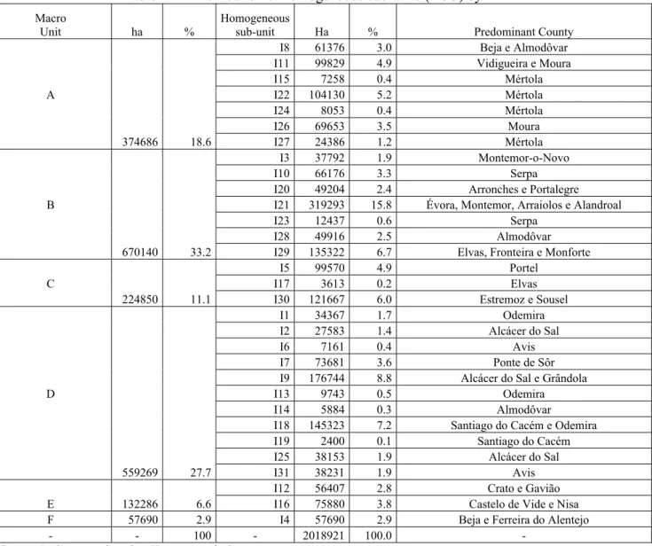
This proceeding allowed the establishment of 31 homogeneous sub-units (HSU), which are a function of their interest for natural values conservation (Table A2 in Appendix).
The pertinent HSU only represents the potential use of resources and not his effective use – this is the result of technical, economical and institutional factors. In her work,
Klimešová
[12] states exactly that when more than one type of data is involved this is sometimes referred to as the ‘intersection’ question since it is needed to find the intersection of data sets. Then, the patterns question allows environmental and social scientists and planners to describe and compare the distribution of phenomena and to understand the processes, which account for their distribution. Therefore, to study the MEA it is necessary to determine the soil allocation for the year 2004, which is the base year for accessing economics. From the Agricultural Census [13] it is possible to recover the soil allocation in each HSU, crossing the available data at county level, but only for years 1989 and 1999. For the remaining years, there is no information at HSU level.The model proposed will allow estimating unknown soil allocation data for the MEA, at HSU disaggregated level in a consistent way. At MEA aggregate level, the soil allocation can be obtained for the series years 1989 to 2004 from 1989 and 1999 Agricultural Census [13], Structural Agricultural Enterprises Surveys of 2003 and 2005 [14] and Annual Agricultural Statistics from 1999 to 2005 [15]. This complete information and the incomplete information known at HSU level for the years 1989 and 1999 can then be used within a maximum entropy framework to estimate the disaggregated unknown data for remaining years until 2004.
The maximum entropy method is a flexible and powerful tool for density approximation. According to Shamilov [16] there is empirical evidence that demonstrates the efficiency of this method. For this reason the MaxEnt distributions are much convenient if data is not well distributed.
3. The disaggregation data problem
Disaggregation data problems are present in many fields like climate science, geography, business or economy [17]. The first valid approaches to go from aggregate data to disaggregate data came from the political science in the beginning of the Twentieth
Century [18]. In economics, the linkage between aggregate models for all economy and disaggregated sectoral models has been a widely recognised problem [19].
According with Howitt and Reynaud [20], valid data disaggregation method is interesting and needed in agricultural production economics empirical studies, for three main reasons. Firstly, because the availability of data and the difficulty of obtaining adequate micro data. The second reason for disaggregation is that consistency among the explanatory variables requires that most microeconomic models are estimated at the level of the least disaggregated variable and, finally, because of the necessity to combine agricultural production models and biophysical process models. As well, You and Wood [21] defend data disaggregation using a cross-entropy approach to generate plausible data and disaggregated estimates of the distribution of crop production on a pixel basis.
One approach to disaggregate data can be to consider some individual behavioural rules to specify aggregate data. Another approach is to infer from aggregate data the most micro behaviour consistent with the observed outcomes. This last one will be adopted in this paper and it will be presented to proceed.
Consider that soil allocation at MEA aggregate level is given by Sk(t), where k=1,...,K corresponds to observed agro-forestry activities and t=1,...T corresponds to the year in which they occur. Then the probability of producing k activity in year t is:
r ,... 1 = t , k , ) t ( kSk ) t ( k S = ) t ( k Y
(1)
The MEA is composed by i=1,…I HSU and the annual probability of each agro-forestry activities occur at this disaggregate level is:
r ,... 1 = t , k , ) t ( k i k s ) t ( i k s = ) t ( i k Y
(2)
The information disaggregated at HSU level in what concerns soil occupation by each agro-forestry activity si
k(t) is available only for the first r periods (r
< T). The data availability assumption is that there is
a complete data set at aggregate level, but only partial information at disaggregated level. In our case there is only disposable information by county from the Agricultural Census of 1989 and 1999.
The challenge is to combine complete information at MEA aggregate level for t=1,…,T with partial information at disaggregated HSU level for t=1,…,r and recover the soil allocations si
k(t) for the periods
t=r+1,...,T. The objective is to obtain a soil allocation
for each HSU consistent with the aggregate data. The estimation of ski must guarantee that soil allocation for each activity at MEA level is equal to the sum of this activity area in all HSU, obeying the following restriction: T ,..., 1 + r = t , k , I i = i ) t ( i k s = ) t ( k S
(3)
This disaggregation data problem presents more parameters to estimate than available moment conditions because K-1>T-r. This problem cannot be solved by the classical methods like least chi-square, maximum likelihood and Bayesian methods. The Shannon [22] entropy methods can be used to obtain a unique optimal solution. They are more and more used in several sciences [23].
In agricultural economics Miller and Platinga [24] applied the ME to estimate land use shares and predicting its impact on soil erosion in three Iowa counties from a multi-county scale. They also showed that the ME approach encompasses the logistic regression as a particular case.
To separate harvested area and yield for irrigated crops from rainfall crops in counties of Texas and California States (USA) Ximing et al. [25] used the principle of ME combined with incomplete data, empirical knowledge and priori information. For a sample of California State (USA) data, that includes six districts in the Central Valley and eight crops, Howitt and Reynaud [20] developed a dynamic data consistent way to estimate agricultural land use choices at a disaggregated level, using more aggregate data. This is done in two steps. First it is specified a ME dynamic model of land allocation at aggregate level. Second, the outcomes are disaggregated from the ME model results using the Minimum Cross Entropy [26]. This method differs from [24] and [25] mainly because the process of soil occupation choice is endogenous.
The cross entropy method can be applied to solving difficult combinatorial optimization problems. The basic mechanism involves an iterative procedure of two phases [27]:
1. draw random data samples from the currently specified distribution.
2. identify those samples which are, in some way, “closest” to the rare event of interest and update the parameters of the currently specified distribution to
make these samples more representative in the next iteration
4. The methodological framework
The methodological framework, based on Howitt et Reynaud [20], consists on a dynamic process of allocating soil inside each HSU of the MEA. It is assumed that the soil allocation follows a finite r-order Markov process, which is a probabilistic model appropriated for time series when the state variable depends only on the previous state values. According to Kijima [28], a sequence of r observations of soil allocation can be characterized by a 1st order Markov process. In this case, any activity choice process, among k possibles activities for the HSU is defined as a 1st order Markov process in the space {1,...Kr}. This means that Kr states of decision are considered, corresponding to Kr possible strategies, indexed by j {1,…J} with J=Kr. The probability associated to each state j in the HSU i and year t is given by qki(t). qki(t) and corresponds to the product of probabilities yki(t) to the sequence of states
j. The soil allocation in a given periodt
{
1,..,T}
only depends on the r previous periods.Assuming a 2nd order Markov process the probability of producing j in t-1 and j’ in t is yi
j(t-1). yij’(t). Let
Ti
jj’(t) be the (Kr×Kr) Markov transition matrix associated to soil allocation at HSU disaggregate level in the period t. This gives the probability of passing from any state j {1,…Kr} to any state j’ {1,…Kr} in the period t+1. Then the probability of being in state
j’ is: {1,...,J}and t {r,...,T-1} 'j , ) t ( J 1 = j i ' jj T ). t ( i j q = ) 1 + t ( i 'j q
(4)
And the probability of producing the k activity in the period t+1 is: ) t ( J 1 = j i ' jj T ). t ( i j q ) k ( 'j = ) 1 + t ( i k y
(5)
As the information available at HSU level only corresponds to the first r observations, the following proceeding has to be taken: 1. Estimate the dynamic soil allocation at MEA aggregate level with a r order Markov process; 2. Specify an aggregate soil allocation using a Generalized Maximum Entropy (GME) model to estimate the aggregate transition probabilities matrix; and 3. Calculate for a given year how disaggregated estimation differs from aggregate and are compatible with the same year aggregate data
using a Minimum Cross Entropy Model and the aggregate transition probabilities before estimates. The problem of recovering transition probabilities can be expressed by the following GME formulation:
)) t ( n 'j e log( ). t ( n 'j e 1 -T r = t N 1 = n J 1 = j' -) m ' jj T log( . m ' jj T M 1 = m J 1 = 'j J 1 = j -= e) H(T, e , T Max
(6)
subject to: t , j' , N 1 = n ) t ( n 'j e . n v + m ' jj T . m w ). t ( j Q M 1 = m J 1 = j = ) 1 + t ( 'j Q(7) j 1 = m ' jj T . m w M 1 = m J 1 = 'j
(8) [ ]0,1 j, j' Tjj' and 1 = m ' jj T M 1 = m
(9)
[ ]
0,1 j', t n j' e and 1 = ) t ( n 'j e N 1 = n(10) where w={w1,…,wM} and v={v1,…,vN} with M 2 and N 2 are the support sets of transition probabilities
{Tjj’1,…,Tjj’M} and of error term {ej’1,…,ej’N}, respectively.
In this optimization problem the objective is to maximize the entropy of probabilities distribution Tjj’m and of error term ej’n under the constraints (7) to (10). According constraint (7), the probability of producing
j’ activity in t+1 year must equal the product of the
probability of producing j activity in t year by the respective transition probabilities and the error term. It is a data consistence constraint, which establishes for each year the soil allocation at MEA aggregate level. The remaining constraints assure the proprieties of probabilities.
After this, it is still needed to estimate for each year the probabilities transition matrix at HSU disaggregated level, solving a problem of minimization of generalized crossed entropy (GCE), and using those estimated transition probabilities to finally obtain soil allocation for each HSU. The problem of GCE can be formulated as:
)) t ( kn e log( ). t ( kn e T 1 + r = t N 1 = n K 1 = k + ) ' jj T / i ' jj T log( . i jj T J 1 = 'j J 1 = j I 1 = i = e) , i H(T e , i T Min (11) subject to: k ) t ( kn e . n N 1 = n + i ' jj T ). t ( i j q ) k ( 'j J 1 = j I 1 = i i s = ) 1 + t ( k S (12)
[ ]
0,1 j ' i ' jj T and 1 = i ' jj T J 1 = 'j i, (13)[ ]
0,1 j'et kn e and 1 = ) t ( kn e N 1 = n (t) (14)where { 1,..., N} with N 2 is the support vector associated to error probabilities {ek1t,…,ekNt}, si is the area of each i HSU, Tˆjj'is the aggregate transition probabilities matrix obtained before with the GME model and Ti
jj’is the to be estimate transition probabilities matrix at HSU disaggregated level. This model minimizes the cross entropy of the transition probabilities distribution with noise (11), under the constraints (12) to (14). The compatibility data constraint (12) assures that for each year the total soil allocated to activity k in all HSU disaggregated level must be the same allocated to this activity k at the MEA aggregate level (Sk). The last two constraints concern the proprieties of the probability distribution. The HSU soil allocation is available only for the first
r years, which can be directly computed for t=r. For
the remaining years t=r+1,…,T the transition probabilities matrix Ti
jj’ and the error term ekn are estimated year to year. Then this information is used to recover the soil allocation at HSU disaggregated level.
5. Results
The GME model formulated in equations (6) to (10) was solved as a non-liner optimization problem with the General Algebraic Modelling System (GAMS). Before solving the model it was necessary to establish the support values for the parameters and errors. The natural bounds of w={w1,…wM} and v={v1,…vN} are zero and one. According to [11], 3 support points for vector w were chosen – w={0, 0.5, 1}. For error support
v the N is also 3 and the bounds were determined using
the 3 rule [20].
To estimate the transition probabilities matrix at aggregate level the GME model was applied to MEA data years of 1989 and 1999 to 2004.
The model includes 14 agro-forestry activities, which covers the most important soil allocation activities observed at MEA. These activities include soft wheat production, durum wheat production, maize, rice, melon, tomato, sunflower, olive groves, vineyards, fruits, pastures, forages, fallow and shrubs and forest.
Based on the Agricultural Census of 1989 and 1999, Surveys on Agricultural Structures from 2003 to 2005 and Economic Accounts of Agriculture from 2000 to 2005 the first order Markov processes were established, which translate the probability of each agro-forestry activity to happen (and therefore, the MEA soil occupation) for years 1989, 1999, 2000, 2001, 2002, 2003 and 2004. Therefore, to estimate the probabilities distribution in each year, we used K=14 activities and
T=7 years, which gives 196 possible Markov states
(K×K) for each year.
For each year a transition probabilities matrix is obtained.
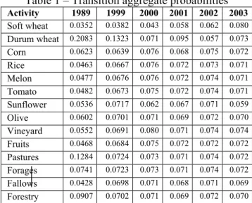
Table 1 presents the annual transition probabilities for the years of 1989 and 1999 to 2003 by activity. In the transition probabilities matrix columns represents the forestry activities at t year and lines the agro-forestry activities at t-1 year. Each element of Table 1 is the yearly probability of any agro-forestry activity to be produced at year t after any other agro-forestry activity has been produced in the previous year t-1. For example, the probability of produce soft wheat in 1999 after any agro-forestry activity produced in 1989 is 3.52%.
To evaluate the coherence of the estimated transition probabilities, the predicted results were compared with the observed values from years 1989 and 1999 to 2004 and calculated the prescription absolute deviation (PAD) by soil allocation activity:
100 × k y k y -k y = k PAD
Table 1 – Transition aggregate probabilities
Activity 1989 1999 2000 2001 2002 2003 Soft wheat 0.0352 0.0382 0.043 0.058 0.062 0.080 Durum wheat 0.2083 0.1323 0.071 0.095 0.057 0.073 Corn 0.0623 0.0639 0.076 0.068 0.075 0.072 Rice 0.0463 0.0667 0.076 0.072 0.073 0.071 Melon 0.0477 0.0676 0.076 0.072 0.074 0.071 Tomato 0.0482 0.0673 0.075 0.072 0.074 0.071 Sunflower 0.0536 0.0717 0.062 0.067 0.071 0.059 Olive 0.0602 0.0701 0.071 0.069 0.072 0.070 Vineyard 0.0552 0.0691 0.080 0.071 0.074 0.074 Fruits 0.0468 0.0684 0.075 0.072 0.072 0.072 Pastures 0.1284 0.0724 0.073 0.071 0.074 0.072 Forages 0.0741 0.0723 0.073 0.071 0.074 0.072 Fallows 0.0428 0.0698 0.071 0.068 0.071 0.069 Forestry 0.0907 0.0702 0.071 0.069 0.072 0.070
Source: GME model results
The PAD results presented in the Table 2 shows that the model allows a good prescription of the soil allocation at MEA aggregate level.
The biggest PAD values, which reflects the major differences between predicted and observed soil allocation activities, occurs at 1999 year, namely on durum wheat (27.8%), corn (38%), melon (27.7%) and vineyards (46.2%). The PAD values are also highs for tomato in 2000 and 2001 and for melon in 2000. The remains PAD values are below 15%, which is the value considered by Hazell et al. [29] as the reasonable calibration threshold. The good quality of the GME model results can be confirmed through the weighted PAD. In this case the PAD is obtained for all the MEA and presents very low values, which varies between 2.3% at 1999 year and less 1% for the remains years.
Table 2 – Predicted Absolute Deviation
Activity 1999 2000 2001 2002 2003 2004 Soft wheat 0.5 4.0 15.4 16.9 26.7 18.4 Durum wheat 27.8 3.7 0.2 0.6 0.6 0.1 Corn 38.0 8.0 0.6 8.9 4.6 0.9 Rice 10.7 9.2 3.4 5.2 1.5 1.4 Melon 27.7 21.6 9.2 0.8 0.8 0.4 Tomato 14.8 30.6 21.3 13.1 15.8 3.8 Sunflower 1.9 1.1 4.8 2.8 1.0 9.2 Olive 0.5 0.2 0.2 0.1 0.2 0.0 Vineyard 46.2 3.5 11.2 2.8 2.5 4.7 Fruits 14.9 7.7 4.5 4.5 36.6 23.2 Pastures 0.2 0.0 0.0 0.0 0.0 0.0 Forages 1.2 0.2 0.1 0.0 0.0 0.0 Fallows 0.0 0.0 0.0 0.0 0.0 0.0 Forestry 1.1 0.0 0.1 0.1 0.5 0.0 Source: Statistical data and predicted results with GME estimators
After estimated the dynamic process of soil allocation at aggregate MEA level, it is necessary to use this information as prior in the GCE model to estimates the HSU disaggregated transition probabilities. Then the disaggregated soil allocation is recovered year by year using the equation (15). These results should be compared with the reality, which can only be done to the year 1999, as for the other years there are no disaggregated results. It must be stated that the estimations obtained with this model were close to the reality in 1999.
To evaluate the results quality we also used the weighted predicted absolute deviation (WPAD), calculated as follows, for each activity and HSU:
K 1 k i k DAPP i DAPP e i k y i k y -i k y i k y i k DAPP = = =
and at MEA aggregate level:
i k DAPP I 1 i . S i s DAPP = =
Table 3 shows that in general the results obtained to HSU disaggregated level are good. The WPAD values by activity were relatively low. Values above 15%, only occur for permanent pastures and fallow and, even thought, only for 7 of the 31 HSU. Nevertheless, these differences do not compromise the validity of disaggregation process. In reality, many of the permanent pastures are integrated in very long rotations and subject to very low number of heads per hectare and the fallows are frequently used as spontaneous pastures. So, the errors can be accommodated in current practices that can not be reflected in the disposable statistical information.
Table 3 – Weighted Predicted Absolute Deviation by HSU disaggregated level
HSU WPAD HSU WPAD HSU WPAD HSU WPAD
I1 35.7 I9 14.7 I17 23.0 I25 58.6
I2 23.5 I10 35.7 I18 16.6 I26 60.8
I3 41.4 I11 25.4 I19 24.5 I27 15.4
I4 23.4 I12 26.3 I20 21.1 I28 17.0
I5 56.5 I13 25.7 I21 21.4 I29 14.8
I6 28.2 I14 55.1 I22 43.9 I30 27.3
I7 25.6 I15 54.0 I23 34.1 I31 25.6
I8 25.7 I16 24.8 I24 66.9 Total 25.7
Source: Statistical data and predicted results with GCE estimations
The WPAD per HSU present values above 25% in about half of the cases. However the total WPAD, which considers the agro-forestry activity and HSU weights for all MEA, is 27.3%, which is an acceptable value.
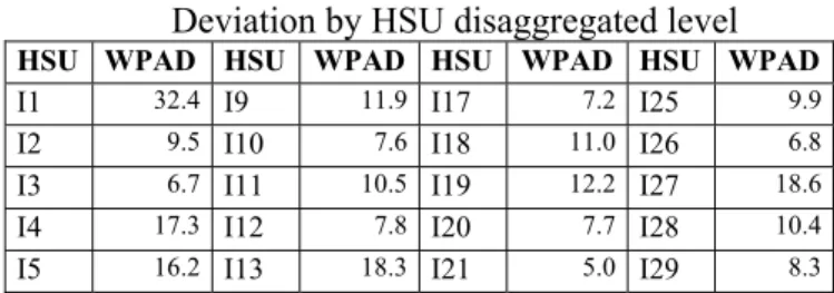
Analysing the WPAD for each HSU, considering pastures and fallows together as the same agro-forestry activity, the total WPAD of 27.3% obtained before falls to 10.5% (see Table 4). Furthermore the biggest PAD value is now 32.4% and only in six HSU this indicator is above 15%, which is the reasonable calibration threshold. Unlike the PAD values presented in Table 3, the PAD values of Table 4 are perfectly accepted as estimation errors and confirm the good method’s adherence to disaggregate soil allocation data.
Table 4 – Adjusted Weighted Predicted Absolute Deviation by HSU disaggregated level
HSU WPAD HSU WPAD HSU WPAD HSU WPAD
I1 32.4 I9 11.9 I17 7.2 I25 9.9
I2 9.5 I10 7.6 I18 11.0 I26 6.8
I3 6.7 I11 10.5 I19 12.2 I27 18.6
I4 17.3 I12 7.8 I20 7.7 I28 10.4
I5 16.2 I13 18.3 I21 5.0 I29 8.3
I6 9.8 I14 12.5 I22 14.6 I30 8.8
I7 14.8 I15 16.8 I23 8.3 I31 11.6
I8 14.6 I16 5.1 I24 19.2 Total 10.5 Source: Statistical data and predicted results with GCE estimations
Another way of analysing the interest of this method to the given problem is to measure the information gain from the disaggregation process. For that it is necessary an indicator that measures the quantity of information that is changed due to aggregation process. Howitt et Reynaud [20] construct an indicator, the “Disagegation Information Gain” (DIG), based on the cross entropy between the observed values of soil allocation at aggregate (yk) and disaggregated (yik) level and on the crossed entropy between the soil allocation estimated by the disaggregation model (yˆik) and those observed at HSU disaggregated level (yi
k). The crossed entropy values are calculated as:
K 1 = k yik k y ln . k y I 1 = i = CE and K 1 = k yik i k yˆ ln . i k yˆ I 1 = i = Eˆ C
Then the DIG is given by:
CE Eˆ C 1 = DIG
CE is the entropy measure of the distance between the observed soil allocation at MEA aggregate and HSU disaggregated level, while CÊ is the entropy measure of how far the HSU disaggregated estimates are from the observed values. This way DIG measures the proportion of heterogeneity at HSU level that is covered by the disaggregation process used.
In a perfect disaggregation, DIG is equal to 1. In this case, the disaggregation process recovers 100% of information heterogeneity because yˆik.=yik. If there is no heterogeneity in the information, it is the case where
yk=yik, the DIG is 0. The DIG varies between 0 and 1 and increases as the disaggregated estimates are closer to the observed data values.
Our model obtained a DIG of 0.43, which means the disaggregation recovers 43% of the information heterogeneity at the 31 HSU level, considering the 14 agro-forestry activities for soil allocation. These results are very satisfactory, especially when compared to the DIG values between 56 to 69% obtained by Howitt et Reynaud [20] in an information disaggregation process for only six districts of California State (USA) and eight crops activities.
6. Conclusions
This work estimates the unknown soil allocation data at homogeneous sub-units disaggregated level for the
Montado ecosystem in the Alentejo Region. The
disaggregation process is based on a Generalized Maximum Entropy methodological framework that use complete information at aggregate level of Montado ecosystem area and incomplete information at disaggregated level of theirs homogeneous sub-units. The method is developed in three steps. In the first it is established an r order Markov process, which represents the dynamic soil allocation at the Montado ecosystem aggregated level. The second step concerns the estimates of transition probabilities within a Generalized Maximum Entropy model of aggregate soil allocation. The last step consists in disaggregating the aggregate data using a Generalized Cross Entropy model and in recovering the unknown soil allocation at each homogeneous sub-units.
The achieved results show very acceptable estimation errors. It can be concluded that the methodological framework proposed is able to disaggregate the values that exist at Montado ecosystem area level to each of its homogeneous sub-units level, allowing the representation of soil allocation each year.
Economic sustainability is an important part of the sustainability issue and the economic analysis is surely the framework of the structural policy analysis that impacts the territory and of the future scenarios’ study, technical and economic management models and evaluation of determinant factors.
It is of fundamental interest to have a tool that allows the information generation for homogeneous sub-units, giving the basis to study socio-economic parameters and the impact of agricultural policy scenarios on the natural resources exploitation.
References:
[1] Liu, Y., Yu, Z., Chen, J., Zhang, F., Doluschitz, R., and Axmacher, J. C. Changes of soil organic carbon in an intensively cultivated agricultural region: A denitrification-decomposition (DNDC) modelling approach, Science of the Total Environment, 372, 203– 214, 2006.
[2] Mulligan, D. T. Regional modelling of nitrous oxide emissions from fertilised agricultural soils 25 within Europe, PhD thesis, Bangor, University of Wales, 2006. [3] Britz, W., Pérez, I., Zimmermann, A. Heckelei, T. Definition of the CAPRI Core Modeling System and Interfaces with other Components of SEAMLESS-IF,
Report no.: 26, January 2007
[4] Britz, W. EU-wide spatial down-scaling of results of regional economic models to analyze environmental impacts, 107th EAAE Seminar "Modelling of
Agricultural and Rural Development Policies". Sevilla,
Spain, January 29th -February 1st, 2008.
[5] Elbersen, B., Kempen, M., van Diepen, K., Andersen, E., Hazeu, G. and Verhoog, D. Protocols for spatial allocation of farm types. SEAMLESS report no.
19, 2006
[6] Jansson, T., Bakker, M., Hasler, B., Helming, J., Kaae, B., Neye, S., Ortiz, R., Sick Nielsen, T., Verhoog, D. and Verkerk H. Description of the modelling chain.
SENSOR Deliverable 2.2.1. In: Helming K , Wiggering
H, (eds.): SENSOR Report Series 2006/5,
http://zalf.de/home_ipsensor/products/sensor_report_ser ies.htm, ZALF, Germany
[7] Kristensen, P., Frederiksen, P., Briquel, V. and Parachini, M.L. SENSOR indicator framework, and methods for aggregation/dis-aggregation – a guideline.
In: Helming K , Wiggering H, (eds.): SENSOR Report
Series 2006/5,
http://zalf.de/home_ipsensor/products/sensor_report_ser ies.htm, ZALF, Germany.
[8] Verburg, P.H., Schulp, C.J.E., Witte, N. and Veldkamp A. Downscaling of land use change scenarios to assess the dynamics of European landscapes. Agriculture, Ecosystems & Environment: Volume 114, Issue 1, 39-56.
[9] Adler et.al. INSEA (Integrated Sink Enhancement Assessment), Final Report, IASSA, 2007.
[10] Chakir R. Spatial downscaling of Agricultural Land Use Data: An econometric approach using cross-entropy method. Toulouse: Inra. 2007
[11] Van Delden, H. and Luja P. Integration of multi-scale dynamic spatial models for land use change analysis and assessment of land degration and socio-eonomic processes. In: Proceeding from the conference
on Soil protection strategy - needs and approaches for policy support, Polawy, Poland 9-11th March 2006.
[12] Klimešová, D. Study on Geo-information Modelling, WSEAS Transactions on Systems. 5, 2006, 5 pp. 1108-1113.
[13] INE - Instituto Nacional de Estatística (1989 e 1999) Recenseamento Geral Agrícola - RGA.
[14] INE - Instituto Nacional de Estatística (2003 e 2005) Inquérito à Estrutura das Explorações Agrícolas
- IEEA.
[15] INE - Instituto Nacional de Estatística (1999 a 2005) Estatísticas Agrícolas - EAA.
[16] Shamilov A. A Development of Entropy Optimization Methods, WSEAS Transactions on
Mathematics, 5, 2006, 5, 568-575.
[17]Von Storch, Zorita, H. and Cubash, U. Downscaling of global climate change estimates to regional scales: An application to Iberian rainfall in wintertime, Journal of Climate. 6, 1993, pp. 1161-1171.
[18] King, G. A Solution to the Ecological Inference
Princeton, Princeton University Press, 1997.
[19] Barker, T. and Pesaran, M. Disaggregation in Econometric Modeling – An Introduction, In
Disaggregation in Econometric Modeling, London, T.
Barker and M. Pesaran editors, 1990.
[20]
Howitt, R & Reynaud, A. Spatial Disaggregation of Agricultural Production Data using Maximum Entropy, European Review of Agriculture Economics Vol. 30,No. 3, 2003 pp.359-387.[21] You, L. and Stanley W. Assesing the Spatial Distribution of Crop Production Using a Cross-Entropy Method, EPTD Discussion Paper No. 126, Environment and Production Technology Division International Food Policy Research Institute, Washington, D.C., U.S.A. 2004.
[22] Shannon, C. A Mathematical Theory of Communication (1 and 2), Bell Systems Tech, 27, 379-423 and 623-656, 1948.
[23] Dionisio, A., Meneses, R. and Mendes, D. A Entropia como Medida de Informação na Modelação Económica, In Temas em Métodos Quantitativos, edited by Elizabeth Reis and Manuela Magalhães Hill, Edições Sílabo, 2003.
[24] Miller, D. and Plantinga, A. Modeling Land Use Decisions with Aggregate Data. American Journal of
Agricultural Economics, Vol. 81, No. 1, 1999, pp.
180-194.
[25] Ximing, C., De Fraiture, C., and Hejazi, M. Retrieval of irrigated and rainfed crop data using a general maximum entropy approach. Irrigation
Science, 25, 2007, pp. 325-338.
[26] Golan, A., Judge, G. & Miller D. Maximum
Entropy Econometrics: Robust Estimation with Limited Data, New York, John Wiley Editions, 1996.
[27] Wu, Y. and Fyfe, C. The On-line Cross Entropy
Method for Unsupervised Data Exploration, WSEAS
Transactions on Mathematics, 2008.
[28] Kijima, M. Markov processes for stochastic
modelling, Chapman & Hall London, 1997.
[29] Hazell, P.B.R. & Norton, R.D. Mathematical
Programming for Economic Analysis in Agriculture,
Appendix
Table A1- Alentejo representative Montado Agro-Forestry Production Systems (MAPS)
MAPS
Soil occupation Livestock activity
Forest characteristics Climatic factors Agricultural economy aspects A Pastures under trees Cattle and swine Weak forest. Predominance of Quercus ilex spp.
rotundifolia
Inner zones, with low level of precipitation Big farms: 1366 ha UAS and 6 AWU B
Gras and grazings activities, under trees or
not
Cattle Quercus ilex spp. rotundifolia with high
density
Inner zones, with low level of precipitation
Medium and small farms: 377 ha UAS and 2,42 AWU
C
Olive oil and vineyards systems and gras and
grazings activities
Cattle and
sheep rotundifolia and Quercus Quercus ilex spp. suber with high density
Littoral zones with good level of precipitation Small farms: 177 ha UAS and 6,43 AWU D
Gras and grazings activities, under trees or
not
Cattle and
swine rotundifolia with low density Quercus ilex spp. with good level of High inner zones precipitation
Medium to big farms: 798 ha UAS and 4,21
AWU E
Cereals and pastures, under trees or not
Cattle Quercus suber with high
density
Inner zones near littoral with good
level of precipitation in
Winter
Small farms: 107 ha UAS and 1,15 AWU
F Cereals and pastures, under trees or not Cattle rotundifolia and Quercus Quercus ilex spp. suber with high density
Inner zones with low level of precipitation
Small to medium farms: 448 ha UAS
and 3,05 AWU Source: k-means analysis, done by the Évora University’s Unit of Macroecology and Conservation
Table A2 – Distribution of homogeneous sub-units (HSU) by MEA
Macro
Unit ha %
Homogeneous
sub-unit Ha % Predominant County
I8 61376 3.0 Beja e Almodôvar
I11 99829 4.9 Vidigueira e Moura
I15 7258 0.4 Mértola A I22 104130 5.2 Mértola I24 8053 0.4 Mértola I26 69653 3.5 Moura 374686 18.6 I27 24386 1.2 Mértola I3 37792 1.9 Montemor-o-Novo I10 66176 3.3 Serpa
I20 49204 2.4 Arronches e Portalegre
B I21 319293 15.8 Évora, Montemor, Arraiolos e Alandroal
I23 12437 0.6 Serpa
I28 49916 2.5 Almodôvar
670140 33.2 I29 135322 6.7 Elvas, Fronteira e Monforte
I5 99570 4.9 Portel
C I17 3613 0.2 Elvas
224850 11.1 I30 121667 6.0 Estremoz e Sousel
I1 34367 1.7 Odemira
I2 27583 1.4 Alcácer do Sal
I6 7161 0.4 Avis
I7 73681 3.6 Ponte de Sôr
I9 176744 8.8 Alcácer do Sal e Grândola
D I13 9743 0.5 Odemira
I14 5884 0.3 Almodôvar
I18 145323 7.2 Santiago do Cacém e Odemira
I19 2400 0.1 Santiago do Cacém
I25 38153 1.9 Alcácer do Sal
559269 27.7 I31 38231 1.9 Avis
I12 56407 2.8 Crato e Gavião
E 132286 6.6 I16 75880 3.8 Castelo de Vide e Nisa
F 57690 2.9 I4 57690 2.9 Beja e Ferreira do Alentejo
- - 100 - 2018921 100.0 -