Testing consumption optimality using aggregate data

(1)

Ensaios Econômicos

Escola de

Pós-Graduação

em Economia

da Fundação

Getulio Vargas

N◦ 756 ISSN 0104-8910

Testing Consumption Optimality using

Ag-gregate Data*

Fábio Augusto Reis Gomes, João Victor Issler

(2)

Os artigos publicados são de inteira responsabilidade de seus autores. As

opiniões neles emitidas não exprimem, necessariamente, o ponto de vista da

Fundação Getulio Vargas.

ESCOLA DE PÓS-GRADUAÇÃO EM ECONOMIA Diretor Geral: Rubens Penha Cysne

Vice-Diretor: Aloisio Araujo

Diretor de Ensino: Carlos Eugênio da Costa Diretor de Pesquisa: Humberto Moreira

Vice-Diretores de Graduação: André Arruda Villela & Luis Henrique Bertolino Braido

Augusto Reis Gomes, Fábio

Testing Consumption Optimality using Aggregate Data*/ Fábio Augusto Reis Gomes, João Victor Issler – Rio de Janeiro : FGV,EPGE, 2014

25p. - (Ensaios Econômicos; 756)

Inclui bibliografia.

(3)

Testing Consumption Optimality using Aggregate Data

Fábio Augusto Reis Gomes Department of Economics

University of São Paulo – Ribeirão Preto [email protected]

João Victor Isslery

Graduate School of Economics – EPGE Getulio Vargas Foundation

[email protected] August, 2014.

Keywords: Consumption Optimality, Intertemporal Substitution, Risk Aversion, Aggregate Return, Habit, Rule-of-Thumb Behavior, Representative-Consumer Model.

JEL Classi…cation: C22; D91; E21.

Abstract

This paper tests the optimality of consumption decisions at the aggregate level taking into

account popular deviations from the canonical constant-relative-risk-aversion (CRRA) utility

function model – rule of thumb and habit. First, based on the critique in Carroll (2001) and

Weber (2002) of the linearization and testing strategies using euler equations for consumption, we

provide extensive empirical evidence of their inappropriateness – a drawback for standard

rule-of-thumb tests. Second, we propose a novel approach to test for consumption optimality in this

context: nonlinear estimation coupled with return aggregation, where rule-of-thumb behavior

and habit are special cases of an all encompassing model. We estimated 48 euler equations

using GMM. At the 5% level, we only rejected optimality twice out of 48 times. Moreover,

out of 24 regressions, we found the rule-of-thumb parameter to be statistically signi…cant only

We are especially grateful to two Anonymous Referees, Caio Almeida, Marco Bonomo, Luis Braido, Carlos

E. Costa, Russell Davidson, Pedro C. Ferreira, Karolina Goraus, Fredj Jawadi (Editor), Anwar Khyat, Naércio A.

Menezes Filho, for their comments and suggestions on earlier versions of this paper. We also bene…ted from comments

given by the participants of ISCEF conferences in Paris, 2014, where this paper was presented. The usual disclaimer

applies. Fabio Augusto Reis Gomes and João Victor Issler gratefully acknowledge support given by CNPq-Brazil.

Issler also acknowledges the support given by CAPES, Pronex, FAPERJ, and INCT. We gratefully acknowledge

research assistance given by Rafael Burjack, Marcia Waleria Machado and Marcia Marcos.

y_{Corresponding Author. Address: Graduate School of Economics – EPGE, Getulio Vargas Foundation, Praia de}

(4)

twice. Hence, lack of optimality in consumption decisions represent the exception, not the rule.

Finally, we found the habit parameter to be statistically signi…cant on four occasions out of 24.

1 Introduction

For the U.S. economy, there has been a large early literature using time-series data rejecting optimizing behavior in consumption which generated some relevant puzzles; see Hall (1978), Flavin (1981), Hansen and Singleton (1982, 1983, 1984), Mehra and Prescott (1985), Mark (1985), Camp-bell and Deaton (1989), and Weil (1989). Most of these studies employed the constant-relative-risk-aversion (CRRA) utility function with exponential discounting of future utility in de…ning welfare. These rejections have led to two di¤erent strands of the consumption literature. The …rst inves-tigated whether changing preferences could accommodate optimizing behavior; see Abel (1990) and Campbell and Cochrane (1999) for research on habit, and Epstein and Zin (1989, 1991) for research on non-expected utility. The second strand introduced explicit forms of non-optimizing behavior for consumption decisions. On that regard, the most in‡uential study is that of Camp-bell and Mankiw (1989, 1990), who extended the basic optimizing model incorporating what they have labelled rule-of-thumb behavior: there are two types of consumers, the …rst type consumes according to optimizing behavior but the second consumes only his/her current income1. In this setup, changes in aggregate consumption respond to expected changes in aggregate income, and the response is a function of the importance of rule-of-thumb consumers.

In the context above, rejecting optimizing behavior using aggregate data (time series) is an im-portant setback in macroeconomics, where it is commonly assumed an optimizing representative-consumer framework with a CRRA utility function. Moreover, this rejection has far-reaching implications: it raises the issue of whether or not we can postulate optimizing behavior in Macro-economics – if one cannot defend optimizing behavior at the aggregate level, one can question whether it is applicable at all.

This paper has two original contributions to the literature on consumption optimality at the aggregate level. Our setup tests for optimality having as a basis the standard CRRA framework for the representative consumer, where the generalized method of moment (GMM) is used in estimation and testing. We employ an encompassing model that simultaneously allows for the existence of rule-of-thumb behavior and habit in preferences, which are tested as exclusion restrictions. Our limited

(5)

focus on these two departures stem for historical reasons: most of the literature in macroeconomics have employed the CRRA utility function, while the main deviations from optimality are the presence of rule-of-thumb consumers in Campbell and Mankiw (1989, 1990), and the extension in Weber (2002), dealing jointly with rule of thumb and habit in preferences2. Next, we detail our main contributions.

First, at least since Carroll (2001), its is well-known that ignoring higher-order terms in log-linearization of euler equations yields inconsistent estimates of their respective parameters, inval-idating hypothesis testing. This happens because past observed values do not constitute valid instruments, but these are exactly the instruments the previous literature has used. As shown below, this critique applies directly to linear or log-linear rule-of-thumb tests. In a direct test of the omission of higher-order terms in log-linearized models, we con…rm empirically their misspeci-…cation. Results of auxiliary misspeci…cation tests also concur with the latter.

Second, we circumvent the problem of lack of instruments in log-linearized regressions by using a nonlinear setup for estimation and testing. Our approach has two main ingredients. The …rst is to exploit the nonlinearity of the euler equation of the optimizing agent, where, under rule of thumb, her/his consumption is a linear combination of consumption and income (Weber, 2002)3_.

The second is to aggregate returns in the euler equation for the optimizing agent. This is possible because the latter allows linear aggregation of gross returns, although it is a nonlinear function of consumption and preference parameters.

Aggregating returns has several bene…ts: (i) from a theoretical point-of-view, we know that only pervasive variation of returns a¤ects intertemporal substitution in consumption4. Due to the law-of-large numbers, aggregation preserves the pervasive variation of returns, throwing away

2_{Note that, by itself, habit does not constitute a deviation from optimality.}

3_{For the habit speci…cation, it is also a function of a linear combination of lagged consumption and income.}

4_{The quote in Mulligan (2002) summarizes well why aggregating returns is a good strategy:}

“If we were interested, say, in the willingness of consumers to substitute food for other goods, then we

should look at the correlation between food expenditure and a food price index. This correlation would

have little relation with the correlation between food expenditure and the price of carrots, unless there

were a perfect correlation between the price of carrots and the price of all other foods. There may be

theories of food demand implying that the price of carrots is always in the same proportion to other

food prices, but if in fact there were something moving the price of carrots apart from the prices of other

foods, then a price index for all foods is needed. By analogy, my paper compares consumption growth

(6)

idiosyncratic variation. This allows a representative-consumer interpretation of utility parameters, where aggregate consumption is matched with aggregate returns – not with a handful of individual returns; (ii) estimating euler equations for several assets requires knowledge ofparticipation – what assets are used to transfer wealth across time in every period; see Vissing-Jørgensen (2002), and Attanasio, Banks, and Tanner (2002)5. Although this may be a problem for panel-data studies, participation at the aggregate level is readily available from …nancial markets, wealth surveys, and national accounts; (iii) standard GMM estimation employing a large number of returns is usually infeasible because the number of time periods is small vis-a-vis the number of assets. Return aggregation preserves the pervasive portion of return variation, allowing feasible estimation. On the other hand, if one focuses on a subset of returns in empirical tests, as it is commonly done in the literature, asset-return information is thrown away – which is sub-optimal from an econometric point of view.

Our empirical implementation for testing optimality in consumption decisions, rule-of-thumb behavior, and habit in preferences, requires the use of an aggregate return measure for the economy as a whole – what Mulligan (2002) labelled the return to aggregate capital. Here, we employ prox-ies of the return to aggregate capital in two di¤erent frequencprox-ies: the annual measures computed by Mulligan (2002) and Mulligan and Threinen (2010), and the quarterly measures computed by Mulligan and Threinen (2010). When these measures are used in estimation and testing, we pro-vide unequivocal epro-vidence that the log-linearization of the representative-consumer euler equation is problematic. Beyond linearization, and within the CRRA model context, we provide strong evidence against rule-of-thumb behavior for U.S. consumers and against habits in consumer pref-erences. Our results are in sharp contrast to those in Campbell and Mankiw regarding rule of thumb and to those in Weber regarding habit. Indeed, we show that we can appropriately repre-sent preferences for the U.S. reprerepre-sentative consumer using a CRRA utility function with an annual discount rate of 0:95 and a relative-risk-aversion coe¢cient roughly between 1 and 2, depending on whether we employ consumption of nondurables or consumption of nondurables and services in estimation. Regarding the main objective of this paper – test consumption optimality at the aggregate level – we found very little evidence of rejection of optimality in consumption decisions when over-identifying-restriction tests are employed, although, on occasion, there were rejections.

5_{Vissing-Jørgensen (2002) and Gross and Souleles (2002) have split households in groups. Large estimates of the}

intertemporal elasticities of substitution in consumption - around 0.8 - when stock return was used for stockholders

(7)

Once proper models and econometric techniques are applied to aggregate consumption, income, and aggregate return data, there is no reason to challenge optimizing behavior in consumption, as was the case with previous rule-of-thumb tests. We also show that augmented models for preferences such as consumption with habit formation are unnecessary to characterize intertemporal substitution having the canonical CRRA model as a starting point. Of course, that does not mean that a broader model could not also …t the data6. All in all, our evidence reduces the fear that optimizing behavior is the exception, not the rule.

The paper proceeds as follows. Section 2 presents the consumption models, the linear and the nonlinear consumer euler equation, as well as the asset returns aggregation. Section 3 presents the econometric methodology. Section 4 presents the empirical results, and Section 5 concludes.

2 Consumption Models

2.1 The Standard Approach in Macroeconomics – CRRA Utility with

Aggre-gate Data

The standard approach in macroeconomics consists of a single-good economy of identical con-sumers, whose utility functions are of the CRRA type:

u(Ct) =

C_t1 1

1 (1)

where Ct is consumption in periodt, and is the constant relative risk-aversion coe¢cient. Sub-ject to a budget constraint and transversality conditions, consumers choose consumption and asset holdings to maximize the lifetime utility, given byE0P1t=0 tu(Ct), where 2(0;1)is the intertem-poral discount factor, and the mathematical expectation operator Et( ) is formed conditional on information available to the consumer up to periodt. The representative agent can transfer wealth from one period to the next by buying individual assets, indexed by i, i = 1;2; ; N, whose returns are de…ned asRi;t = Pi;t_P_i;t+D₁i;t;wherePi;t and Di;t are respectively their price and dividend. In this setup, the well-known nonlinear euler equation is given by:

Et 1

(

Ct

Ct 1

Ri;t )

= 1; i= 1;2; : : : ; N; (2)

see Hansen and Singleton (1982, 1983, 1984).

(8)

2.2 Testing Consumption Rule of Thumb in a Linear Framework

If one assumes a CRRA utility function, arriving at the euler equation (2), further assuming joint conditional log-Normality and homoskedasticity of Ct

Ct 1; R1;t; R2;t; ; RN;t

0

, the usual time series log-linear representation of consumption growth rate is obtained:

lnCt= + 1

ri;t+ i;t, (3)

where ri;t ln (Ri;t), (

ln +1 2

2 )

, and 2 = V ARh lnCt 1ri;t i

. The error term i;t is unpredictable, since it is an innovation regarding the optimizing agent’s information set. The coe¢cient of the rate of return,1= , is the elasticity of intertemporal substitution (EIS), being the reciprocal of the constant relative risk-aversion coe¢cient, .

The conditions under which equation (3) is derived are very stringent: i;tj t 1 N 0; 2_i

for all i, with t 1 representing the information set of the optimizing agent. The fact that i;t is conditionally Gaussian and uncorrelated with elements of the conditioning set t 1 implies that

i;t and i;t s,s >0 are independent. Moreover, i;t must be independent of any function of the variables in t 1. In principle, residual-based tests of normality, conditional homoskedasticity, and

serial correlation can be used to ensure that these restrictions apply to _i;t. These will be used below as auxiliary tests in log-linearized euler equations.

Campbell and Mankiw (1989, 1990) proposed rule-of-thumb behavior for consumers at the ag-gregate level. There are two types of consumers: type 1 consumes according to optimizing behavior. Type 2, on the other hand, is restricted to consume her/his current income (y2;t). Income of the

non-optimizing agent holds a …xed proportion ( )to aggregate income as follows, = y2;t

yt , leading

toC2;t =y2;t = yt, where C2;t is agent’s 2 consumption. For the optimizing agent, the literature considers two benchmark cases. The …rst imposes Hall’s (1978) quadratic utility setup, where con-sumption of the optimizing agent follows a martingale process, i.e.,Et( C1;t+1) = 0;whereC1;t is type 1 consumption. A broader benchmark case imposes CRRA utility for the optimizing agent, leading to a log-linear equation for testing H0 : = 0, having aggregate consumption growth as

the regressand:

ln (Ct) = ln (yt) + (1 ) + 1ri;t + (1 ) i;t. (4)

2.3 A Critique of Current Rule-of-Thumb Tests

(9)

“In principle, the theoretical problems with Euler equation estimation stem from ap-proximation error. The standard procedure has been to estimate a log-linearized, or …rst-order approximated, version of the Euler equation. This paper shows, however, that the higher order terms are endogenous with respect to the …rst-order terms (and also with respect to omitted variables), rendering consistent estimation of the log-linearized Euler equation impossible. Unfortunately, the second-order approximation fares only slightly better.”

Along these lines, Araujo and Issler (2011) generalized this result, showing that estimation of approximations that omit higher-order terms do not have standard valid instruments, which consist of lagged values of observables. Their setup exploits the generalized taylor expansion (not an approximation) of the exponential function aroundx;with incrementh, showing that it does not depend onx. Applied to the Asset-Pricing Equation (2), their results allow writing its log-linearized version as follows:

ln (Ct) = ln ( )

+ 1ri;t+E

t 1(zi;t)

+ _i;t; i= 1;2; : : : ; N, (5)

where Et 1(zi;t)

captures the e¤ect of the higher-order terms of the general taylor expansion, withzi;t being the higher-order term in each equation. In generalEt 1(zi;t)will be a function of the variables

in the conditioning set used by the econometrician to compute Et 1( ). Therefore, omission of

Et 1(zi;t)

(or of parts of it) in estimating (5) will generate an omitted-variable bias. This will turn out to be a major problem for versions of (5). It must be stressed that the only reason why this term is present in (5) is because we use a log-linear approximation of (2). Thus, we can circumvent the problem if we do not try to log-linearize it.

2.4 Nonlinear Euler Equation and Return Aggregation

Using a nonlinear instrumental variable estimator – e.g., a generalized method-of-moment (GMM) estimator – we can estimate the following system and test hypotheses of interest:

Et 1fMtRi;tg=Et 1

(

Ct

Ct 1

Ri;t )

= 1; i= 1;2; : : : ; N; (6)

(10)

E¢cient estimation of preference and other parameters in system (6) requires estimating the whole system instead of just a portion of it. This happens for the same reason why single-equation OLS estimation is less e¢cient than SURE estimation in the context of a system of linear regressions. However, system estimation may pose a problem in this context, since, in practice, the number of traded assets(N)in a real economy is large relative to the number of time-series observations (T). For that reason, most of the literature opted to limit the size of N, e.g., N = 2: a risky and a “riskless” asset or, at most, a handful of assets or portfolios with a limited asset coverage. Of course, this solution is sub-optimal at the cost of e¢ciency.

In an interesting paper, Mulligan (2002) shows that an alternative to estimating the system as a whole is cross-sectional aggregation, where we do not throw away useful information contained in Ri;t, i = 1;2; : : : ; N, but rather aggregate returns across i to isolate the common component of asset returns; see also the alternative approach in Araujo and Issler (2011). Support for cross-sectional aggregation in this context is based on the idea that idiosyncratic risk, uncorrelated with

Mt, must be irrelevant for intertemporal substitution, and cross-sectional aggregation naturally eliminates it. If N is su¢ciently large, return aggregation will deliver the common component of returns associated with intertemporal substitution, allowing matching aggregate consumption with an aggregate return.

In what follows we present a stylized version of Mulligan’s approach. Consider the sequence of deterministic weightsf!igNi=1, such thatj!ij<1uniformly onN, with

N X

i=1

!i = 1or lim

N!1

N X

i=1

!i=

1, depending on whether we allow or not the existence of an in…nite number of assets.

Cross-sectional aggregation of (5) implies:

ln (Ct) = 1 ln ( ) +1rt+ 1

Et 1(zt) + t, (7)

where rt = N P i=1

!iri;t is the logarithm of the return to the geometric average of aggregate capital,

zt = N P i=1

!izi;t, and t = N P i=1

!i i;t. Notice that we can specialize !i = 1=N to use equal weights in aggregation. Despite aggregating returns, Mulligan omits the term 1Et 1(zt) in estimating (7),

potentially leading to an omitted-variable bias.

(11)

sample moments. Despite that, since for allithe orthogonality conditions hold, we can form a cross-sectional averageeh( ; wt) = _N1

N P i=1

h( ; wi;t), and estimate by GMM fromE eh( ; wt) = 0. Under

a set of standard assumptions, Driscoll and Kraay prove consistency and asymptotic normality for the GMM estimates of . That happens whether N is …xed orN ! 1.

It is important to stress that, although the approach in Mulligan may be inappropriate due to the use of a linear consumption model, it is a clever way of preserving information on all returns that would otherwise be lost ifN is large relative toT. Using aggregate returns, we show next how to construct an encompassing consumption model that allows simultaneously for the existence of rule-of-thumb behavior and habit in preferences. These two departures from the standard CRRA model can then be tested as exclusion restrictions for the parameters of the encompassing model.

As in Weber (2002), the key issue is to note that the optimizing agent – type 1 – obeys the euler equation. Since we want to allow for habit and rule of thumb, we start with preferences with habit for the optimizing agent:

u(C1;t; C1;t 1) =

(C1;t C1;t 1)1 1

1 , 6= 1: (8)

The optimizing agent euler equation is:

Et 1

8 < :

(C1;t 1 C1;t 2) (C1;t C1;t 1) [ +Ri;t]

+ (C1;t+1 C1;t) Ri;t

9 =

;= 0; all i. (9) Recall that aggregate consumption must be the sum of the consumption of the two types. Thus,

C1;t=Ct yt. Substituting the latter into (9):

Et 1

8 > > > < > > > :

[(Ct 1 yt 1) (Ct 2 yt 2)]

[(Ct yt) (Ct 1 yt 1)] [ +Ri;t]

+ [(Ct+1 yt+1) (Ct yt)] Ri;t 9 > > > = > > > ;

= 0; all i. (10)

Notice that (10) is a general model that encompasses rule of thumb and habit, under CRRA. It has three special cases: habit alone ( = 0), rule of thumb alone ( = 0), and neither habit nor rule of thumb ( = = 0), which is the case of CRRA utility. Equation (10) only depends on observables, although C y is highly persistent, which can be dealt with transformations using ratios: Ct=Ct 1, Ct=yt, etc. Although (10) is nonlinear on consumption, it allows (linear) aggregation and averaging of Ri;t across i, leading to GMM estimation as long as instruments are not indexed byi. Start with:

Et 1

u0₍_C

t yt; Ct 1 yt 1)

u0₍_C

t 1 yt 1; Ct 2 yt 2)

(12)

Center, post-multiply by instruments Xt 1, and use the law of iterated expectations:

E u

0₍_C

t yt; Ct 1 yt 1)

u0₍_C

t 1 yt 1; Ct 2 yt 2)

Ri;t 1 Xt 1 = 0; all i. (12)

From Driscoll and Kraay, cross-sectionally aggregate (12), using weightswi,0 wi 1,PNi=1wi= 1, with Rt=

N P i=1

wiRi;t. Denote the terms in brackets of (12) by h( ; wi;t). Then, their aggregate

version is:

e

h( ) = N X

i=1

wih( ; wi;t) =

u0₍_C

t yt; Ct 1 yt 1)

u0₍_C

t 1 yt 1; Ct 2 yt 2)

Rt 1 Xt 1;

where it becomes clear that we can estimate = ( ; ; ; )0 by GMM using:

Eneh( )o=E u

0₍_C

t yt; Ct 1 yt 1)

u0₍_C

t 1 yt 1; Ct 2 yt 2)

Rt 1 Xt 1 = 0: (13)

The euler equation behind the moment restrictions (13) is interpretable and can be viewed as that of the optimizing agent who holds a portfolioRt=

N P i=1

!iRi;t in every period7. A natural way to construct weights (!i or!i;t) is to look at participation of di¤erent assets on the portfolio of aggregate wealth in every period. This is motivated by the fact that euler equations of the form in (10) only hold as an equality in t if asset iis being used to transfer wealth from t 1 to t. This is a crucial issue when testing for optimality, since the euler equation must hold under the null hypothesis.

Participation is discussed by Vissing-Jørgensen (2002), and Attanasio, Banks, and Tanner (2002) in a panel-data context. There, the main problem is that we do not possess the information on speci…c assets used to smooth out consumption across time for every individual. However, for the representative consumer, one has the information on the composition of aggregate wealth. Mulligan referred to the composite returnRtin the following terms: “the interest rate in aggregate theory is not the promised yield on a Treasury Bill or Bond, but should be measured as the expected return on a representative piece of capital.” In our view, this is the return that should be used to recover interpretable preference parameters for the representative consumer. For that reason, optimality tests here will be conducted using the encompassing model (13) in the form of a J-test (Sargan test) as discussed in Hansen (1982).

7_{For simplicity of notation we use weights that do not depend on time}_t_,_!_{i. However, there is no problem with}

(13)

3 Econometric Methodology

3.1 Data

The critical series used in this study is the aggregate real interest rate represented by Rt in (13) above, which is used to uncover (or identify) the structural preference parameters of the representative consumer. Rt here is measured in di¤erent forms. The …rst measure is the capital rental rate after income and property taxes in the U.S., as computed by Mulligan (2002), and its updated version measured as the annual and quarterly estimates of the net marginal product of capital in the U.S., as computed by Mulligan and Threinen (2010)8_{. These two measures are}

identical, in a context where aggregate capital exists and its marginal product is net of depreciation9. The …rst proxy is available in annual frequency from 1947 to 1997, whereas the second is available from 1930 to 2009 on an annual frequency. We use only the annual post-war data from 1950 onwards and the quarterly data from 1950:1 onwards.

The rest of the data used here were extracted from the U.S. National Income and Product Account (NIPA) and from the U.S. Census Bureau. From NIPA, we extracted annual data for real disposable personal income, nominal consumption of nondurables and its price index, and nominal services consumption and its price index. We used two measures of consumption in this paper, following almost all of the consumption literature: real consumption of nondurables and real consumption of nondurables and services. Unfortunately, there is no de‡ator for nondurables plus services. Thus, we aggregated nondurables and services using Irving Fisher’s ideal price index – an equally weighted geometric average of the Laspeyres and Paasche price indices. Intuitively, by employing Fisher’s method, we allow rebalancing the weights of the parts on the sum of the components. Simply summing up the de‡ated parts implies keeping these weights …xed throughout the whole post-war sample, which is obviously inappropriate. To obtain per capita series we used

8_{We thank Casey Mulligan for providing data on both papers to us.}

9_{To show that the marginal return to aggregate capital is identical to} _R

t =

PN

i=1!iRi;t, up to addition of a constant term, notice that, if we give weights according to participation of the value of total capital in the previous

period, !i =

Vi;t 1 PN

i=1Vi;t 1, recalling that the marginal return of each asset iis Ri;t 1 =

Yi;t

Vi;t 1, where Yi;t is the

current income accrued from asseti, including dividends and capital gains, and thatPN

i=1!i= 1, then:

Rt 1 = N

X

i=1

!i(Ri;t 1) = N

X

i=1

Vi;t 1 PN

i=1Vi;t 1 Yi;t

Vi;t 1

=

PN i=1Yi;t PN

i=1Vi;t 1 ;

the last term being exactly the measure constructed by Mulligan (2002) and Mulligan and Threinen (2010) – total

accrued aggregate income divided by last period’s total capital value. Thus, for our estimated regressions, we added

(14)

population data from the US Census Bureau.

3.2 Estimating and Testing Log-Linear Models

Our approach for testing the appropriateness of log-linear models has a direct test for omitted higher-order terms and an auxiliary approach that employs diagnostic tests verifying whether or not the stringent conditions under which an exact log-linear model holds are ful…lled.

The direct test employed here is a modi…ed Ramsey’s RESET test, designed to work within an instrumental-variable (IV) context. The standard version of Ramsey’s RESET test is based on low order polynomials of the predicted value of the dependent variable, e.g., y^2, y^3 and y^4. The signi…cance of any of these terms indicates misspeci…cation. Under simultaneity, Pagan and Hall (1983) and Pesaran and Taylor (1999) extended the application of RESET tests. Here, we perform their RESET tests considering the signi…cance of three groups os higher-order terms: y^2_; _y_^2 _and

^

y3;y^2,y^3 andy^4.

The auxiliary testing procedure is designed to apply the following diagnostic tests: homoskedas-ticity, no serial-correlation, and normality tests, all designed to work within and IV context. The homoskedasticity tests applied here are: Pagan and Hall’s (1983) test, White/KoenkerT R2 _test,

and Breusch-Pagan/Godfrey/Cook-Weisberg test. No serial correlation of the error term is in-vestigated by means of the Cumby and Huizinga (1992) test. Finally, we employ Shapiro-Wilk, Jarque-Bera, and Shapiro-Francia Normality tests.

3.3 Estimating and Testing Nonlinear Models under Rule-of-Thumb and Habit

Since consumption and income are known to have roots of the autoregressive polynomial equal (or nearly equal to) to unity, we transform euler equations to achieve stationarity. In the context of rule-of-thumb tests, Weber (2002) discusses this issue at some length, dividing euler equations by speci…c powers ofyt to generate non-integrated terms. These powers depend on preferences. Here, we opted for a slightly di¤erent route. For the preferences in (1) or (8), dividing euler equations by Ct 1 generates terms that have the following formats: gross growth rates of consumption or

income, income-to-consumption or consumption-to-income ratios, or products of them.

We list below the four euler equations in untransformed and transformed formats, highlighting the transformations performed in order to achieve stationarity.

(15)

equation (10). Collecting terms and multiplying (10) by _C1

t 1 gives the following transformed model:

Et 1

8 > > > > > < > > > > > :

[Rt+ ] h

Ct

Ct 1

yt

Ct 1 1

yt 1 Ct 1

i

Rt 2 h_C

t+1 Ct 1

yt+1 Ct 1

Ct

Ct 1

yt

Ct 1 i

1 yt 1 Ct 1

Ct 1 Ct 2

1 _C

t 1 yt 2

1 9 > > > > > = > > > > > ;

= 0: (14)

2. Optimizing agent with external habit and no rule-of-thumb. The untransformed model is given in equation (10), with = 0. Collecting terms and multiplying the resulting equation by _C1

t 1 gives the following transformed model:

Et 1

8 > < > :

[Rt+ ] _CC_tt₁ Rt 2 C_Ct_t+1₁ _CC_tt₁

1 Ct 2 Ct 1

9 > = >

;= 0: (15)

3. Optimizing agent with CRRA utility, rule-of-thumb, and no habit. The untransformed model is given in equation (10), with = 0. Dividing the numerator and denominator of Ct yt

Ct 1 yt 1 by Ct 1, gives,

Et 1

8 < :

Ct

Ct 1

yt

Ct 1 1 yt 1

Ct 1 !

Rt 1

9 =

;= 0 (16)

4. Optimizing agent with CRRA utility – no rule-of-thumb and no habit. The model is already in stationary form:

Et 1

"

Ct

Ct 1

Rt 1

#

= 0: (17)

The transformed models (i.e., equations (14)-(17)) are estimated by GMM using the continu-ously updating method of Hansen, Heaton and Yaron (1996), which has shown superior properties vis-a-vis alternative methods in empirical simulations. As instruments, we employ only lags of observables in each equation being considered10_.

4 Empirical Results

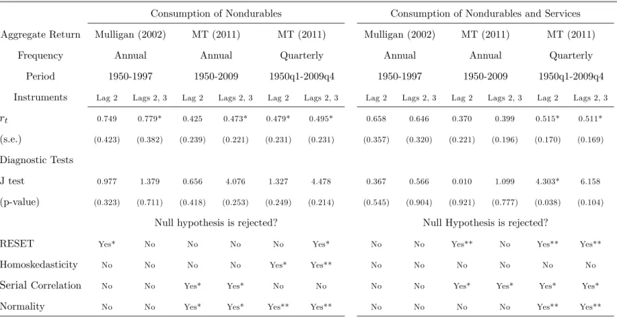
First of all, we present the results for linear models. Table 1 reports the estimation of log-linear models of the form in (3) for consumption of nondurables and consumption of nondurables and services. First, notice that the model is not rejected by the J-test on any occasion, at the 5% level. However, in additional misspeci…cation tests (direct test of omission of higher-order terms

(16)

and auxiliary tests) it is rejected on every occasion by at least one test, with three exceptions – annual frequency, 1950-1997, with nondurables and lags 2 and 3 as instruments, with nondurables and nondurables and services, and lags 2 and 3 as instruments. Overall, most rejections occur in Normality and Serial-correlation tests, followed by rejections in RESET tests.

In Table 2 we test the log-linear model for rule-of-thumb under the same two alternative mea-sures of consumption. The direct RESET tests for omitted higher-order terms rejected the null of their exclusions in 8 out of 12 cases. When we also consider the results of auxiliary tests, with one exception – consumption of nondurables and services, annual frequency from 1950-1997, lags 2 and 3 as instruments – for every regression run, there is a rejection on at least one of the speci…cation tests discussed above. Given the poor performance of the log-linearized model so far, our next step is to focus on nonlinear estimation results.

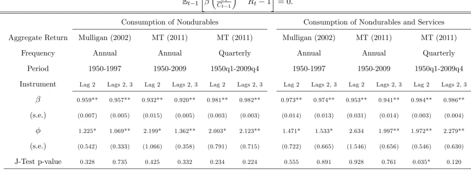
Table 3 presents GMM estimation of the encompassing model allowing for habit and rule of thumb – equation (14). We …rst look at annual data collected by Mulligan (2002) and Mulligan and Threinen (2010). Regardless of whether one uses consumption of nondurables or of nondurables and services, there are no rejections using Hansen’s (1982) J-test of over-identifying restrictions. Moreover, in no occasion we rejected either = 0 or = 0 using robust t-ratios. Evidence with quarterly data is not so overwhelming: we still …nd no rejections of optimality usingJ-tests. However, when we employ nondurables and services, there is evidence that the habit parameter is statistically signi…cant at the 5% level, with _b' 0:95 on two occasions11. Changing the measure of consumption to nondurables take us back to the same results with annual data. We still …nd no rejection on J-tests and neither nor are statistically signi…cant anywhere. Taking the whole evidence into account points toward simplifying the encompassing model in both dimensions, one at a time (equation (15) or (16)).

We consider next restricting the encompassing model with = 0, resulting in a pure habit model – equation (15). The results are displayed in Table 4. For annual data, we …nd no rejections for over-identifying-restriction tests (optimality), as well as no rejection of = 0 with robust t-ratios at5%. For quarterly data, we rejected = 0on two occasions when we employ nondurables and services12_{. In one of them, we also rejected optimality using the} _J_{-test. Still, when we used}

consumption of nondurables alone, we neither found statistically signi…cant nor we rejected

1 1_{It is interesting no note that, on these two rejections of} _{= 0}_{, the estimates of} _{jumped from the interval}_[1_;₃_:_5]

to7:1and15:2, respectively. Empirically, the continuously updating estimator of Hansen, Heaton and Yaron (1996) displays fat tails, which may be the case here on these occasions.

(17)

optimality when J-test are employed.

Table 5 presents GMM estimation of rule of thumb models for the constrained agent. J-tests never reject the over-identifying restrictions implied by the model. Moreover, in all but two cases, we did no …nd the rule-of-thumb parameter to be statistically signi…cant at the 5% level. Signi…cant rule-of-thumb parameter occurred for nondurable consumption with annual data (1950-2009), instruments lags 2 and 3, and quarterly data with instruments lagged twice. It is worth noting that, on these two instances, estimated values of are close to 0:2, well below the0:5values found by Campbell and Mankiw. Still on Table 5, the relative-risk-aversion coe¢cient and the discount factor are signi…cant almost everywhere with plausible values: between 1 and 2 for the former and around0:95 (annually) for the latter. So, our next step is to examine the CRRA case.

Finally, Table 6 presents GMM estimation of the basic CRRA model. J-tests only reject the restrictions implied by over-identifying restrictions once: lag 2 instruments with quarterly frequency. Still, the relative-risk-aversion coe¢cient and the discount factor are signi…cant almost everywhere with plausible values: is not statistically di¤erent from 1 or2, depending on the consumption measure used, and is statistically equal to0:95 (annually) mostly everywhere.

All in all, we estimated 48 euler equations using GMM, with encouraging results vis-a-vis the optimality of consumption decisions – the title of this paper. If we take the level of signi…cance to be 5%, we only rejected optimality twice out of 48 times. Regarding the issue of whether we can still rely on the canonical CRRA model, our opinion that the evidence here supports its use with a few caveats: after all, out of 24 regressions testing the signi…cance of habit or rule of thumb, we found the rule-of-thumb parameter to be statistically signi…cant at the 5% level only twice, and the habit parameter to be statistically signi…cant on four occasions. So, the overall evidence supports optimality under CRRA utility whenever an aggregate return is used13.

5 Conclusions

This paper has the following contributions to the literature on consumption optimality. First, following up on the critique in Carroll (2001), we show empirically that the omission of higher-order terms in the log-linear approximation of euler equations yields inconsistent estimates of the structural parameters when lagged observables are used as instruments. This critique extends to

1 3_{This raises the question of whether we would reach a similar conclusion if we have had a large sample of time}

periods and returns with feasible GMM estimation, i.e., if we perform system estimation with a large number of

(18)

standard rule-of-thumb tests using a log-linearized model. Second, we show that the nonlinear estimation of a system of N Asset-Pricing Equations can be done e¢ciently even if the number of asset returns (N) is high vis-a-vis the number of time-series observations (T), where system estimation is infeasible. We argue that e¢ciency can be restored by aggregating returns into a single measure that fully captures intertemporal substitution. Indeed, there is no reason why return aggregation cannot be performed in the nonlinear setting of the Asset-Pricing Equation, since the latter allows for linear aggregation of individual returns. Third, aggregation of the nonlinear euler equation forms the basis of a novel optimality test and tests of deviations from the canonical CRRA model of consumption in the presence of rule-of-thumb and habit behavior.

One of our main empirical results was to be able to back out plausible and precise preference-parameter estimates for the representative consumer, where the corresponding euler-equation re-strictions were not rejected by over-identifying-restriction tests. All in all, our estimates show that we can describe reasonably well the U.S. representative consumer with an annual discount rate of 0:95 and a relative-risk-aversion coe¢cient roughly between1 and 2, depending on whether we employ consumption of nondurables or consumption of nondurables and services in estimation.

References

[1] Abel, A., (1990). “Asset prices under habit formation and catching up with the Joneses”, American Economic Review Papers and Proceedings,80, 38-42.

[2] Araujo, F. and Issler, J.V. (2011). “A stochastic discount factor approach to asset pricing using panel data asymptotics.” Working Paper: Graduate School of Economics, Getulio Vargas Foundation. Ensaios Econômicos da EPGE # 717.

[3] Attanasio, O.P., Banks, J. and Tanner, S. (2002). “Asset holding and consumption volatility”, Journal of Political Economy, 110(4), 771–792.

[4] Breusch, T.S. and Pagan, A.R. . (1979). “A simple test for heteroskedasticity and random coe¢cient variation”,Econometrica, 47, 1287–1294.

[5] Campbell, J.Y. and Cochrane, J. (1999). “Force of habit: a consumption-based explanation of aggregate stock market behavior”,Journal of Political Economy, 107(2), 205-251.

(19)

[7] Campbell, J.Y., Mankiw, N.G. (1989). “Consumption, income and interest rates: reinterpret-ing the time series evidence.” In: Blanchard, O.J., Fischer, S. (Eds.),NBER Macroeconomics Annual. MIT Press, Cambridge, MA, 185-214.

[8] Campbell, J.Y., Mankiw, N.G. (1990). “Permanent income, current income, and consumption.” Journal of Business and Economic Statistics, 8, 265-280.

[9] Carroll, C.D. (2001). “Death to the log-linearized consumption euler equation! (And very poor health to the second-order approximation)”,The B.E. Journal of Macroeconomics, 1(1), 1-38. [10] Cumby, R.E. and Huizinga, J. (1992). “Testing the autocorrelation structure of disturbances in ordinary least squares and instrumental variables regressions”,Econometrica, 60(1), 185-195. [11] Driscoll, J.C. and Kraay, A.C. (1998). “Consistent covariance matrix estimation with spatially

dependent panel data”,The Review of Economics and Statistics, 80(4), 549-560.

[12] Epstein, L.G. and Zin, S.E. (1989). “Substitution, risk aversion, and the temporal behavior of consumption and asset returns: a theoretical framework”,Econometrica, 57, 937-968.

[13] Epstein, L.G., Zin, S.E. (1991). “Substitution, risk aversion and the temporal behavior of consumption and asset returns: an empirical analysis”, Journal of Political Economy, 99, 263-286.

[14] Flavin, M.A., (1981). “The adjustments of consumption to changing expectations about future income”,Journal of Political Economy, 89, 974-1009.

[15] Hall, R.E. (1978). “Stochastic implications of the life cycle-permanent income hypothesis: theory and evidence”,Journal of Political Economy, 86, 971-87.

[16] Hall, R.E. (1988). "Intertemporal substitution in consumption”,Journal of Political Economy, 96, pp. 339–357.

[17] Hansen, L.P., Heaton, J. and Yaron, A. (1996). “Finite-sample properties of some alternative GMM estimators”,Journal of Business and Economic Statistics, 14(3), 262–280.

(20)

[19] Hansen, L.P., Singleton, K.J. (1983). “Stochastic consumption, risk aversion, and the temporal behavior of asset returns”, Journal of Political Economy, 91, 249-265.

[20] Hansen, L.P., Singleton, K.J. (1984). Erratum of the article “Generalized instrumental vari-ables estimation of nonlinear rational expectations models”, Econometrica, 52(1), 267-268. [21] Jarque, C.M. and Bera, A.K. (1987). “A test for normality of observations and regression

residuals”,International Statistical Review, 55, 163-172.

[22] Mehra, R. and Prescott, E. (1985). “The equity premium: a puzzle”, Journal of Monetary Economics, 15, 145-161.

[23] Mulligan, C. (2002). “Capital, interest, and aggregate intertemporal substitution”, NBER working paper # 9373.

[24] Mulligan, C. and Threinen, L. (2010). “The marginal products of residential and non-residential capital through 2009”,NBER Working Paper # 15897.

[25] Pagan, A. R. and Hall, D. (1983). “Diagnostic tests as residual analysis”,Econometric Reviews, 2(2), 159–218.

[26] Pesaran, M. H. and Taylor, L. W. (1999). “Diagnostics for IV regressions”,Oxford Bulletin of Economics and Statistics, 61(2): 255–281.

[27] Vissing-Jørgensen, A. (2002). “Limited asset market participation and the elasticity of in-tertemporal substitution”,Journal of Political Economy, 110, 825–853.

[28] Weber, C.E. (2002). “Intertemporal non-separability and “rule of thumb” consumption.” Jour-nal of Monetary Economics, 49, 293-308.

(21)

Table 1 - Instrumental-variable estimation for consumption and capital aggregate return

lnCt= +1rt+errort

Consumption of Nondurables Consumption of Nondurables and Services

Aggregate Return Mulligan (2002) MT (2011) MT (2011) Mulligan (2002) MT (2011) MT (2011)

Frequency Annual Annual Quarterly Annual Annual Quarterly

Period 1950-1997 1950-2009 1950q1-2009q4 1950-1997 1950-2009 1950q1-2009q4

Instruments Lag 2 Lags 2, 3 Lag 2 Lags 2, 3 Lag 2 Lags 2, 3 Lag 2 Lags 2, 3 Lag 2 Lags 2, 3 Lag 2 Lags 2, 3

rt 0.749 0.779* 0.425 0.473* 0.479* 0.495* 0.658 0.646 0.370 0.399 0.515* 0.511*

(s.e.) (0.423) (0.382) (0.239) (0.221) (0.231) (0.231) (0.357) (0.320) (0.221) (0.196) (0.170) (0.169)

Diagnostic Tests

J test 0.977 1.379 0.656 4.076 1.327 4.478 0.367 0.566 0.010 1.099 4.303* 6.158

(p-value) (0.323) (0.711) (0.418) (0.253) (0.249) (0.214) (0.545) (0.904) (0.921) (0.777) (0.038) (0.104)

Null hypothesis is rejected? Null Hypothesis is rejected?

RESET Yes* No No No No Yes* No No Yes** No Yes** Yes**

Homoskedasticity No No No No Yes* Yes** No No No No No No

Serial Correlation No No Yes* Yes* No No No No Yes* Yes* Yes* Yes*

Normality No No Yes* Yes* Yes** Yes** No No No No Yes** Yes**

Note: MT (2010) refers to Mulligan and Threinen (2010). Regression estimated by two-stage least squares using Newey and West’s (1987) procedure for robust S.E.

The instrument lists is composed of lags of the observables in the equation being estimated. ** and * means signi…cant at 1% and 5%, respectively. RESET linearity tests

used here are described in Pagan and Hall (1983) and Pesaran and Taylor (1999). Error serial correlation is investigated by means of the test in Cumby and Huizinga (1992).

The null of Homoskedasticity is investigated by tests in Pagan and Hall (1983), the White-Koenker test, and Breusch-Pagan/Godfrey/Cook-Weisberg test.

Finally, we employ Shapiro-Wilk, Jarque-Bera, and Shapiro-Francia Normality tests.

(22)

Table 2 - Instrumental-variable estimation for consumption and capital aggregate return

ln (Ct) = ln (yt) + (1 ) + 1rt +errort

Sample Period 1950-1997 1950-2009 1950q1-2009q4 1950-1997 1950-2009 1950q1-2009q4

Instruments Lag 2 Lags 2, 3 Lag 2 Lags 2, 3 Lag 2 Lags 2, 3 Lag 2 Lags 2, 3 Lag 2 Lags 2, 3 Lag 2 Lags 2, 3

rt -0.201 -0.040 0.053 0.082 0.759 0.242 0.283 0.246 0.181 0.203 0.803 0.330*

(s.e.) (0.518) (0.519) (0.183) (0.185) (0.565) (0.257) (0.412) (0.404) (0.172) (0.183) (0.708) (0.163)

lnYt 0.943 0.548 0.732 0.584 -0.654 0.600 0.339 0.248 0.378 0.318 -0.719 0.440*

(s.e.) (0.642) (0.406) (0.377) (0.302) (0.948) (0.395) (0.297) (0.222) (0.272) (0.231) (1.353) (0.216)

Diagnostic Tests

J test 0.005 2.720 0.077 1.790 0.189 8.579 0.032 3.473 0.089 4.114 1.230 4.837

(p-value) (0.941) (0.606) (0.781) (0.774) (0.664) (0.073) (0.857) (0.482) (0.766) (0.391) (0.267) (0.304)

Null hypothesis is rejected? Null Hypothesis is rejected?

RESET Yes* Yes* No Yes** No Yes** Yes* Yes* No No Yes* Yes**

Homoskedasticity Yes** Yes* Yes* Yes* Yes** Yes** No No No No Yes** Yes**

Serial Correlation No No No No No Yes* No No Yes** No No No

Normality Yes* No No No Yes** Yes** No No No No Yes** Yes**

Note: See Note in Table 1.

(23)

Table 3 - GMM estimation for consumption, aggregate capital return and income

Et 1 8 > > > > > < > > > > > :

[Rt+ ]

h

Ct Ct 1

yt

Ct 1 1

yt 1

Ct 1

i

Rt 2

h_Ct +1 Ct 1 yt+1 Ct 1 Ct Ct 1 yt Ct 1 i

1 yt 1

Ct 1 Ct 1 Ct 2 1 _Ct 1 yt 2 1 9 > > > > > = > > > > > ; = 0

Instrument Lag 2 Lags 2, 3 Lag 2 Lags 2, 3 Lag 2 Lags 2, 3 Lag 2 Lags 2, 3 Lag 2 Lags 2, 3 Lag 2 Lags 2, 3

0.944** 0.952** 0.946** 0.939** 0.988** 0.992** 0.989** 0.971** 0.964** 0.954** 0.812** 0.776

(s.e.) (0.073) (0.019) (0.018) (0.007) (0.007) (0.009) (0.044) (0.012) (0.044) (0.028) (0.278) (0.707)

1.135 1.207 2.289 1.910** 2.781 3.408 2.376 1.377* 3.217 2.795* 7.096** 15.169

(s.e.) (3.376) (1.547) (1.152) (0.440) (1.559) (1.972) (2.189) (0.587) (2.449) (1.339) (2.635) (10.866)

0.138 0.076 -0.564 -0.432 -0.971 -2.025 0.224 0.075 0.150 0.385 0.018 0.008

(s.e.) (0.325) (0.094) (1.279) (0.324) (1.285) (3.198) (0.161) (0.129) (0.674) (0.714) (0.093) (0.087)

0.460 0.566 -1.059 -1.084 -0.622 -0.702 0.262 0.002 -0.223 -0.658 0.966** 0.949**

(s.e.) (0.487) (0.563) (4.028) (1.900) (0.733) (0.875) (0.420) (0.276) (0.931) (4.317) (0.029) (0.082)

J-Test p-value 0.277 0.667 0.151 0.473 0.565 0.906 0.585 0.861 0.985 0.912 0.714 0.900

Note: MT (2010) refers to Mulligan and Threinen (2010). Models estimated by the continuously updating GMM method of Hansen, Heaton, and Yaron (1996).

The instrument lists is composed of lags of the observables in the equation being estimated. ** and * means signi…cant at 1% and 5%, respectively.

(24)

Table 4 - GMM estimation for consumption and aggregate capital return

Et 1 8 > < > :

[Rt+ ] _CtCt₁

Rt 2 Ct_Ct+1₁ _CtCt₁ 1 Ct_Ct 2₁

9 > = >

;= 0

0.959** 0.958** 0.943** 0.937** 0.982** 0.977** 0.876** 0.938** 1.287 1.041* 0.988 0.895*

(s.e.) (0.006) (0.006) (0.023) (0.018) (0.004) (0.011) (0.153) (0.098) (0.754) (0.294) (1.813) (0.414)

1.258* 1.121* 2.976 2.528 2.084* 0.569 1.437 1.452 2.932* 2.804 2.053** 2.008**

(s.e.) (0.523) (0.436) (1.817) (1.313) (0.927) (2.919) (0.851) (0.727) (1.362) (1.380) (0.187) (0.052)

-1.038 0.099 -1.047 0.053 -0.176 0.870 -0.261 -0.075 -0.707 -0.126 0.778** 0.900**

(s.e.) (12.533) (0.261) (2.717) (0.215) (0.472) (0.839) (0.598) (0.240) (3.083) (0.361) (0.240) (0.025)

J-Test p-value 0.520 0.750 0.690 0.721 0.130 0.603 0.968 0.943 0.842 0.974 0.000** 0.478

(25)

Table 5 - GMM estimation for consumption, aggregate capital return and income

Et 1 8 < :

Ct Ct 1

yt Ct 1

1 yt 1

Ct 1

!

Rt 1

9 =

;= 0

0.976** 0.981** 0.937** 0.881** 0.971** 0.988** 0.961** 0.966** 0.951** 0.921** 0.990** 0.989**

(s.e.) (0.019) (0.017) (0.018) (0.011) (0.002) (0.006) (0.033) (0.006) (0.027) (0.005) (0.005) (0.005)

2.573 2.866* 2.326* 1.314** 1.016 3.590** 0.781 1.128** 2.527 1.052** 2.978** 2.847**

(s.e.) (1.413) (1.250) (1.099) (0.382) (0.843) (1.319) (1.628) (0.275) (1.348) (0.249) (0.906) (0.933)

0.003 -0.028 -0.059 0.199** 0.183** 0.019 1.082 -0.036 0.043 -0.283 -0.175 0.237

(s.e.) (0.051) (0.054) (0.099) (0.000) (0.012) (0.069) (0.605) (0.095) (0.261) (0.226) (0.273) (0.146)

J-Test p-value 0.354 0.483 0.586 0.663 0.258 0.249 0.507 0.815 0.903 0.343 0.153 0.254

(26)

Table 6 - GMM estimation for consumption and aggregate capital return

Et 1 CtCt1 Rt 1 = 0:

Period 1950-1997 1950-2009 1950q1-2009q4 1950-1997 1950-2009 1950q1-2009q4

0.959** 0.957** 0.932** 0.920** 0.981** 0.982** 0.973** 0.974** 0.953** 0.941** 0.984** 0.986**

(s.e.) (0.007) (0.005) (0.015) (0.005) (0.003) (0.003) (0.014) (0.013) (0.031) (0.014) (0.003) (0.004)

1.225* 1.069** 2.199* 1.362** 2.003* 2.123** 1.471* 1.533* 2.634 1.997** 1.972** 2.279**

(s.e.) (0.542) (0.333) (1.066) (0.358) (0.791) (0.715) (0.722) (0.665) (1.546) (0.656) (0.546) (0.630)

J-Test p-value 0.328 0.735 0.425 0.332 0.234 0.224 0.555 0.891 0.928 0.761 0.035* 0.120