doi: 10.5540/tema.2018.019.01.0147
Adapted Fuzzy Integral: An Application in the Finite Element Method
D. S ´ANCHEZ1,2*, L.T. BASSANI3, L.C. BARROS1and E. ESMI1
Received on March 28, 2017 / Accepted on January 22, 2018
ABSTRACT. In this paper we study and define an adapted fuzzy integral, based on the Sugeno integral. Moreover, we present a numerical integration formula which approximates the value of the adapted fuzzy integral. Thus, we prove that the Riemann integral and the adapted fuzzy integral are equivalent for power functions. Next, we apply the formula proposed in the numerical integration, required in the finite element method, to obtain a numerical solution of a boundary value problem for the one-dimensional Poisson equa-tion. Finally, we observed better results of the approximate solution obtained in the example with the use of our formula when compared with the simple trapezoidal rule.
Keywords: Fuzzy Measure, Sugeno Integral, Finite Element Method, Boundary Value Problem.
1 INTRODUCTION
The finite element method (FEM) is a general tool to obtain numerical solutions to differential equations. This method is used in various fields of knowledge, such as mathematics, physics and engineering, and in several applications modeled by boundary value problems (BVPs) [11].
The Sugeno integral was introduced in 1974 for functions whose co-domain is the interval[0,1], that is, it was created to deal with membership functions of fuzzy subsets [12].
However, analytical or numerical integration of functions, that may not represent fuzzy sub-sets, are required in FEM to solve a BVP. Here, we introduce a numerical approximation for an adapted fuzzy integration based on the Sugeno integral.
This paper is organized as follows. Section 2 introduces some concepts of fuzzy sets theory. In Section 3, we briefly present the FEM to solve a BVP (in a classical way). In Section 4, we define an adapted fuzzy integral based on the Sugeno integral and we propose a numerical integration formula for monotonic and differentiable functions whose range is[0,k], wherek∈
*Corresponding author: Daniel S´anchez – E-mail: [email protected].
1Departamento de Matem´atica Aplicada, IMECC, Universidade Estadual de Campinas, R. S´ergio Buarque de Holanda, 651, 13083-859, Campinas, SP, Brasil. E-mail: [email protected]; [email protected]
2Campus Patagonia, Universidad Austral de Chile, Coyhaique, Chile.
R+. In Section 5 we show the approximate resolution of a BVP using our approach and we
compare these results with the ones obtained by employing the well-known trapezoidal rule. Finally, in Section 6, we conclude with some final remarks.
2 BASIC CONCEPTS OF FUZZY SETS THEORY
Definition 2.1 (Fuzzy subset).[3, 4, 13]A fuzzy subset A of a (classical set or) universal setU is characterized by its membership function
φA :U→[0,1]. (2.1)
If the range of the functionφAis the set{0,1}in (2.1), thenAis said to be a crisp subset.
Definition 2.2 (α-level). Let A be a fuzzy subset ofUand α∈[0,1]. Theα-level of the fuzzy subset A is the classical subset ofUdefined by
[A]α={x∈U:φA(x)≥α},forα∈[0,1].
Unless otherwise stated, we focus on the fuzzy subsetsAofR, such that theirα-levels are given by[A]α = [a−α,a+α],a−α ≤a+α, or[A]α=∅for eachα∈(0,1]. We use the symbolRα to denote the class of these fuzzy subsets.
Definition 2.3 (Fuzzy measure).[1, 8]Let A be aσ-algebra of a (classical) setΩ. A map
µ:A →[0,∞)is called a fuzzy measure when it satisfies:
i)µ(∅) =0and
ii) if A,B∈A and A⊆B, thenµ(A)≤µ(B).
The definition of fuzzy measure proposed by Sugeno in [12] adds the boundary conditionµ(Ω) = 1 ini), that is, a normalization of the fuzzy measure, which implies thatµis a function fromA
to[0,1][1]. For this work, we denoteeµto the normalized fuzzy measures.
Definition 2.4 (Usual Lebesgue measure). Let A∈Rα and α ∈[0,1]. The usual Lebesgue measureµof theα-level of A is given by
µ([A]α) =a+α−a−α. (2.2)
The usual Lebesgue measureµis a fuzzy measure [3].
3 GALERKIN FINITE ELEMENT METHOD
Here, let us consider a linear boundary value problem (BVP) with homogeneous Dirichlet boundary values, inx∈[0,1], that describes Poisson’s one-dimensional equation given by [11]:
−
d2u
dx2= f(x), 0<x<1,
u(0) =0, u(1) =0.
Using the traditional way to find an approximate solution for this BVP by FEM, we multiply the differential equation by test functionsv∈V0, whereV0is a Hilbert space that considers the boundary values and is defined by [2]
V0=
v∈C1[0,1]:
✂ 1
0
(v(x)2+v′(x)2)dx<∞,v(0) =v(1) =0
,
considering the weak derivative forv(x).
In this context, we can findu∈V0such that
−
✂ 1
0
u′′(x)v(x)dx=
✂ 1
0
f(x)v(x)dx,∀v∈V0,
and using the equivalent of Riemann’s integration by parts we obtain that
−
✂ 1
0
u′′(x)v(x)dx=
✂ 1
0
u′(x)v′(x)dx−u′(x)v(x)10=
✂ 1
0
u′(x)v′(x)dx.
Thus, we obtain the variational formulation [2] for problem (3.1), which consists of determining u∈V0that satisfies ✂
1
0
u′(x)v′(x)dx=
✂ 1
0
f(x)v(x)dx,∀v∈V0. (3.2)
Solving the BVP (3.1) is equivalent to solving a problem in a variational formulation, according to equation (3.2) [2].
Sinceu∈V0(andV0is an infinite dimensional Hilbert space), we want to build an approximate
solutionuhon a finite dimensional subspaceVh0ofVh[6]. To this end, we consider a partition of
the interval[0,1]:
τh: 0=x0<x1<···<xn<xn+1=1,
whereh=xi−xi−1,i=1,2, ...,n+1. In this work, we use the finite dimensional vector space
given by:
Vh0:={vh:vhis a piecewise linear and continuous function onτh,vh(0) =vh(1) =0}.
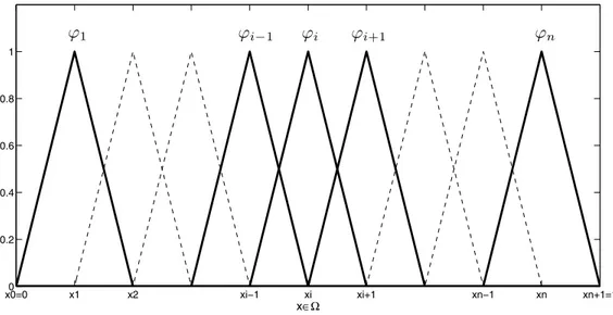
Moreover, we consider the hat-functions (see Figure 1) as the piecewise linear basis functions {ϕi}ni=1given by
ϕi(x) =
x−xi−1
h , xi−1≤x≤xi, xi+1−x
h , xi≤x≤xi+1, 0, otherwise.
(3.3)
Using this finite element formulation (or this discrete variational formulation) [2, 6], approximating the solution of (3.1) consists in obtaininguh∈V0
h, such that
✂ 1
0
u′h(x)v′(x)dx=
✂ 1
0
x0=00 x1 x2 xi−1 xi xi+1 xn−1 xn xn+1=1 0.2
0.4 0.6 0.8 1
x∈Ω
ϕ
1ϕ
i−1ϕ
iϕ
i+1ϕ
nFigure 1: Piecewise linear basis functions ofVh0.
Using the basis functions ofVh0(ϕj∈Vh0),uhis given by a linear combination of functionsϕj
[2, 6], with coefficientsξjsuch that
uh(x) = n
∑
j=1
ξjϕj(x) and u′h(x) = n
∑
j=1
ξjϕ′j(x). (3.4)
Sinceuh(x)in (3.4) is an approximation tou(x), we have
n
∑
j=1
ξj ✂ 1
0
ϕ′j(x)v′(x)dx
=
✂ 1
0
f(x)v(x)dx,∀v∈Vh0.
Taking v(x) =ϕi(x), for each i=1,2, ..,n, we can find ξj, for j=1,2, ...,n, by solving the
following system of linear equations
n
∑
j=1 ✂ 1
0
ϕ′j(x)ϕi′(x)dx
ξj=
✂ 1
0
f(x)ϕi(x)dx, i=1,2, ... ,n.
Thus, we have a discrete problem represented by a linear system of equations [2, 6], that can be given in the matrix form as
Aξ =b, (3.5)
whereA= [ai j]ni,j=1∈Rn×n, with
ai j=
✂ 1
0
ξ = [ξj]nj=1∈Rn, andb= [bi]ni=1∈Rn, with
bi=
✂ 1
0
f(x)ϕi(x)dx. (3.7)
If we assume the basis functions (3.3), then{ϕi′}n
i=1are defined, fori=1,2, ...,n, as follows:
ϕi′(x) = 1
h, xi−1≤x≤xi, −1h, xi≤x≤xi+1,
0, otherwise.
Thus, the coefficients of matrixA, described above in (3.6), are given by
aii=
✂ 1
0
ϕi′(x)ϕi′(x)dx=
✂ xi
xi−1 1 h· 1 h dx+
✂ xi+1
xi −1 h · −1 h
dx=2
h, (3.8)
fori=1,2, ...,n, and
ai,i−1=
✂ 1
0
ϕi′(x)ϕi′−1(x)dx=
✂ xi
xi−1 1 h· −1 h
dx=−1
h, (3.9)
fori=2,3, ...,n.
SinceAis symmetric, we have thatai−1,i=ai,i−1and by the definition of the basis we conclude
thatai j=0 for|i−j|>1.
Thus, we may obtain vectorb in (3.7), by using the simple trapezoidal rule to approximate a numerical integration:
bi =
✂ 1
0
f(x)ϕi(x)dx=
✂ xi
xi−1
f(x)ϕi(x)dx+
✂ xi+1
xi
f(x)ϕi(x)dx
=
✂ xi
xi−1
f(x)x−xi−1 h dx+
✂ xi+1
xi
f(x)xi+1−x
h dx (3.10)
≈ xi−xi−1 2 f(xi) +
xi+1−xi
2 f(xi) =h f(xi).
Thus, if f(xi) = fifori=1,2, ...,n, then the final configuration of system (3.5) is
A=1 h
2 −1 0 ··· 0
−1 2 −1 . .. ...
0 −1 2 . .. 0 ..
. . .. ... ... −1 0 ··· 0 −1 2
, ξ =
ξ1 ξ2 .. .
ξn−1
ξn
and b=h
f1 f2 .. . fn−1
fn .
Finally, coefficientsξj are obtained and the approximate solutionuh, which depends strongly
on the the function f, is determined. The functionuhcorresponds to the numerical solution of a
BVP (3.1) by the FEM [2].
4 ADAPTATION OF THE SUGENO INTEGRAL
Definition 4.1 (Sugeno Integral).[9, 12]Let f : Ω→[0,1]be a function andµe a normalized fuzzy measure onΩ. The Sugeno integral of f with respect toµeis given by
✥
Ω
f dµe = sup α∈[0,1]
[α∧H(e α)], (4.1)
where∧is the minimum operator andH(e α) =µe{x∈Ω: f(x)≥α}is called the level function of f[3].
Theorem 1. [3, 12]Let f: Ω→[0,1]be a function (typically a membership function) andµea normalized fuzzy measure onΩ.If
e
H(α) =µe{x∈Ω: f(x)≥α}
has a fixed pointα, then ✥
Ω
f deµ = α = H(e α).
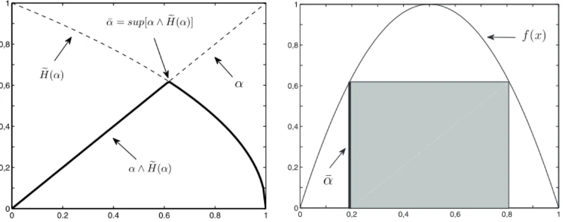
In [1], a theoretical and applied study in fuzzy measures and integrals is presented. It also states that the Sugeno integral can be interpreted geometrically as the side of the greatest inscribed square between the integrated function and thex−axis (see Figure 2b).
For example, we can consider the function f :Ω→[0,1]defined by f(x) =−4x2+4x. Thus, f is a typical membership function of a fuzzy subsetFofRwhoseα-levels are given by
[F]α={x∈R:−4x2+4x≥α}=
1−√1−α
2 ,
1+√1−α
2
.
Ifµis the usual Lebesgue measure (2.2) onΩ=R, then the level functionH(e α)is
e
H(α) =µ([F]α) =1+
√ 1−α
2 −
1−√1−α
2 =
√ 1−α.
Therefore, according to (4.1), the Sugeno integral can be written as:
✥
Ω
f dµe = sup α∈[0,1]
[α∧√1−α].
SinceH(e α)is a decreasing function, we have
✥
Ω
f dµe = α = H(e α) = −1+ √
5
sinceα=√1−α=⇒α=−1+√5
2 ≈0.61803.
The function f, the level functionH(e α)and the result obtained by the Sugeno integral are shown in Figure 2a and 2b.
0 0.2 0.4 0.6 0.8 1 0
0,2 0,4 0,6 0,8 1
α
¯
α=sup[α∧He(α)]
e
H(α)
α∧He(α)
0 0,2 0,4 0,6 0,8 1
0 0,2 0,4 0,6 0,8 1
¯ α
f(x)
Figure 2: Sugeno integral: (2a) The fixed point of H(e α)and (2b) Geometric interpretation of (4.1).
As mentioned in [7], the Sugeno integral was defined only for functions whose range is con-tained in [0,1] and for normalized fuzzy measures. As we can note in the previous exam-ple, the Sugeno integral is considered a good approximation to the Riemann integral (because
✁1
0 f dx=2/3≈0.66667). However, in [8], it was mentioned that the use of the Sugeno integral
for functions whose range is contained in[0,k],k>0. But, whenk6=1 or the fuzzy measureµis not normalized, the Sugeno integral may not be a good approximation to the Riemman integral (see examples in [10]).
We established an adapted fuzzy integral based on the Sugeno integral and with respect to a finite fuzzy measure. This integral approximates the Riemann integral for any functions whose range is in[0,k], withk∈R+.
Definition 4.2 (Adapted fuzzy integral).Let f :Ω→[0,k]be a measurable function such that
k=supx∈Ω f(x). The adapted fuzzy integral of f onΩ, with respect to the finite fuzzy measure
µ:A →[0,∞), that is,µ(Ω)<∞, is given by
c
✥
Ω
f dµ =
(
kµ(Ω)✤Ω bf deµ ,if k>0
0 ,if k=0 (4.2)
where bf(x) = f(kx) for all x∈Ω, andµe(B) =µµ((ΩB)) for all B∈A.
Next, we establish another representation of (4.2) and we present a numerical integration formula to calculate it.
First, from (4.2) and (4.1), we have that
✥
Ω b
f deµ = sup α∈[0,1]
h
α∧Hbe(α)i, (4.3)
where
be
H(α) = eµ{x∈Ω: bf(x)≥α} = µe{x∈Ω: f(x)≥kα}
= µ{x∈Ω: f(x)≥kα}
µ(Ω) =
H(kα)
µ(Ω) (4.4)
andH(β) =µ{x∈Ω: f(x)≥β}.
Thus, according to Theorem 1 and Equation (4.4), we have that the value of (4.3) is given by
✥
Ω b
f deµ = α = H(be α) = H(kα)
µ(Ω) .
Takingβ=kα, we have that
α = β k =
H(β)
µ(Ω). (4.5)
Therefore, another representation of (4.2), fork>0, is given as
c
✥
Ω
f dµ = kµ(Ω)α = µ(Ω)β = k H(β).
Thus, from Equation (4.5), the calculus of the adapted fuzzy integral boils down to solving the equationβ=µ(kΩ)H(β).
In what follows we provide a numerical integration formula to approximate the Riemann integral, over[a,b]⊆R+, of differentiable and increasing functions.
Let f :Ω→R+ be a differentiable and increasing function. The Riemann integral of f over
Ω= [a,b]is approximated by
SΩ(f) =d f(a) +
dc2
c+d f′(b), (4.6)
Note that
✂ b
a
f(x)dx =
✂ b
a
f(a)dx+
✂ b
a
(f(x)−f(a))dx
≈ (b−a)f(a) +c
✥
Ω
g dµ
= d f(a) +cµ(Ω)
✥
Ω b
g dµe.
≈ d f(a) + dc
2
c+d f′(b)=SΩ(f).
The value✤bΩg dµ=dβ ≈ dc2
c+d f′(b) is obtained as follows. From (4.5), we have
β = c H(β)
µ(Ω) = c dµ
h
g−1(β),bi=c d
b−g−1(β)
Fromg(g−1(β)) =gb−dβ
c
and using first-order Taylor series aboutb, we obtainβ≈g(b)−
dβ
c g′(b)and, therefore,
β≈ g(b) 1+d gc′(b) =
f(b)−f(a)
c+d f′(b)
c
= c
2
c+d f′(b).
The next theorem establishes that formula (4.6) coincides with the Riemann integral of certain power functions.
Theorem 2.Let f :Ω→R+be a power function given by f(x) =c1xn+c2with c1, c2, n∈R+,
and letµbe an usual Lebesgue measure inΩ= [0,b]. We have
✂ b
0
f(x)dx=SΩ(f).
Proof. On the one hand, we have that
✂ b
0
f(x)dx=
✂ b
0
(c1xn+c2)dx=
c1
xn+1
n+1+c2x
b
0
=c1
bn+1
n+1+c2b.
On the other hand, from (4.6) we get
SΩ(f) =b f(0) + b(c1
bn)2
c1bn+bnc1bn−1
=bc2+
b(c1bn)2
c1bn(1+n)
=bc2+c1
A consequence of Theorem 2 forΩ= [a,b]⊆R+is that
✂ b
a
(c1xn+c2)dx =
✂ b
0
(c1xn+c2)dx−
✂ a
0
(c1xn+c2)dx
= S
[0,b](c1x
n+c
2)− S [0,a](c1x
n+c
2)
= b f(0) + b(f(b)−f(0))
2
(f(b)−f(0)) +b f′(b)
−a f(0)− a(f(a)−f(0))
2
(f(a)−f(0)) +a f′(a).
5 NUMERICAL APPROACH AND SIMULATIONS
In the following example, we use the numerical integration formula (4.6) to calculate all the required elements for the matrix system (3.5) and, thus, to approximate the solution of the BVP (3.1) via FEM using an adapted fuzzy integral (4.2) based on the Sugeno integral.
First, in the elementsai,iof the matrixA, withΩi= [xi−1,xi], and using equidistant nodesd=h
andc=0, we have
aii =
✂ xi
xi−1
1 h2dx+
✂ xi+1
xi
1 h2dx
= SΩi
1 h2
+SΩi+1
1 h2
= 1
h + 1 h =
2
h. (5.1)
Thus, we observe that the entriesaiiof the matrixAgiven in (3.8) coincide with those obtained
by our proposal in (5.1).
Second, using the adapted fuzzy integral to determine the entriesai,i−1=ai−1,iof matrixA, we
haved=h,c=0, and
ai,i−1 = −
✂ xi
xi−1
1
h2dx= −SΩi
1 h2
= −1h. (5.2)
One can observe that the coefficientsai,i−1=ai−1,iobtained via the classical integration in (3.9)
and the our formula (5.2) are equal. By definition of the basis, we have thatai j=0 for|i−j|>1
Finally, the load vectorbis obtained using the numerical integration formula (4.6) for increasing functions f(x)andg(x) =x f(x), fori=1,2, ...,n:
bi =
✂ xi
xi−1
f(x)
x
−xi−1
h
dx+
✂ xi+1
xi
f(x)
x
i+1−x
h
dx
= 1
h
"✂ x i
xi−1
x f(x)dx−(xi−1)
✂ xi
xi−1
f(x)dx+ (xi+1)
✂ xi+1
xi
f(x)dx
−
✂ xi+1
xi
x f(x)dx
≈ 1hSΩi(g)−(xi−1)SΩi(f) + (xi+1)SΩi+1(f)−SΩi+1(g)
.
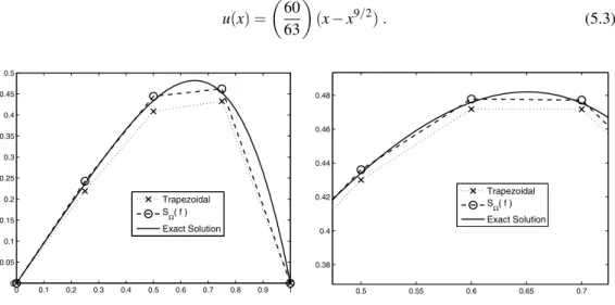
In order to illustrate the good results of formula (4.6), we solve the BVP in (3.1) taking the load function f(x) =15x2√x. This yields the exact solution which satisfies the boundary values given by
u(x) =
60 63
(x−x9/2). (5.3)
0 0.1 0.2 0.3 0.4 0.5 0.6 0.7 0.8 0.9 1 0
0.05 0.1 0.15 0.2 0.25 0.3 0.35 0.4 0.45 0.5
Trapezoidal SΩ( f ) Exact Solution
0.5 0.55 0.6 0.65 0.7 0.38
0.4 0.42 0.44 0.46 0.48
Trapezoidal SΩ( f ) Exact Solution
Figure 3: Graphs of the analytic solution for the BVP in (3.1) with f(x) =15x2√x, and the numerical solutions obtained by FEM using the trapezoidal rule andSΩ(f).
In Figure 3a and Figure 3b, we can see the analytical solution (5.3) as well as the numerical solutions obtained by numerical integration based on the trapezoidal rule (3.10) and by applying the formula (4.6). In this case, fori=1,2, ...,n, we considerxi=ihto divide the domain[0,1]
for both cases.
Table 1 shows the errorsE(xi) =Uaprox(xi)−u(xi), for different values ofn, between the
numer-ical solutionsUaprox(xi)and the exact solutionu(xi). Here, we consider the infinity norm and the
2-norm [5]:
||E||∞= max
1≤i≤n|E(xi)|,and||E||2= s
n
∑
i=1
Table 1: Errors between the numerical solutions and the exact solution of BVP in (3.1), with f(x) =15x2√x.
Partition Integration ||E||∞ ||E||2
n=3, h=1/4 Trapezoidal 2.5378×10−
2 3.6953×10⁻²
Adap. Fuzzy Int. 1.0396×10⁻² 1.5092×10⁻²
n=9, h=1/10 Trapezoidal 4.0441×10
−3 9.3259×10⁻³
Adap. Fuzzy Int. 1.9478×10⁻³ 4.4831×10⁻³
6 FINAL CONSIDERATIONS
In this paper, we introduced the notion of an adapted fuzzy integral based on the Sugeno integral. In addition, we propose a numerical integration formula (4.6) for differentiable, increasing, and non-negative functions whose range is contained in [0,k]. We verified that, under certain conditions, our proposal yields error equal to zero for power functions, according to Theorem 2. In initial simulations, the numerical solution of a BVP via FEM using our approach obtained better results than a well-known numerical integration method, namely trapezoidal rule (see Figure 3 and Table 1).
ACKNOWLEDGMENT
This work was partially supported by CONICYT of Chile, CNPq under grant n. 306546/2017-5 and n. 142380/2016-4, and Fapesp under grant n. 2016/26040-7.
RESUMO. Nessa proposta estudamos e definimos uma integral fuzzy adaptada, baseada na integral de Sugeno. Ademais, apresentamos uma f´ormula de integrac¸˜ao num´erica que aproxima o valor da integral fuzzy adaptada. Assim, provamos que a integral de Riemann e a integral fuzzy adaptada s˜ao equivalentes para func¸˜oes potˆencia. Logo, aplicamos a f´ormula proposta na integrac¸˜ao num´erica, requerida no m´etodo de elementos finitos, para obter uma soluc¸˜ao aproximada de um problema de valor de contorno para a equac¸˜ao de Poisson uni-dimensional. Finalmente, observamos melhores resultados na soluc¸˜ao aproximada obtida com o uso da nossa f´ormula quando comparada com a regra simples de trap´ezio.
Palavras-chave: Medida Fuzzy, Integral de Sugeno, M´etodo de Elementos finitos, Pro-blema de Valor de Contorno.
REFERENCES
[1] G. Arenas-Di´az & E.R. Ram´ırez-Lamus. Medidas difusas e integrales difusas. Universitas Scientiarum,18 (1)(1) (2013), 7–32.
[3] L.C. Barros, R.C. Bassanezi & W.A. Lodwick. A First Course in Fuzzy Logic, Fuzzy Dynamical Systems, and Biomathematics. Springer, New York (2017).
[4] L.T. Gomes, L.C. Barros & B. Bede. Fuzzy Differential Equations in Various Approaches. SBMAC SpringerBriefs. Springer, New York (2015).
[5] R.J. Leveque. Finite difference methods for ordinary and partial differential equations - steady-state and time-dependent problems. SIAM (2007).
[6] J. Li & Y. Chen.Computational Partial Differential Equations Using MATLAB. CRC Press Taylor & Francis Group (2008).
[7] T. Murofushi & M. Sugeno. Fuzzy measures and fuzzy integrals. Fuzzy Measures and Integrals: Theory and Applications, (2000), 3–41.
[8] H. Nguyen & E. Walker.A First Course in Fuzzy Logic. CRC Press Taylor & Francis Group (2006). [9] W. Pedrycz & F. Gomide.Fuzzy systems engineering toward human-centric Computing. IEEE Press.
John Wiley & Sons, New Jersey, EUA (2007).
[10] H. Rom´an-Flores, A. Flores-Franulic & Y. Chalco-Cano. The fuzzy integral for monotone functions.
Applied Mathematics and Computation,185(1) (2007), 492–498.
[11] D. S´anchez, L.T. Bassani, L.C. Barros & E. Esmi. Ensaios do M´etodo de Elementos Finitos com Integral Fuzzy. In Proceedings of IV CBSF. Recentes Avanc¸os em Sistemas Fuzzy, SBMAC (2016). [12] M. Sugeno. Theory of fuzzy Integrals and Applications. Ph.D. thesis, Tokyo Institute of Technology
(1974).
[13] L.A. Zadeh. Information and control.Fuzzy sets,8(3) (1965), 338–353.
APPENDIX
Table 2 presents some numerical results using the numerical integrationSΩ(f)(formula (4.6)
based on the adapted fuzzy integral) for differentiable and increasing functions in the interval
Ω= [0,1]. The results are compared with others numerical integration rules such as midpoint
IMP(f), trapezoidal ITra(f)and SimpsonISim(f). The reference value was obtained using the
Gauss Quadrature ruleIGQ(f)≈
✁b
a f(x)dx, which is an optimal numerical approximation which
requires a resolution of a linear system of equations for each integration [2, 5].
Table 2: Absolute errors obtained using several rules of numerical integration, and by (4.6).
f(x) IGQ(f) ISim(f) ITra(f) IMP(f) SΩ(f)
ex4 1.27129 1.3294 1.8591 1.0645 1.2345
Error - 5.8087×10⁻² 5.8785×10⁻¹ 2.0680×10⁻¹ 3.6805×10−2
x5sin(x) 0.12508 0.15023 0.42074 0.014982 0.12669
Error - 2.5152×10⁻² 2.9565
×10−1 1.1010
×10−1 1.6065 ×10⁻³
15x2√x 4.2857 4.2678 7.5000 2.6517 4.2857
![Table 2 presents some numerical results using the numerical integration S Ω ( f ) (formula (4.6) based on the adapted fuzzy integral) for differentiable and increasing functions in the interval Ω = [0, 1]](https://thumb-eu.123doks.com/thumbv2/123dok_br/16169945.707699/13.744.155.630.830.951/presents-numerical-numerical-integration-integral-differentiable-increasing-functions.webp)
