The Effect of Numerical Integration on the Finite Element Approximation of a Second Order Elliptic Equation with Highly Oscillating Coefficients

(1)

Available online at www.ispacs.com/jiasc

Volume 2015, Issue 2, Year 2015 Article ID jiasc-00084, 9 Pages doi:10.5899/2015/jiasc-00084

Research Article

The Effect of Numerical Integration on the Finite Element

Approximation of a Second Order Elliptic Equation with

Highly Oscillating Coefficients

Bienvenu Ondami∗

Universite Marien NGOUABI, Facult´ e des Sciences et Techniques, BP. 69, Brazzaville, Congo.´

Copyright 2015 c⃝Bienvenu Ondami. This is an open access article distributed under the Creative Commons Attribution License, which permits unrestricted use, distribution, and reproduction in any medium, provided the original work is properly cited.

Abstract

In this paper, we have studied the effect of numerical integration on the Finite Element Method (FEM) based on the usual Ritz approximation using continuous piecewise linear functions, in the context of a class of second order elliptic boundary value problems with highly periodically oscillating coefficients. An error estimate depending onε

the parameter involved in the periodic homogenization andhthe mesh size is established. Numerical results for one dimensional problem are presented. It is shown that when_εhis a positive integer then the method gives different re-sults depending on the shape of the coefficients and the numerical integration. Specifically we obtain perfectly correct results in some cases and completely false in other cases.

Keywords:Numerical Integration, Homogenization, Elliptic Equations, Finite Elements.

1 Introduction

There are many practical computational problems with highly oscillatory solutions e.g. computation of flow in heterogeneous porous media for petroleum and groundwater reservoir simulation (see, e.g.,[8] and the bibliographies therein). If a porous medium with a periodic structure is considered, with the size of the period is small enough compared to the size of the reservoir, and denoting their ratio byεan asymptotic analysis, as ε−→0,is required. Using the homogenization tools (see, e.g.,[3], [4], [9], [12]) the original equation describing this problem can be replaced by an effective or homogenized equation modeling some average quantity without the oscillations.

Whenever effective equations are applicable they are very useful for computational purposes. There are however many situations for whichεis not sufficiently small so that the effective equations are not practical. In this cases the original equation has to be approximated directly.

When the approximation is done by a finite element method, numerical integration is almost unavoidable. In this paper we will study the effect of numerical integration when a finite element method is used to approximate the original equation. Specific problems considered here include a linear elliptic equation in divergence form with highly periodically oscillating coefficients. The purpose of this paper is to show that even whenh_ε is an integer the numerical solution with numerical integration effects can be correct in some cases depending on the shape of coefficients. The numerical approximation partial differential equations with highly oscillating coefficients has been a problem

∗_{Corresponding author. Email address: bondami@gmail.com, Tel: +242 069242063}

(2)

of interest for many years and many methods have been developed (see, e.g., [1], [6], [7], [10], [11], [13] and the bibliographies therein).

The paper is organized as follows. In section 2 we have given a short description of the boundary value problem used in this study and the classical homogenization result related to this problem. In section 3, the conforming finite element method with numerical integration of the problem is presented as well as an error estimate. Numerical simulations for the one-dimensional problem comparing the approximation obtained by that method and the approximation of the homogenized problem are presented in section 4. Lastly, some concluding remarks are presented in section 5.

2 Preliminaries and notations

LetΩ⊂Rn(n=1,2)be a bounded polygonal convex domain with a periodic structure and smooth boundaryΓ. More precisely, we shall scale this periodic structure by a parameterεwhich represents the ratio of the cell size to the

size of the whole regionΩand we assume that 0<ε<<1 in a decreasing sequence tending to zero. LetY =∏n

i=1

]0,yi[ representing the microscopic domain of the basic cell. Assume that in such a configuration the absolute permeability tensor depends only on the microscopic variabley= x

ε wherexis the variable in the macroscopic scale. Namely

Kε(x) =K(x

ε)withKisY−periodic function onY.LetSbe the space of symmetric tensors. For two elementsAand

BinS, we introduce a partial ordering6such thatA_≤Bif and only if

<A−→ξ,−→ξ >6<B→−ξ,−→ξ >,∀−→ξ _∈Rn,

where< ., . >denotes the standard inner product onRn.We define the set of bounded, measurable, uniformly positive definite tensor onΩby

M(α,β;Ω):={A_∈L∞(Ω;S) /αI_≤A_≤βI a.e.inΩ},

whereαandβ are positive constants such thatα≤β. Throughout the paper, we use the Sobolev spaces

Hm(Ω) ={

v_∈L2(Ω), ∂αv_∈L2(Ω), ∀|α| ≤m} ,

with the multi-index(α1,α2, ...,αn), |α|:= ∑n

i=1

αi,and∂α:=∂α1∂α2...∂αn.TheHm−norm and semi-norm of any

v_∈Hm(Ω)are respectively defined by

∥v_∥2_m_,_Ω:=

_∑

|α|≤m

∥∂αv_∥2_L2_(Ω),

|v_|2_m_,_Ω:=

_∑

|α|=m

∥∂αv_∥2_L2_(Ω),

while theL2₋norm is

∥v_∥2_L2_(Ω)=

∫

Ω|v|

2_dx_.

In addition, we denote byH₀1(Ω)⊂H1(Ω)the subspace consisting of zero-trace functions. We also use the space

W1,∞(Ω)equipped with the norm∥.∥∞,Ω. We consider the following elliptic boundary value problem: (Pε)

{

−div(Kε(x)▽uε) = f inΩ,

uε = 0 onΓ,

wheref is a function inL2₍_Ω₎_._If_K_∈_M₍_α_,_β_;_Ω₎_then_Kε_∈_M₍_α_,_β_;_Ω_{). By homogenization theory (see, e.g.,[4],[9],} [12] ), it follows that

(3)

whereusatisfies the following homogenized equation,

(P0)

{

−div(K∗▽u) = f inΩ,

u = 0 onΓ,

and the entries of the matrixK∗are given by

(K∗)_{i j}= 1

|Y| ∫

Y

K(y) [∇wi+−→ei].[∇wj+−→ej] 1≤i,j≤n,

withwj,j=1, . . . ,nis the solution of the so-called local or cell problem defined by:

{

wj∈Hp1(Y)/R,

−div[K(y) (∇wj+−→ej)] = 0 inY.

Here−→ej is the jthstandard basis vector ofRn.We denote byC∞p(Y)the space of infinitely differentiable functions in Rnthat are periodic of periodY.ThenH1_p(Y)is the completion for the norm ofH1(Y)ofC∞_p(Y).

The effective tensorK∗is still symmetric and positive definite but in general cases, even with the permeability at the microscopic scale in the porous medium being isotropic, we may have an effective tensor which is significantly anisotropic. In porous medium flow, the problem(Pε)results from Darcy’s law and continuity for a single phase, incompressible flow through a horizontal heterogeneous porous medium with periodic structure.

3 The Finite Element Approximation with Numerical Integration

The variational form of the problem(Pε)is given as

{

uε∈H01(Ω),

a(uε,v) =∫ΩKε(x)uεvdx=∫Ωf vdx ∀v∈H01(Ω).

(3.1)

We will make the following assumptions: (A1)Kε_∈M(α,β;Ω),

(A2)Kε_∈W1,∞(Ω), (A3) f _∈L2(Ω).

It is well known that (3.1) has a unique solutionuε∈H2(Ω)∩H01(Ω). The finite element method:Let(T_h)

h>0be a regular triangulation ofΩwherehis the mesh size, and let V_h={v_h; v_h_∈C0(

Ω)

,v_his affine on eachT _∈T_h_,v_h=0 onΓ}

be the finite element subspace. The finite element approximation to the solutionuε∈H01(Ω)of (3.1) is given by the

finite method (FEM),

{

uεh∈Vh,

a(uεh,vh) =f(vh) ∀vh∈Vh (3.2)

wheref(vh) =∫

Ω f vhdx.The following error estimate is well-known, see, e.g., [1], [10]:

|uε−uεh|1,Ω≤C h

(

1+1

ε )

. (3.3)

Note thata(uεh,vh)and f(vh)contain definite integrals that can be computed numerically. Consequently, the FEM with numerical integration is given by

{

u∗_εh_∈Vh,

(4)

wherea∗(., .)andf∗(.)are the computation results by numerical integration ofa(uεh,vh)and f(vh)respectively. In almost all finite element compilation, numerical integration is unavoidable. Consequently,u∗_εhinstead ofuεhis available. Throughout the paper, we denote byC generic constants, even if they take different values at different places.

We now state the main result of this section.

Theorem 3.1. Assume that the quadrature rules for computing a∗(., .)and f∗(.)are exact on all polynomials of degrees less than or equal to1and let f_∈H2(Ω).Then the following estimate is valid:

∥uε−u∗εh∥1,Ω≤C h

(

1+1

ε )2

(3.5)

where C is a constant independent ofεand h.

Proof. We do the proof forn=2 (two-dimensional). The proof of this result is obtained by using [2, Theorem 2.1]

and [5, Theorem 4.1.6]. Indeed, these theorems imply

∥uε−u∗εh∥1,Ω≤Ch

( 2

∑

i,j=1

K_{i j}ε_∞_,_Ω∥uε∥2,Ω+∥f∥2,Ω

)

(3.6)

whereCis a constant independent ofεandh.Now we are going to estimate the term

2

∑

i,j=1

K_{i j}ε_∞

,Ω∥uε∥2,Ω.

Using [1, Theorm 2], we deduce that

∥uε∥2,Ω≤C

(

1+1

ε )

whereCis a constant independent ofε.By the definition of∥.∥∞,Ωwe have

K_{i j}ε

2

∞,Ω=

Ki j

(x₁ ε, x2 ε ) 2

L∞_(Ω)+

∂Ki j

(x₁ ε,

x2 ε

)

∂x1 2

L∞(Ω) +

∂Ki j

(x₁ ε,

x2 ε

)

∂x2 2

L∞(Ω)

,∀ i,j=1,2.

Therefore we get

K_{i j}ε

2

∞,Ω=

K_{i j}ε

2

L∞(Ω)+ 1 ε2

∂K_{i j}ε ∂x1 2

L∞_(Ω) + 1 ε2

∂K_{i j}ε ∂x2 2

L∞_(Ω)

,∀ i,j=1,2,

K_{i j}ε

2

∞,Ω≤C

(

1+ 1

ε2 )

≤C (

1+1

ε )2

.

Finally, we deduce that

K_{i j}ε_∞

,Ω≤C

(

1+1

ε )

.

Thus, we obtain

2

∑

i,j=1

K_{i j}ε_∞_,_Ω∥uε∥2,Ω≤C

(

1+1

ε )2

.

We can now deduce that

2

∑

i,j=1

K_{i j}ε

∞,Ω∥uε∥2,Ω+∥f∥2,Ω≤C

(

1+1

ε )2

(5)

So

∥uε−u∗εh∥1,Ω≤Ch

(

1+1

ε )2

,

which is the desired result. ✷

Remark 3.1. For the one-dimensional problem, the result of theorem 3.1 could be obtained by simple calculations. Furthermore, the error estimate for higher order approximation is easy to be derived like in [10].

4 Numerical Results

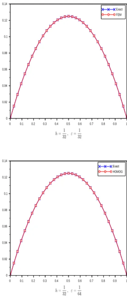
In this section we present numerical results for one-dimensional problem comparing the finite element method described in this paper and the example of exact solution and homogenized solution(HOMOG). In this case the homogenized coefficient is computed as the harmonic mean. In the first example, we compare the approximate solution to the exact solution and the homogenized solution.The results obtained are pefectly correct even whenh_ε is a positive integer. In the second example, we compare the approximate solution to the homogenized solution. The results obtained show that the approximate solution is false whenh_ε is a positive integer.

The first test problem involved simulation with the coefficient:

K(y) = 1

a+bsin(2πy), 0<b<a, y∈[0,1],

and

f =1.

In this case, the exact solution is:

uε(x) =−

ax2

2 +

[

aC₁ε+bε 2πcos

(

2πx ε

)]

x₋bε

2π [

Cε₁cos

(

2πx ε

)

+ ε

2πsin (

2πx ε

)]

+C₂ε, (4.7)

where

Cε₁= a

2−

bε

2π

[

cos(2π ε

)

−2επsin

(2π ε

)]

a+₂bε_π[

1−cos(2π ε

)] ,

and

Cε₂= bε 2πC

ε

1.

The homogenized solution is:

(6)

0 0.1 0.2 0.3 0.4 0.5 0.6 0.7 0.8 0.9 1 0

0.1

0.02 0.04 0.06 0.08 0.12 0.14

Exact FEM

0 0.1 0.2 0.3 0.4 0.5 0.6 0.7 0.8 0.9 1 0

0.1

0.02 0.04 0.06 0.08 0.12 0.14

Exact FEM

0 0.1 0.2 0.3 0.4 0.5 0.6 0.7 0.8 0.9 1 0

0.1

0.02 0.04 0.06 0.08 0.12 0.14

Exact FEM

0 0.1 0.2 0.3 0.4 0.5 0.6 0.7 0.8 0.9 1 0

0.1

0.02 0.04 0.06 0.08 0.12 0.14

Exact HOMOG

Figure 1: Test problem 1:a=1, b=1/2.

(7)

0 0.1 0.2 0.3 0.4 0.5 0.6 0.7 0.8 0.9 1 0

0.1

0.02 0.04 0.06 0.08 0.12 0.14

Exact FEM

0 0.1 0.2 0.3 0.4 0.5 0.6 0.7 0.8 0.9 1 0

0.1

0.02 0.04 0.06 0.08 0.12 0.14

Exact FEM

0 0.1 0.2 0.3 0.4 0.5 0.6 0.7 0.8 0.9 1 0

0.1

0.02 0.04 0.06 0.08 0.12 0.14

Exact FEM

0 0.1 0.2 0.3 0.4 0.5 0.6 0.7 0.8 0.9 1 0

0.1

0.02 0.04 0.06 0.08 0.12 0.14

Exact HOMOG

Figure 2: Test problem 1:a=1, b=1/2.

Those resultas show that whenh_ε is a positive integer the finite element approximation coincides with the exact solution and the homogenized solution. In fact this is due to the effect of numerical integration and the particular shape of the coefficient. Indeed we note that whenx_ε =m or x_ε=m₂,wheremis a positive integer,

Kε(x) =K(x ε )

=1

a,

which is none other than the harmonic mean of the coefficientK.Therefore the computation of integrals (3.4) by a numerical integration rule as trapezoid rule (the one we used in this paper) leads to the same equations that those obtained by replacingKεby1_a(see, [10]).

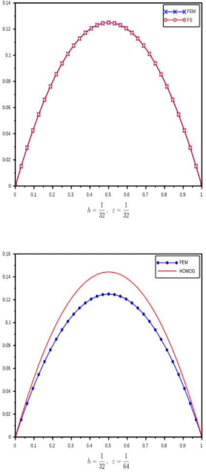
The second test problem involved simulation with the coefficient:

K(y) =1+0.5 sin(2πy), y_∈[0,1]

and

f =1.

In this case the homogenized solution is:

u(x) =√x

3(1−x).

By following the arguments of the first test problem, it is easy to see that the finite element approximation coincides with the solution obtained by replacingKε(x)by 1(arithmetic mean ofK). That solution (FS) is:

uf s(x) =x

(8)

That solution is called false because it has no link either with the homogenized solution or with the exact solution.

0 0.1 0.2 0.3 0.4 0.5 0.6 0.7 0.8 0.9 1 0

0.1

0.02 0.04 0.06 0.08 0.12 0.14

FEM FS

0 0.1 0.2 0.3 0.4 0.5 0.6 0.7 0.8 0.9 1 0

0.1

0.02 0.04 0.06 0.08 0.12 0.14

FEM FS

0 0.1 0.2 0.3 0.4 0.5 0.6 0.7 0.8 0.9 1 0

0.1

0.02 0.04 0.06 0.08 0.12 0.14 0.16

FEM HOMOG

0 0.1 0.2 0.3 0.4 0.5 0.6 0.7 0.8 0.9 1 0

0.1

0.02 0.04 0.06 0.08 0.12 0.14 0.16

FS HOMOG

Figure 3: Test Problem 2

5 Concluding remarks

The purpose of this paper was to help clarify the issue of the effect of numerical integration on the finite element approximation in the context of a class of second order elliptic boundary value problems with highly oscillating coefficients. An error estimate was obtained. In this paper the approximation has been done by continuous piecewise linear functions. Numerical results obtained here are still true for an approximation by continuous piecewise quadratic functions. Furthermore it is easy to see that all results obtained are still true if one consider a coefficients matrix of the shapeKε(x) =K(

x,x ε

)

,whereKisY-periodic.

Acknowledgements

I would like to thank the referee for the careful review and the valuable comments, which provided insights that helped improve this paper.

References

(9)

[2] I. Babuska, U. Banerjee, H. Li, The effect of numerical integration on the finite element approximation of linear functionals, Numer. Math, 117 (1) (2011) 65-88.

http://dx.doi.org/10.1007/s00211-010-0335-2

[3] N. Bakhvalov, G. Panasenko, Homogenization: processes in periodic media, Mathematics and its Applications, 36, Kluwer, Academic Publishers, London, (1989).

[4] A. Bensoussan, J. L. Lions, G. Papanicolaous, Asymptotic analysis for periodic structures, Studies in Mathe-matics and its Applications, 5, North-Holland, Amsterdan, (1978).

[5] P. G. Ciarlet, The finite element method for elliptic problems, Studies in Mathematics and Its Applications 4, North Holland, Amsterdam, (1978).

[6] Z. Chen, T. Y. Hou, A mixed multiscale finite element method for elliptic problems with oscillating coefficients, Mathematics of computation, 72 (242) (2003) 541-576.

http://dx.doi.org/10.1090/S0025-5718-02-01441-2

[7] W. M. He, J. Z. Cui, A new approximate method for second order elliptic problems with rapdly oscillating coefficients based on the method of multiscale asymptotic expansions, J. Math. Anal, 335 (1) (2007) 657-668.

http://dx.doi.org/10.1016/j.jmaa.2007.01.085

[8] U. Hornung, Homogenization and porous media, Interdisciplinary Applied Mathematics 6, Springer-Verlag, New York, (1997).

http://dx.doi.org/10.1007/978-1-4612-1920-0

[9] V. V. Jikov, S. M. Kozlov, O. A. Oleinik, Homogenization of differentials operators and integral functionals, Springer-Verlag,Berlin, (1994).

http://dx.doi.org/10.1007/978-3-642-84659-5

[10] B. Ondami, Sur quelques problèmes d’homogénéisation des écoulements en milieux poreux, Thèse de Doctorat, Université de Pau et des Pays de l’Adour, (2001).

[11] R. Orive, E. Zuazua, Finite difference approximation of homogenization problems for elliptic equations Multi-scale Model, simul, 4 (1) (2005) 36-87.

http://dx.doi.org/10.1137/040606314

[12] E. Sanchez-Palancia, Non-Homogeneous media and vibration theory, Lecture Notes in Physics, 127, Springer-Verlag, Berlin, (1980).

http://dx.doi.org/10.1007/3-540-10000-8

[13] H. Versieux, M. Sarkis, Convergence analysis for the numerical boundary corrector for elliptic equations with rapidly oscillating coefficients, SIAM J. Numer. Anal, 46(2) (2008) 545-576.