Main drivers of bank default situations

M

ASTER OF

S

CIENCE IN

M

ONETARY AND

F

INANCIAL

E

CONOMICS

M

ASTERS

F

INAL

W

ORK

D

ISSERTATION

M

AIN

D

RIVERS OF

B

ANK

D

EFAULT

S

ITUATIONS

F

RANCISCO

S

ALVADOR DE

P

AIVA

M

ASTER OF

S

CIENCE IN

M

ONETARY AND

F

INANCIAL

E

CONOMICS

M

ASTERS

F

INAL

W

ORK

D

ISSERTATION

M

AIN

D

RIVERS OF

B

ANK

D

EFAULT

S

ITUATIONS

F

RANCISCO

S

ALVADOR DE

P

AIVA

S

(

):

P

.

C

R

P

.

J

B

S

EPTEMBER

-

2014

Main Drivers of Bank Default Situations

Francisco S. Paiva

Supervisors: Clara Raposo, João Bastos Master in Monetary and Financial Economics

September 2014

Abstract

Since the 2007’s financial crisis we have witnessed an unprecedented number of financial institutions that either failed or had to be bailed out by the public sector. This work studies distress situations in financial institutions in the Euro area between 2001 and 2012, based on a data set with listed banks. The database is used to understand the main drivers for bank defaults, either financial (bank-specific) indicators, but also macroeconomic indicators are considered in the performed estimations. The main results show that both bank-specific and macroeconomic variables impact on default events. Capitalization, asset quality, market discipline, GDP growth rates and inflation rates are the most significant on the estimation results and should be taken into consideration when analyzing bank distress situations.

Table of Contents

1. INTRODUCTION ... 6

2. LITERATURE REVIEW ... 8

3. METHODOLOGY AND DATA ... 13

3.1.DATA DESCRIPTION ... 15 3.1.1. Defaults’ characterization ... 17 3.1.2. Explanatory variables ... 19 3.1.2.1. Capital ... 22 3.1.2.2. Asset Quality ... 23 3.1.2.3. Management ... 24 3.1.2.4. Earnings ... 24 3.1.2.5. Liquidity ... 25 3.1.2.6. Market Discipline ... 26 3.1.2.7. Growth ... 27

3.1.2.8. Macroeconomic environment factors ... 28

4. RESULTS AND DISCUSSION ... 31

5. CONCLUSION ... 36

REFERENCES ... 39

APPENDIX ... 40

APPENDIX DATA DESCRIPTION ... 40

DEFAULT CHARACTERIZATION ... 41

EXPLANATORY VARIABLES AVERAGE EVOLUTION ... 44

List of Figures and Tables

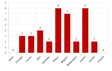
Figure 1 - Number of Defaults, by Country  ...  41  

Figure 2 - Number of Defaults, by Year  ...  42  

Figure 3 - Number of Defaults, by Year (% of total defaults)  ...  42  

Figure 4 - Total Equity to Total Assets sample average evolution  ...  44  

Figure 5 - Average of Loan Impairments to Total Net Loans (evolution)  ...  44  

Figure 6 - Average Cost-to-Income Ratio (evolution)  ...  45  

Figure 7 - Average Return on Equity (evolution)  ...  45  

Figure 8 - Average Return on Assets (evolution)  ...  45  

Figure 9 - Average of Liquid Assets to Total Assets (evolution)  ...  45  

Figure 10 - Average of Liquid Assets to Short-term Funding (evolution)  ...  45  

Figure 11 – Average Loan to Deposits ratio (evolution)  ...  45  

Figure 12 - Average Net Interest Income to Net Loans (evolution)  ...  45  

Figure 13 - Average Liabilities Growth Rates (evolution)  ...  45  

Figure 14 - Average GDP growth rate (evolution)  ...  46  

Figure 15 - Average Inflation rate (evolution)  ...  46  

Figure 16 – Average Government 10 year bonds’ interest rates (evolution)  ...  46  

Figure 17 - Average Balance of payments evolution (million euros)  ...  46  

Table I  ...  21 Table II  ...  32   Table III  ...  40   Table IV  ...  41   Table VI  ...  43   Table VII  ...  46   Table VIII  ...  47   Table IX  ...  47   Table X  ...  48   Table XI  ...  48   Table XII  ...  49   Table XIII  ...  49   Table XIV  ...  50  

1. INTRODUCTION

Since the 2007’s financial crisis we have witnessed an unprecedented number of financial institutions that either failed or had to be bailed out by the public sector. These bail out programs conducted by State-owned institutions were intended not only to avoid systemic risk, i.e. the risk of collapse of an entire financial system, but also to attempt to mitigate the negative effects of these bank failures in the real economy. Global banking crises, such as the 1890-91, 1907-08, 1913-14, 1931-32 and the one we have been witnessing (Bordo & Landon-Lane, 2010), have huge impact on economies leading to deep worldwide economic recession. Despite supervisory authorities around the world provided ample bailout programs to fragile banks, deposit guarantees to the general customer (to avoid bank runs) and highly expansionary monetary and fiscal policies, the world wide recession was inevitable, as a result of the credit crunch and the breakdown of the interbank market (Bordo & Landon-Lane, 2010). In Europe and particularly in the euro area, the lower economic performance could have affected the solvency of financial institutions, through big financial losses and lack of capacity from banks to absorb these external shocks.

Several bank failures occurred in Europe since 2008 with huge costs for taxpayers. Between 2008 and 2012, the overall volume of aid used for capital support (recapitalization and asset relief measures) amounted to €591.9 billion (4.6 % of EU 2012 GDP)1. Understanding the factors behind these failures is essential to empower supervisory authorities with the ability to prevent default situations in a more efficient way. The ability to predict failures or at least understand them would be a tremendous

gain in financial supervision and also to society in general, by avoiding the high bail out costs such as the ones we are witnessing nowadays.

This work studies the distress situations in financial institutions in the Euro area between 2001 and 2012, based on a data set with listed banks (in stock exchange indexes) from the euro area. The database is used to understand the main drivers for bank defaults, either financial (bank specific) indicators, or macroeconomic environment indicators.

Most of the existing literature focuses on the USA financial market and emerging markets (Kocagil, Reyngold, Stein, & Ibarra, 2002; Thomson, 1991). However, there is less literature on EU banks and even less in Euro area banks, since there did not exist many relevant bank distress situations until the recent crisis.

This work intends to provide a deep analysis on the comprehension of bank default situations across the Euro area in this recent financial and sovereign crisis. Contributing to a deep unprecedented insight of the recent Euro area’s banking crisis, of which there are few approaches.

Once the default situations are identified on the database, which exclusively occurred in the recent financial crisis, between 2008 and 2012, a panel data probit model is used in order to identify the main drivers of bank default situations. Using both bank specific and macroeconomic variables as possible distress variables. Bank specific indicators seem to be highly significant in determining distress situations during this financial turmoil. However, macroeconomic variables can also play a very relevant role on this quest, since banks are highly connected with the real economy’s performance (Thomson, 1991; Poghosyan & Cihak, 2011; Porath, 2006). The used methodology also wants to approach both impacts (bank-specific and macroeconomic variables) on bank default situations and also in bank’s performance, since there is no

consensus on whether macroeconomic variables impact on bank default situations. The approach confirms the relevance of both financial and macroeconomic variables on bank distress situations. Therefore, similar approach should be taken into consideration by the European authorities when analyzing bank default situations.

The structure of this work comprises a revision of the existing literature (section 2) on similar bank failure prudential models. Followed by section 3, where methodology and data are discussed, along with a description of how database was built and its main assumptions regarding distress situations. Section 5, shows the main results on the estimations and its discussion. Section 6 concludes, giving possible solutions to certain raised issues.

2. LITERATURE REVIEW

Despite the recent financial crisis around the world, studies related to prudential models on banking distress situations have been published well before the 2008 financial turmoil.

In 1974 Robert Merton proposed a model to evaluate the credit risk of a corporation’s debt by characterizing the corporate’s equity as a call option on its assets (Merton, 1974). Several extensions of this model in order to assess credit risk of companies have been developed (Black & Cox, 1976; Geske, 1977; Ahangarani, 2007). Despite the recognition of these structural models on corporate credit risk assessment, this approach may suffer from some limitations inherent in pricing methods when applied to financial institutions, since it ignores liquidity risk or transaction costs (Antunes & Silva, 2010).

Statistical prediction models were also developed before the recent financial crisis. Thomson (1991) studies bank failures in the 1980s with book data on US banks using a logit regression model. Through bank specific and macroeconomic variables, Thomson (1991) explains failure of the analyzed banks, where financial specific variables and economic conditions appear to affect the probability of bank failure. Most studies related with prediction of bank failures refer to U.S. banks, such as Moody’s RiskCalc™ Model for Privately-Held U.S. Banks, (Kocagil, Reyngold, Stein, & Ibarra, 2002), which covers the U.S. market from 1986-1999 including 17,673 banks and uses a probit estimation model.

The risk factors used to predict bank failure are related to different scopes of banking risk - capital, asset quality, concentration (on asset type), liquidity, profitability, growth and macro factors (Moody’s Trailing Speculative Default Rate

Index). To measure capital adequacy it is used the Equity capital / Assets ratio, which

is expected to have a negative impact (i.e. higher capital ratio means lower probability of default). For asset quality, the variables considered were Charge-Offs / Assets installments and Charge-Offs / Assets, their impact is expected to be positive, which means higher ratios leads to higher probabilities of default. The variables measuring concentration were Commercial Real Estate Loans / Assets, Construction Loans / Assets and C&I Loans / Assets, these are expected to have a positive impact in terms of probabilities of default, since higher ratios would mean lower diversification and higher exposure to a single sector. Liquidity (risk), which refers to the possibility of difficulties in meeting cash demands from current assets, is measured through Government Securities / Assets; its impact is expected to be negative, as a higher ratio would mean a higher percentage of liquid assets, meaning lower liquidity risk. Profitability is measured through Net Interest Income / Assets and is expected to have

a negative impact on probabilities of default. The growth variable (liabilities growth) is expected to have a positive impact on probabilities of default, because higher growth rate could suggest unsustainability of their management structure, and could mean the institution is measuring risk in an ineffective way. The macroeconomic variable reflects information on changes in credit quality in the financial markets, which is captured by Moody’s Trailing Speculative Default Rate Index; the impact is expected to be positive on probabilities of default of a bank. The final result is a model that the authors believe to be well suited to forecast future defaults. It could be viewed as a good aggregator of financial specific data that allows comparison between banking risks (Kocagil, Reyngold, Stein, & Ibarra, 2002).

However, we have observed an increasing number of related studies within the European financial institutions. Starting with German savings banks and cooperative banks, Porath (2006), covering for a period from 1993 to 2002, where a panel data binary model (logit, probit and log-logistic) is used, combining financial specific data and macroeconomic data. The studied (bank specific) variables follow a criterion similar to Kocagil, Reyngold, Stein, & Ibarra, (2002). As such, we could group the bank specific indicators into categories, the so called CAMEL variables, which stands for Capital (represented by Equity/Assets), Asset quality (Non-performing loans/total loans or loans loss provisions / total loans), Management (Cost-to-income ratio), Earnings (Operating results/ equity or EBIT/equity capital) and Liquidity (which was omitted from further analysis by the author due to lack of adequacy of the data). In terms of macroeconomic variables, Porath (2006) uses indicators for business cycles (such as GDP growth rate, money supply and unemployment) and macroeconomic prices (Interest rates and stock prices). The behavior of the chosen variables is similar to the previous mentioned study. The bank specific variables are similar, and so the

expected behavior is also identical. For macroeconomic variables the authors chose different variables, such as GDP growth rate, which is expected to have a negative impact on probabilities of default. On the other hand, interest rates, another macroeconomic environment chosen variable, are expected to have a positive impact on default probabilities, since higher interest rates can be interpreted as higher risk perception from investors. The expected behavior for stock prices is the opposite from that of the interest rates, with the same rationale. The results from this estimation demonstrate that general macroeconomic environment, bank’s return, asset quality variables and capitalization measures are significant determining the banks’ probabilities of default. The author also concludes that capitalization measures are the most relevant for the probabilities of default estimation, and that saving banks and cooperative banks are affected by the same risk factors (Porath, 2006).

Another example of a related study covering European banks is Poghosyan & Cihak (2011), which covers the period just before the recent financial crisis (1996 to 2007). The data used in the estimation of the probabilities of default (PDs) of individual banks is an extensive panel data for 5,708 European Union banks, estimated through a logistic probability binary model. The models in this study use not only bank specific CAMEL indicators, with indicators similar to those found in previous studies, but other potential determinants of banking risk, such as measures for market discipline (measured by the ratio of total interest expenses to total deposits) and measures to capture the clustering of bank failures (through a “dummy” contagion variable), where is captured to some extend the macroeconomic environment of the bank. The bank specific variables used in the performed model are similar to those used in the previous studies, and their behavior should be identical. The capitalization is measured as the ratio of total equity to total assets, lower ratio

would mean higher leverage, making the bank less resilient to certain shocks (sudden decrease in value of assets). Assets quality is measured through the ratio loan loss provisions to total loans (identical to those used the previous analyzed studies, and so similar behavior is expected). As a management quality parameter, the authors applied the cost-to-income ratio, which is the one used in the previous study, and a higher ratio would imply a weaker performance. To measure bank earnings the authors chose both ROE (Return on Equity ratio) and ROA (the Return on Assets ratio), which should impact negatively on the probabilitites of a bank default, suggesting that a higher return would mean lower distress probabilities. Liquidity, which is measured through the liquid assets to deposits and short-term funding, is expected to have a positive impact on the probabilities of a bank default, a lower ratio would imply a higher exposure to liquidity risk. The market discipline variable is expected to have a negative impact on the probabilities of a bank default in the sense that higher market discipline would suggest lower probabilities of distress, i.e. lower interest expenses to total deposits ratio. In the end, the model performance is satisfactory in classifying distressed banks, with capitalization, asset quality and earnings measures to be considered as statistically significant, as well as the measure for market discipline and the contagion variable.

In Poghosyan & Cihak, 2011 the market information (measured, for instance, by stock prices) appears to be relevant for predicting distressed situations. Market information is deeply explored in studies such as Curry, et al., 2003, suggesting that it contains relevant information on predicting distressed situations in financial instituions. Curry, et al. (2003) stated that publicly available information such as stock prices, returns and other market-related variables can provide timely information about the soundness of a financial institution. The authors also suggest that specially

equity market variables such as stock prices, returns, price volatility, market valuation, trading volume and share turnover improve the fit of the prediction model combined with traditional accounting data, as CAMEL indicators (Curry, Elmer, & Fissel, 2003).

The early developed models address the bank default risk in different ways, as it was previously mentioned. There is no consensus on the variables to be considered in the estimation models, and there are few studies performed with Euro area financial institutions. In this framework, the developed estimation models comprise Euro area banks, capturing the impact of both bank specific and macroeconomic variables. The recent financial crisis, namely in Europe and more specifically in the Euro area, raised important issues on supervision of banks. The soundness of financial system and the comprehension of how default situations trigger, are a great motivation to this work.

3. METHODOLOGY AND DATA

To evaluate the main drivers of a bank default event an econometric probit model using panel data is estimated. The panel data set allows the combination of bank specific with macroeconomic variables. The explained variable in the model will be the default of a bank, which is represented by a binary variable assuming the value 0 if the bank did not incur in default on the analyzed year, and the value 1 if the bank incurred in default on the analyzed year. To assign 0 or 1 to the default variable we need to define clearly the default event, i.e. under what conditions the bank is considered to default. We should take into consideration the fact that most banks do not completely bankrupt, due to state intervention programs (through capital injections or state guarantees and other forms of liquidity support) developed to avoid

systemic risk and to restore confidence in the financial sector, crucial to economic development. Thus, default is defined as any state or supervisory authorities’ intervention directly on capital, any kind of state guaranteed funding or asset purchase programs conducted by State owned institutions. The criteria behind this rationale results from the fact that a bank on these situations might not be able to meet international capital requirements by its own means or would not be able to fund its activities with market sources or, even worst, both situations. Another explanation for State intervention in banks may well result from stimulus creation to avoid credit crunch in the real economy.

This binary default variable will be the explained variable in the estimation probit model, through a set of different bank specific and macroeconomic variables.

Let 𝑌_!" be defined as the default variable of year t and from the specific bank j, and let 𝑋!" be the set of bank specific variables of the year t and the individual bank j.

Let 𝑍_!" represent the set of macroeconomic variables for the year t and the specific bank j. Considering these, we should have a panel binary response model given by:

(1) 𝑆_!,! =   𝛽_!+ 𝛽_!𝑋_!,!,! + ! 𝛽_!!!𝑍_!!!,!,!+  𝜀_!,!

!!! !

!!!

Where, 𝑆_!" is the score that is given to bank j in year t according to its set of bank-specific (𝑋_!") and macroeconomic (𝑍_!") variables. Regarding the bank specific variables the estimations will measure for the so-called CAMEL indicators (Capitalization, Asset quality, Management efficiency, Earnings and Liquidity) and other financial related variables (market discipline and growth), while macroeconomic variables will account for economic business cycles and for

macroeconomic prices. This estimation will use a probit random effects regression, which allows for individual effects. The signs of the 𝛽_! and 𝛽_!!!, coefficients give us the direction of the impact considering a marginal change in the explanatory variables on the probability of default. 𝛽_! is the constant coefficient that together with the link function described below, 𝜙(𝛽_!), gives the probability of default when the other explanatory variables are set to zero.

The probit implies a link function given by:

(2) 𝜙   𝑆!" = !_!! 𝑒

!!! !

!!,!

!! 𝑑𝑥

The probit link function (2) will give us the probability of default considering a specific 𝑆_!", which characterizes a given financial institution in a specific moment in time (year).

3.1. Data Description

The data set used to assess the main drivers on bank default is based on banks headquartered in the founding countries of euro area, covering from 2001 to 2012 (annual data). Due to complexity and bias of applying annual exchange rates to financial data, the database was restricted to banks headquartered in the founding countries of the euro area. Furthermore, the data set was restricted to stock exchange listed banks, as such the IBEX 35 (Spain), the PSI-20 (Portugal), CAC 40 (France), FTSE MIB (Italy), DAX-30 (Germany), ASE (Greece), BEL 20 (Belgium), AEX (Netherlands), ISEQ 20 (Ireland), ATX (Austria) and OMXH25 (Finland) were the considered indexes. The Luxembourg stock market index (the LuxX) was also

considered, however there is no listed bank besides the KBC Group, which has already been considered in the BEL 20 index. The fact that the euro area is a recently created monetary union, with a recent unprecedented financial crisis, makes the assessment of the drivers of bank defaults an interesting and relevant analysis, especially in the field of banking supervision.

The source of the financial individual data is the published annual reports of each financial institution. This selection criterion brought some problems on specific institutions, namely Unicredit whose the available financial information does not cover the whole period of the sample, and Media Banca, another Italian bank, wherein the financial information available is differently organized (financial year ends in July of each year) which could bias and lead to miscalculation problems in the sample. Thus, these two institutions were not considered in the sample.

Given this framework, the set of banks that were considered in the database are presented in table III of Appendix section. The sample contains 31 banks from 2001-2012, leading us to 372 observations.

3.1.1. Defaults’ characterization

The default characterization is one of the key issues of this analysis. The default selection criteria, mentioned above on the methodology section, brought several identified default situations. Figures 1, 2 and 3 of Appendix section show that most of bank failures resulted from the turbulent financial environment that began in 2008, affecting almost every European economy.

Every observed default (39 defaults) occurred between 2008 and 2012 and almost 50% of those defaults occurred in 2009, the year following the Lehman Brothers (US bank) bankruptcy. As shown in figure 1 (of Appendix section), no defaults were observed in Spain or in Finland. Despite the several bailout programs in Spanish smaller sized banks (Bankia or Caixa Bank), the Spanish analyzed banks in the sample registered no state intervention and showed good solvency levels. Their diversification strategy through emerging markets, namely Latin America helped Spanish banks to keep their good solvency levels. In Finland, the whole economy has shown resilience to the crisis, Nordea AB Bank (the only Finnish analyzed bank in the sample) has recorded no losses on its financial results; therefore Nordea AB Bank did not need a bailout program.

Most of the observed bank failures occur with State intervention through a direct capital injection or through convertible bonds (which are eligible to Core Tier I capital, therefore helping Core Tier 1 (CT 1) ratio to meet international requirements). Other forms of bailout were adopted, namely state guaranteed funding or absorption by state owned organizations of portion of the (toxic) assets owned by banks, in order to reduce risk weighted assets (RWAs) and therefore improving the CT 1 ratio and

solvency levels. Hence, a small insight on bailout intervention programs is given in order to understand the events that occurred throughout the sample.

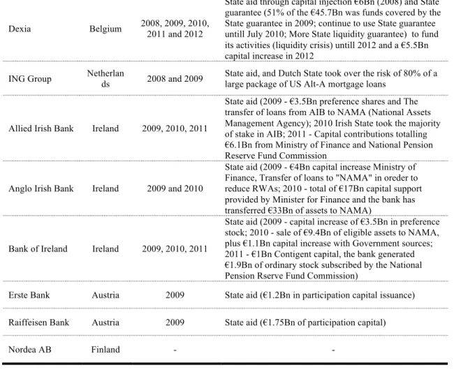
In Portugal, the main source of financial state intervention occurred in 2012 through hybrid instruments (CoCo’s – Contingent Convertibles, a security similar to a convertible bond, that converts into capital in case the issuer is not able to repay the debt; this instrument is accountable to Core Tier I capital) and the total help accounted approximately to €4.5B (taking into account the analyzed banks). The state intervention that occurred in France was a precautionary program, to avoid credit crunch. The three analyzed banks (BNP Paribas, Credit Agricole and Societé Générale) incurred in a state aid program that consisted on around €11B of subordinated hybrid government bonds. In Italy, the state intervention on banks occurred mainly in 2009 through convertible bonds (called the “Tremonti Bonds”). The German state intervention program affected one (Commerzbank) of the two analyzed banks (Deutsche Bank and Commerzbank), which incurred on a silent participation by the Special Fund for Financial Market Stabilization. One of the most critical analyzed markets was the Greek one, in which all the analyzed banks were intervened through direct capital injections (preference shares) and through convertible bonds. Greek banks and Greek economy were extremely affected not only by the international economic environment and banks performance during the sample period, but mostly due to Greek sovereign debt default (2012), which increased substantially banks’ losses through impairments. The banking crisis in Belgium affected both analyzed banks (KBC Group and Dexia). However, the intervention level on Dexia was much higher with several programs occurring between 2008 and 2012, consisting not only in capital injections (2008), but also in state funding guarantees. In the Netherlands, the ING Group (the only bank considered in the

sample) was subject to a state capital injection in 2008 due to bank’s bad performance and the bank need for capital in the considered year, and in 2009 the Dutch state took over the risk of 80% of a large package of US Alt-A mortgage loans, reducing ING’s Risk Weighted Assets (RWAs) and therefore improving solvency levels. Another financial market which was considered to be deeply connected to the US market was the Irish one. Its banks’ performance was highly affected in 2009 (right after the US financial turmoil), incurring on deep restructuring programs, which consequently affected the Irish State itself. Regarding the Austrian banks, Raiffeisen Bank and Erste Bank incurred on state capital injections of almost €3B during 2009, the most distressed period in the sample.

A deeper analysis on the bank default information is presented in the Appendix section on table VI.

Considering this information on bank defaults (39 default events recorded), it is now possible to choose the financial and macroeconomic variables in order to build a model for predicting bank default probabilities.

3.1.2. Explanatory variables

The variables chosen as drivers for bank default cover capital (Total equity / Total assets), asset quality (loan impairments / Net loans), management quality (cost-to-income ratio), earnings or profitability (Return on Assets), liquidity (Liquid assets / Short-term funding), market discipline (Net interest income / Net income), growth (liabilities growth) and the macroeconomic factors which could be sub-divided into business cycle variables and macroeconomic prices.

In table I it is performed a simple comparison between the variables in a non-default situation and a non-default environment situation. Through the analysis of this table, one can conclude that the bank-related variables have different behavior on Non-default and default situations. The table shows that defaulted banks have lower capitalization, lower earnings, and lower liquid assets as percentage of total assets. The loan to deposits ratio (LTD ratio) also shows that defaulted banks tend to have higher LTD ratio and lower market discipline defined by the net interest income to net loans ratio. It is also shown that defaulted banks have lower asset quality (meaning higher loan impairments to net loans ratio), lower cost-to-income ratio, lower growth and higher wholesale funding to total liabilities ratio. The macroeconomic variables behavior is the expected one (lower GDP growth rate, lower inflation and lower sovereign bonds interest rates on averaged defaulted banks), except the balance of payments whose behavior seems to be the opposite one.

Nevertheless, a t-test is performed on the chosen variables to assess their individual significance level, which gives the statistical interpretation of rejecting or not the null hypothesis, i.e. the hypothesis of the difference between average defaulted and non-defaulted variables be equal to zero.

Table I

Defaulted variables t-test

Variables Non-default Default

Mean Median Mean Median Standard _deviation t-student Total Equity / Total

Assets 5,81% 5,76% 4,18% 3,97% 0,024 -4,30*** Loan impairments/ Net loans 0,43% 0,30% 1,57% 0,65% 0,015 4,79*** Cost-to-Income ratio 50,36% 58,20% 40,04% 55,21% 0,387 -1,66 Return On Equity 21,97% 9,51% 20,71% 1,45% 2,783 -0,03 Return On Assets 0,37% 0,48% -1,57% -0,06% 0,020 -6,05*** Liquid Assets / Short-term funding 61,36% 47,80% 61,52% 49,84% 0,492 0,02 Liquid Assets / Total Assets 31,94% 29,05% 31,53% 27,83% 0,139 -0,18 Net Interest Income

/ Net Loans 3,11% 2,98% 2,63% 2,39% 0,011 -2,78*** Loan to Deposits ratio 123,22% 100,43% 197,34% 127,53% 2,249 2,06* Liabilities growth 10,03% 5,89% -1,55% -2,40% 0,180 -4,02*** Asset growth 9,88% 6,06% -1,32% -1,94% 0,177 -3,95*** GDP growth 1,49% 1,70% -3,03% -3,10% 0,028 -9,95*** Inflation Rate 2,51% 2,30% 0,99% 1,00% 0,011 -8,37*** Government bonds interest rates 4,58% 4,26% 6,89% 4,42% 0,026 5,63*** Balance of Payments (million euros) -7 744 -11 519 -578 -4 118 44 627 1,00

Notes: *, **, *** denotes significance level at 10, 5 and 1 percent level, respectively.

Through the performed t-test, one can conclude that the difference between the average from the defaulted variables and the non-defaulted is significant within the following variables, considering a 5% significance level:

- Loan impairments / Net loans; - Return on Assets;

- Net interest income / Net loans; - Liabilities and Asset growth; - GDP growth rate;

- Inflation rate;

- Government bonds interest rates;

Thus, at a significance level of 5%, one can reject the hypothesis of the mentioned difference, between defaulted and non-defaulted variables, be insignificant (equal to zero), meaning that the observed difference between the sample mean and the average of the defaulted variable can be interpreted as the actual difference observed in table I.

In the following subsections the variables are discussed in more detail.

3.1.2.1. Capital

The variable used as measure of capital was the simple leverage ratio Total equity / Total assets. It is a simple unweighted leverage ratio, different from the regulatory capital to risk weighted assets ratio (CT1 ratio). The Basel regulatory capital framework has been changing across the sample period. Another reason why the simple leverage ratio is used to measure capitalization is the lack of coverage for the whole sample period and the complexity to compute the regulatory ratio. The analysis made in Kocagil, et al. (2002), suggests that total equity over total assets is an informative measure for capital. Most literature uses the simple leverage ratio due to similar limitations. Table I shows that the ratio is expected to have a negative

impact on the probabilities of default, which means that a higher ratio would lead us to lower probabilities of default, and higher ability to absorb shocks on bank performance.

In the figure 4 of the appendix section the evolution of the annual average for the capital ratio, in the studied sample, is illustrated. A decline is observed in the average of total equity to total assets ratio in 2008, the period in which we observed 5 defaults in our sample (shown in previous figure 2), and in 2009 (the most defaulted period) we observed an increase in the average ratio, which can be explained by the capitalization programs lead by the governments that occurred in the period (2009). In 2011 and 2012 we observe another decline in the ratio matching with another default period (9 observed defaults in 2012).

3.1.2.2. Asset Quality

To determine the asset quality of a financial institution, the considered indicator was the loan impairments to total net loans ratio. The variable measures loan losses as a percentage of total loans. Since the majority of the analyzed banks are commercial banks and their core business is loans and advances to clients, the ratio loan impairments to total net loans can be seen as a good measure for asset quality. The evolution of the variable shows the great increase on the defaulted periods, suggesting a positive impact on probabilities of default of a financial institution (figure 5 – Appendix section), in which a higher ratio would imply higher probabilities of a bank default.

3.1.2.3. Management

The management quality of a financial institution could be an important driver of a bank default. The cost-to-income ratio is used to determine the management quality, which can be viewed as a measure of efficiency, since it measures the operating costs as percentage of the banking income. A higher ratio would imply lower efficiency as such it is reasonable to expect a positive impact on the probabilities of default (higher ratio would mean higher probabilities of default). The pattern observed in figure 6 (Appendix section) shows that there is an increase in the 2008’s cost-to-income ratio, followed by a decrease in 2009 and then an increase in the average of 2012. The pattern in 2009 could be also explained by the severe restructuring programs several banks adopted, to face high losses.

3.1.2.4. Earnings

The standard variables Return on Equity and Return on Assets (after-tax) are used to capture bank earnings. It is expected that a bank with higher returns should be more capable of absorbing external shocks, however we should take into consideration the fact that those external shocks would majorly affect bank returns. Consequently, an affected financial institution would present lower returns and lower ratio, these external shocks can express through losses due to operational risk such as results of financial operations or impairments (a company's asset that is worth less on the market than the value listed on the company's balance sheet). The financial crisis was tremendous and some of the analyzed institutions were unable to absorb the external shocks and recorded negative equity, which affected the computation of the

was the return on assets ratio, which proved to be consistent in situations of distress such as negative equity, as it is observable in figure 8 (Appendix section).

3.1.2.5. Liquidity

Liquidity measures the ability of the assets convertibility into cash. Liquid assets are those that can be converted into cash quickly if needed to meet financial obligations; examples of liquid assets generally include cash, central bank reserves, government debt (which is easily converted through secondary markets) or loans ad receivables to banks (short-term). To remain viable, a financial institution must have enough liquid assets to meet its short-term obligations, such as withdrawals by depositors2. In order to measure for liquidity we considered three possible variables, the liquid assets to total assets, which measures the percentage of liquid assets in the whole financial institution; and the liquid assets to short-term funding, which is similar to a liquidity coverage ratio. The objective of the Liquidity Coverage Ratio is to promote resilience to liquidity risk in a short-term basis. The official (Basel III) Liquidity Coverage Ratio provides information about the stock of liquid assets that could be converted into cash in private markets in order to meet the bank needs for a 30 calendar day stress scenario. The assessed indicator is a simplified version of the official liquidity coverage ratio and tries to capture the capacity of converting assets into cash in order to meet financial obligations (measured by short-term funding, which includes deposits from other credit institutions and deposits from customers). Figures 9 and 10 (of Appendix section) show the average evolution of the considered variables. The observed trend shows a decrease in the average liquid assets between                                                                                                                

2008 and 2009 followed by an increase in the upcoming years. In the financial crisis (especially in 2008 and 2009) one can observe a liquidity short-fall, which should be expected. It is expectable that higher ratios would improve the solvency level of the financial institution and therefore decrease the probability of default (negative impact on probability of default).

Since liquidity risk is a very important issue on credit institutions, another commonly used variable for assessing a bank’s liquidity that should be tested is the loan to deposit ratio (LTD ratio). A higher ratio could mean that the bank might not have enough liquidity to face unforeseen fund requirements. Hence, it is expected a positive impact on probabilities of default, which means that a higher ratio would imply higher probabilities of default. However, if the ratio is too low, the bank may not be earning as much as it could be. The European recommendation for this ratio is around 120% on loans to deposits ratio. Figure 11 (of Appendix section) shows the evolution of the average ratio across the period.

3.1.2.6. Market Discipline

The search for market share might encourage financial institutions to increase deposit rates and decrease loan interest rates jeopardizing solvency levels. However, these financial institutions, by increasing deposit rates or decreasing loan interest rates, may not be proceeding in a sustainable manner, and so proceeding with lack of market discipline (Poghosyan & Cihak, 2011). The variable chosen to measure market discipline was the ratio net interest income to net loans, which captures the gap between the interest volume, majorly (considering that the analyzed institutions are commercial banks) on credit and the interest expense, majorly on deposits, as

percentage of total loans of the analyzed bank. Capturing discipline both in credit (revenues) and in deposits (expenses). Consequently, it is expected that a higher ratio would imply lower probabilities of default (a negative impact on probabilities of default). The trend of the average ratio is observable in figure 12.

3.1.2.7. Growth

The growth rate of a financial institution, in general, should suggest that a bank with exceptional or excessive growth has experienced problems because its management or structure was not able to sustain such unusual growth (Kocagil, Reyngold, Stein, & Ibarra, 2002). Therefore, the growth could be a good indicator in order to account for the unsustainability of the specific banking business. The variable chosen to measure the growth rate of a specific financial institution is the liabilities growth rate. In Kocagil, et al. (2002), the variable is compared to other potential indicators for measuring growth and it seems to be the most accurate indicator, it should be noticeble that the banking business is highly leveraged and so, liabilties growth should provide a good insight on this scope. The recent financial crisis brought to us a considerable number of bank restruturing programs, which, in most cases, resulted in downsizing of their balance sheets. Taking into account these factors, it is expected that this indicator should impact positively on the probabilities of default, meaning that higher liabilities growth rates should imply higher probabilities of a distress situation. However, these undergoing restructuring processes can affect the modeling analysis. Figure 13 (of Appendix section) presents the average growth rate of liaibilities during the considered period.

3.1.2.8. Macroeconomic environment factors

The financial crisis we still live on has been a good reminder of how the real economy impacts banking performance. The losses incurred on the banking sector in the beginning of the financial crisis destabilized the banking sector and triggered a vicious cycle. Problems in the financial system can lead to a downturn in the real economy, which in turn hits back banking performance (Bank for International Settlements, 2010). Considering the impact of the macroeconomic environment on the financial sector is an important issue in prudential modeling; this study also provides some insight on this subject. In order to capture the macroeconomic environment impact on banking performance two sets of macroeconomic variables are considered, one measuring the business cycle impact, the other measuring the macroeconomic prices. For the business cycle, the variable chosen was the Gross Domestic Product (GDP) growth rate, which captures accurately the business cycle, reflecting the upward and downward movements of the economic activity. The impact on the probabilities of default should be negative, meaning that an increase in the GDP growth rate should decrease the probability of default of a credit institution (ceteris paribus) – the average behavior of GDP growth rate is presented in figure 14 (of Appendix section).

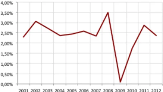
For the macroeconomic prices, there are several indicators that could be considered in order to capture different scopes of macroeconomic prices. Inflation is an important measure for the price level of goods and services in an economy and could influence the bank performance. Considering the historically stable and low levels of inflation in the Euro area (the analyzed region) we should take precautions on the expectations of its impact on probabilities of default. The behavior of inflation

rates in the Euro area countries (presented in figure 15 of Appendix section, as the year average) shows a low level across the period and in some cases deflation is observable. Hence, expectations should take into consideration how deflation (decrease in the general price level of goods and services) or disinflation (decrease in the rate of inflation) could impact banking performance. Usually, a decline in expected inflation will lead to a decline in the nominal interest rate. However, once the nominal interest rates are set to close to zero (situation similar to Euro area’s), a decline in the expected inflation will cause the real interest rate to rise (since it is not possible to decrease the interest rate). This behavior is likely to slow down the economic activity through an increase in the cost of capital and discouraging borrowing among consumers and enterprises. Another way deflation could impact banking activity is through the value of debt. Deflation increases the real value of debt while decreasing the value of collateral for loans. The combination of these factors could sharply increase the loan losses and affect bank performance3. The figure above illustrates the evolution of inflation in Euro area, and it is observable the mentioned low levels and a sharp decline in 2009. Therefore, it should be expected that inflation rate impacts negatively on probabilities of default, which means that a decrease in inflation would increase the probabilities of a bank default. If inflation recorded higher average levels, the expected results on the prediction model could be inverted, in the sense that in economies with high inflation rates, credit institutions will lend less, the financial markets will be smaller, less liquid and facing higher volatilities impacting negatively in the long-run the bank performance (Boyd, Levine, Smith, & D., 2000).

Another tested variable that fits in macroeconomic prices category is the sovereign bonds interest rates. This variable can be interpreted as the sovereign risk, which could have impact on banks, in the sense that banks own large sovereign bonds portfolios. However, the sovereign bonds yields’ impact could be dubious since higher yields imply more risk and in some cases (such as Greek sovereign bonds) losses due to sovereign default, but in other sense, higher yields means not only higher risk but also higher interest earnings and so higher financial margin implying better banking performance. Taking this dual effect on banking performance, it is difficult to create expectations on sovereign bond interest rates. The sovereign risk affects financial institutions in a more systemic way and could have a contagion effect on the whole financial system. Figure 16 illustrates the average Euro area sovereign bond yields evolution through the considered period.

Furthermore, another macroeconomic environment variable, the country’s balance of payments, was also tested in the prediction model. The rationale behind this indicator is that it gives an insight on the level of debt or surplus of the whole economy where the bank is based in. If an economy is highly indebted it means that financial institutions should fund themselves with foreign funding sources through financial markets and less funding from deposits from customers, this fact would make the financial institution more vulnerable to money markets, which bears more volatility to the funding structure. The fact that households and corporates are highly indebted could make them more vulnerable to external shocks (such as unemployment situations or slowdowns in business activity). This fact could have tremendous repercussions on the banking performance, with great income losses. Hence, it is expected that a higher balance of payments indicator (surplus) should impact negatively on the probabilities of default, i.e. a higher deficit on balance of payments

would be associated with a higher probability of default of a bank based in the respective country. The average Euro area balance of payments evolution is presented in figure 17 (of Appendix section).

Figure 17 shows the tremendous adjustment that has been occurred in the Euro area countries after the 2008 crisis. This fact can contribute to a more difficult analysis in terms of the variable impact on banking performance.

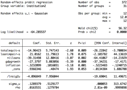
4. RESULTS AND DISCUSSION

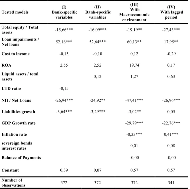
In order to analyze possible drivers of bank default, several probit regression models with random effects were tested, presented in the table below. The default indicator is used as dependent variable, which is already explained in the data description section (section 3.1). The default variable takes value 1 if the analyzed bank incurred in default in a given period (this means that the bank needed financial support to keep their activities or financial guarantees – from its respective State - in order to fund their activities) or 0 otherwise. The following table presents the most relevant estimation results.

Table II

Panel Data Probit Estmation Results

Tested models (I) Bank-specific variables (II) Bank-specific variables (III) With Macroeconomic environment (IV) With lagged period Total equity / Total

assets -15,66*** -16,09*** -19,19** -27,43***

Loan impairments /

Net loans 52,16*** 52,64*** 60,13** 17,95**

Cost to income -0,15 -0,10 0,12 -0,29

ROA 2,55 2,52 19,74 0,17

Liquid assets / total

assets 0,12 1,27 0,63

LTD ratio -0,15

NII / Net Loans -26,94*** -24,92** -47,41*** -26,96***

Liabilities growth -3,64*** -3,29*** -3,02** 0,05 GDP Growth rate -29,79*** -22,76*** Inflation rate -0,33*** 0,41*** sovereign bonds interest rates 0,01 0,08 Balance of Payments -0,00 -0,00 Constant 0,39 0,07 0,57 0,57 Number of observations 372 372 372 341

Notes: *, **, *** denotes significance level at 10, 5 and 1 percent level, respectively.

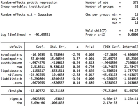
In the first regression model, the drivers used to explain default were bank-specific financial indicators only. Following a criterion already mentioned above, first the determinants related with Capital, Asset quality, Managerial skills, Earnings, Liquidity, Market discipline and Growth are incorporated. Capitalization was measured by ratio of total equity over total assets, higher ratio means the institution is better prepared to absorb external shocks. The ratio of loan impairments over net

loans is used to measure asset quality (from Profit & Loss account), where one could expect that a higher ratio would imply a higher probability of default. For managerial skills the ratio used was the cost-to-income, which one would expect a higher ratio for higher probabilities of default, meaning a higher percentage of costs in terms of total income implying less efficient management skills. The return on equity and return on assets ratios are used to measure the bank earnings, with higher ratios suggesting better earnings and so lower probabilities of default. Liquidity is measured in different ways, by liquid assets (given by central bank and other credit institutions claims, cash reserves and trading assets) over total assets, through total assets over deposits and short-term funding and through the loan to deposits ratio, their rationale was already approached in the subsection 3.1.3.5. Liquidity. Market discipline is measured by the ratio net interest income over net loans, a lower ratio would mean the institution has a more aggressive strategy in order to gain market share, both in credit conceded to customers and in deposits from customers but it could imply lower risk perception, meaning a higher probability of default.

Taking into account the first two panel data probit regression models with random-effects that consider only bank-specific financial indicators, their results suggest that the impact of capital ratio on probabilities of default is significant (at 1% significance level) and in line with the expected results namely a higher capital ratio would imply a lower probability of default. With the opposite sign, but also significant (significance level of 1%), the ratio for asset quality suggests a behavior similar to the expected, namely a higher ratio of loan impairments to net loans means a higher probability of default. The results on managerial skills, measured by the cost-to-income ratio, suggest that the variable is not relevant; this may be explained by most banks incurred in restructuration programs, which consisted on huge cost

reductions and even in size reductions (balance sheet size reductions). The ROA (Return on Assets) variable resulted not to be statistically significant. The chosen variables for liquidity showed no statistically significant results, the three variables liquid assets as percentage of total assets, liquid assets to short-term funding and the loan to deposits ratio. Liquidity risk should have two pillars, the idiosyncratic pillar which should be captured by the analysis of the quality of their liquidity risk management, and the systemic pillar, which impacts on every credit institution of the market (such as severe liquidity disruption in the market). Wu & Han (2013) suggest that systemic liquidity risk was the major determinant for the recent bank failures (2008 and 2009). This could explain the statistical insignificance of the idiosyncratic liquidity risk presented in these predictions. Another statistically significant (with a 5% significance level) variable in the first two considered estimation outputs was the one related with market discipline (Net interest income over net loans) and it is in line with the expected results. Suggesting that higher financial margin over loans (lower aggressiveness in the market) implies lower probability of default (negative impact on probability of default). The measure for growth (liabilities growth rate across the sample period) does not behave as it was expected. Its impact on default probabilities is negative, which means that a higher growth rate of liabilities would imply lower probabilities of default. This behavior could be described with a similar rationale as of the variable referring to managerial skills (cost to income ratio), with big restructuring programs taking place in the majority (non defaulted and specially defaulted) of banks. However, the behavior presented in the figure 12 (section 3.1.3.7.) indicates that there was exceptional growth in the periods prior to the financial crisis (2008), suggesting that further analysis on lagged indicator could be useful in the study of this variable, however, such analysis was not performed due to database constraints.

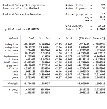
In the third output regression model the selected macroeconomic variables (GDP growth, Inflation rate, 10 year government bonds interest rates and the Balance of payments) were added to the previous estimations. These macroeconomic variables refer to the country in which the financial institution is based on. The results of this third estimation model demonstrate that macroeconomic environment is highly connected with banking activities, which is in compliance with the expected outcomes. The results suggest good significance levels for GDP growth rate and for inflation rate, with significance levels below 1%. In terms of GDP growth rate, the results imply a negative relation between the GDP growth and the default probabilities of banks; a higher GDP growth rate would imply a lower probability of default. This is in line with the expected result and with the theory that states that business cycles affect banking performance. The other relevant variable was inflation rate, impacting on the same direction as the GDP growth rate variable, with higher inflation rates implying lower levels of default probability. Deflation or disinflation could be caused (more likely) by a sharp decline in credit supply or a contraction in the economy. These deflation periods or really low levels of inflation could have impacted negatively on the banking industry, by increasing the real value of debt (of households and corporates), since the nominal value of the debts remains constant and prices decline, while decreasing the value of collateral for loans, impacting negatively on banks’ earnings. Another contribution to the negative impact of inflation in banking performance, already approached in section 3.1.3.8, could be through interest rates behavior. A decline in expected inflation will lead to a decrease in the nominal interest rate. However, once the nominal interest rates are close to zero (situation similar to Euro area’s), a decline in the expected inflation will cause the real interest rate to rise (since it is not possible to decrease the interest rate). This behavior is likely

to slow down the economic activity through an increase in the cost of capital and discouraging borrowing among consumers and corporates, affecting banking performance. The other macroeconomic considered variables (sovereign bonds interest rates and balance of payments) have no sufficient significant level in order to be properly interpreted. Regarding the bank related financial variables the results suggest similar trends and significance levels (slight increase) comparing with the previous regression model.

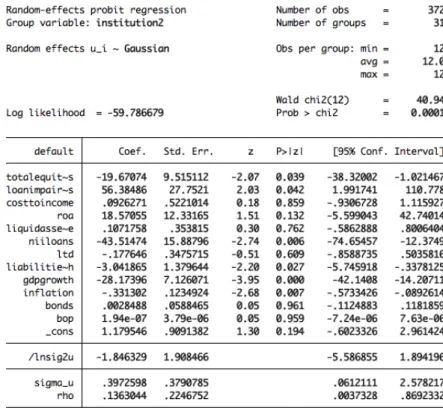
Another relevant performed regression model was a lagged (by one period) estimation. This regression model exhibits no different trends in the studied variables. The only significant change was in liabilities growth rate variable, which loses its significance level. This adjustment could suggest a change in behavior when this variable is analyzed in a lagged approach.

5. CONCLUSION

This study approaches the main impacts on bank default through a new database, which considers annual financial reports provided by the banks. This fact can bring some limitations on the analysis due to misreporting or creative accounting. The geographical perimeter of this study was the Euro area of which there is less research, since did not exist many relevant bank distress situations until the recent crisis.

The performed estimations give good insight on the behavior of both financial and macroeconomic variables regarding distress situations of financial institutions. Specially, measures for capitalization, asset quality, market discipline, GDP growth

the other hand variables measuring efficiency, earnings, liquidity and other tested macroeconomic indicators (such as government bonds interest rates and balance of payments) did not appear to be relevant on the evaluation of bank distress situations. Another indicator that could improve risk assessment is the measure for growth (liabilities growth rate), however this variable should be tested using different approach, such as a lagged variable (and possibly by more than one period). This variable could provide an insight on unsustainable growth, which could reflect its impact with certain delay.

The recent financial crisis has raised important issues in terms of banking supervision. Significant steps have been taken regarding the required levels of capital (which is in line with the estimation done in this study), however other measures could be done, such as the adoption of countercyclical approaches (for example countercyclical buffer on capital requirements) providing a combined evaluation of both financial and macroeconomic (business cycles) environment. Asset quality evaluation and market discipline shall not be forgotten; restrictive measures on deposits (limits to its interest rates, in order to keep discipline on the market) have been carried out in some countries, similar measures on loans could be subject of further analysis. Inflation rates should also be considered in prudential analysis, not only when it increases to high levels but also when it declines to particularly low levels due to its negative impact on economic development and on financial system.

This study suggests future research that can bring value to banking supervision and to society in general, namely in the development of the banking union that is taking place within the Monetary Union.

Given this framework, one can conclude that both bank-specific and macroeconomic variables affect bank performance and therefore the solvency levels

of a financial institution. Thus, supervisory authorities should take in consideration not only the financial specific performance but also the macroeconomic environment where the financial institution is based on (specially the business cycles and macroeconomic prices).

REFERENCES

Ahangarani, P. M. (2007). A New Structural Approach to the Default Risk of Companies. University of Southern California iversity of Southern California, Economics Department . Antunes, A., & Silva, N. (2010). An Application of Contingent Claim Analysis to the Portuguese Banking System . Bank of Portugal , Financial Stability Report.

Bank for International Settlements. (2010). Countercyclical capital buffer proposal. Basel Comittee on Banking Supervision .

Black, F., & Cox, J. C. (1976). Valuing Corporate Securities: Some Effects of Bond Indenture Provisions. Journal of Finance .

Boyd, J. H., Levine, R., Smith, & D., B. (2000). The Impact of Inflation on Financial Sector Performance.

Bordo, M. D., & Landon-Lane, J. S. (2010). The Global Financial Crisis of 2007-08: Is It Unprecedented?

Curry, T. J., Elmer, P. J., & Fissel, G. S. (2003). Using Market Information to Help Identify Distressed Institutions: A Regulatory Perspective. FDIC Banking Review , 15.

DG Competition - European Commission. (2013). Aid in the context of the financial and economic crisis.

http://ec.europa.eu/competition/state_aid/scoreboard/financial_economic_crisis_aid_en.html Federal Reserve. (2014). What is the difference between a bank’s liquidity and its capital? http://www.federalreserve.gov/faqs/cat_21427.htm .

FDIC. (2003). How Real is the Threat of Deflation to the Banking Industry? https://www.fdic.gov/bank/analytical/fyi/2003/022703fyi.html .

Geske, R. (1977). The Valuation of Corporate Liabilities as Compound Options. Journal of Finance .

Hong, H., & Wu, D. (2013, October). Systemic Funding Liquidity Risk and Bank Failures. Kocagil, A. E., Reyngold, A., Stein, R. M., & Ibarra, E. (2002, July). Moody’s RiskCalc™ Model for Privately-Held U.S. Banks.

Merton, R. C. (1974). On the Pricing of Corporation Debt: The Risk Structure of Interest Rates. Journal of Finance , 29, 449-70.

Poghosyan, T., & Cihak, M. (2011). Determinants of Bank Distress in Europe: Evidence from a New Data Set. Springer Science .

Porath, D. (2006). Estimating Probabilities of Default for German Saving Banks and Credit Cooperatives.

Thomson, J. B. (1991). Predicting Bank Failures in the 1980s. Federal Reserve Bank of Cleveland, Economic Review .

APPENDIX

Appendix data description

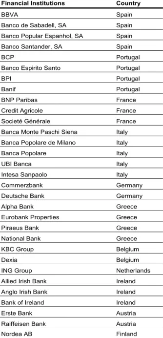
Table III

List of Financial Institutions Considered in the Sample

Financial Institutions Country

BBVA Spain

Banco de Sabadell, SA Spain Banco Popular Espanhol, SA Spain Banco Santander, SA Spain

BCP Portugal

Banco Espirito Santo Portugal

BPI Portugal

Banif Portugal

BNP Paribas France

Credit Agricole France Societé Générale France Banca Monte Paschi Siena Italy Banca Popolare de Milano Italy Banca Popolare Italy

UBI Banca Italy

Intesa Sanpaolo Italy

Commerzbank Germany

Deutsche Bank Germany

Alpha Bank Greece

Eurobank Properties Greece Piraeus Bank Greece National Bank Greece

KBC Group Belgium

Dexia Belgium

ING Group Netherlands Allied Irish Bank Ireland Anglo Irish Bank Ireland Bank of Ireland Ireland

Erste Bank Austria

Raiffeisen Bank Austria

Table IV

Bank-specific variables by category

Variables Category

Total Equity / Total Assets Capital

Loan impairments/ Net loans Asset quality

Cost-to-Income ratio Management

Return On Equity Earnings

Return On Assets Earnings

Liquid Assets / Short-term funding Liquidity

Liquid Assets / Total Assets Liquidity

Loan to Deposits ratio Liquidity

Net Interest Income / Net Loans Market discipline

Default Characterization

Figure 2 - Number of Defaults, by Year

Table V

Default situations by bank and period

Financial

Institutions Country Default Notes

BBVA Spain - - Banco de Sabadell, SA Spain - - Banco Popular Espanhol, SA Spain - - Banco Santander, SA Spain - -

BCP Portugal 2012 State aid through Contingent Convertibles (€3Bn) Banco Espirito

Santo Portugal - -

BPI Portugal 2012 State aid through Contingent Convertibles Banif Portugal 2012 State aid through capital injection and Contingent _{Convertibles (€1.1Bn)} BNP Paribas France 2009 State aid to avoid credit crunch in french economy _{€5.1Bn Subordinated government bonds} Credit Agricole France 2008 State aid to avoid credit crunch in french economy €3Bn _{Subordinated government bonds} Societé Générale France 2009 State aid to avoid credit crunch in french economy Banca Monte

Paschi Siena Italy 2009 and 2012

State aid through Tremonti bonds €1.9Bn in 2009, €3.9Bn hybrid instruments ("Monti Bonds") 2012 Banca Popolare

de Milano Italy 2009 State aid through "Tremonti Bonds" (€500M) Banca Popolare Italy 2009 State aid through "Tremonti Bonds" (€1.45Bn) UBI Banca Italy - -

Intesa Sanpaolo Italy - -

Commerzbank Germany 2008 and 2009 State aid through Special Fund for Financial Market _{Stabilization (SoFFin)} Deutsche Bank Germany - -

Alpha Bank Greece 2009 and 2012 State aid capital injection through preference share _{€940M (2009) and €2.9Bn convertible bonds (2012)} Eurobank

Properties Greece 2009 and 2012

State aid through preference share €950M (2009) and €3.1Bn Bonds (2012)

Piraeus Bank Greece 2009 and 2012 State aid through preference share €370M (2009) and €7.3Bn through Share capital increase Contigent convertible securities (2012)

National Bank Greece 2009 and 2012 State aid through preference share (2009) and Bonds ₍₂₀₁₂₎ KBC Group Belgium 2008 and 2009 State aid €7Bn in perpetual , non-transferable, non-voting core-capital securities €3.5Bn each year (2008 and