Revista Brasileira de Agricultura Irrigada v.9, nº.4, p. 225 - 231, 2015 ISSN 1982-7679 (On-line)
Fortaleza, CE, INOVAGRI – http://www.inovagri.org.br DOI: 10.7127/rbai.v9n400305
Protocolo 305.15 – 23/05/2015 Aprovado em 03/07/2015
AN EMPIRIC MODEL FOR PREDICTING SOIL DAILY EVAPORATIONS: SOIL AND ATMOSPHERIC VARIABLES
I. M. Ponciano1, J. H. Miranda2, M. A. Santos1, Q. de Jong van Lier3, V. F. Grah4 ABSTRACT
The evaporation of soil water (Es) affects water availability for crop transpiration which is directly related to crop growth and yield. Principles of the evaporation process are well known, but evaporation prediction using a simple model is more difficult. We propose a simple empirical one-day step model to estimate Es based on soil water content and potential evaporation (E0). An experiment was performed by carefully accommodating a sandy-clay soil in 14 drainage lysimeters of 0.5 m3 in each of which two TDR probes were installed at 0.05 m depth for water content measurement. The soil in the lysimeter was gradually saturated using an auxiliary water column connected to the drainage outlet. Evaporation was measured by the daily reading of the variation of the water level inside the column. Class A pan evaporation was used to assess the daily E0. The relationship among Es/E0 and the initial soil moisture were used to develop and test the model. The statistical results (R² 0.82 and error 0.07%) over a wide range of water contents (0.28 to 0.47 m3m-3) suggest the proposed model to allow a good estimation of soil water evaporation.
Keywords: soil evaporation, time domain reflectometer, class A pan, lysimeter
UM MODELO EMPÍRICO PARA ESTIMATIVA DA EVAPORAÇÃO DIÁRIA DO SOLO: VARIÁVEIS DO SOLO E ATMOSFÉRICA
RESUMO
A evaporação da água do solo (Es) afeta a disponibilidade de água para a transpiração da cultura que está diretamente relacionada com o crescimento e a produtividade das plantas. Princípios do processo evaporativo são bem conhecidos, mas a predição da evaporação por um modelo simples é mais difícil. Propõe-se um modelo empírico diário simples para estimar
1
PhD fellow, Luiz de Queiroz College of Agriculture, University of São Paulo ESALQ/USP, Piracicaba – São Paulo. e-mail: [email protected]; [email protected].
2
Associate professor, Luiz de Queiroz College of Agriculture, University of São Paulo ESALQ/USP, Piracicaba – São Paulo. e-mail: [email protected].
3
Full professor, Center for Nuclear Energy in Agriculture, University of São Paulo CENA/USP. e-mail: [email protected].
4
Professor, Federal Institute of Education, Science and Technology Goiano IFGoiano. e-mail: [email protected].
Es com base no conteúdo de água do solo e evapotranspiração potencial (E0). Um experimento foi cuidadosamente conduzido, acomodando um solo areno-argilosos em 14 lisímetros de drenagem de 0,5 m3 em cada uma das quais duas sondas foram instaladas na profundidade de 0,05 m para a medição do teor de água. O solo do lisímetro foi gradualmente saturado utilizando uma coluna de água auxiliar ligado à saída de drenagem. A evaporação foi medida pela leitura diária da variação do nível da água no interior da coluna. Tanque de evaporação Classe A foi usado para avaliar a E0 diária. A relação entre Es/E0 e da umidade inicial do solo foram usados para desenvolver e testar o modelo. Os resultados estatísticos (R² 0,82 e erro de 0,07%) correspondente a uma ampla variação do conteúdo de água (0,28-0,47 m3m-3) sugerem que o modelo proposto possibilita uma boa estimativa da evaporação da água do solo.
Palavras-chave: evaporação do solo, reflectometria no domínio do tempo, tanque classe A, lisímetro
INTRODUCTION
The prediction of soil evaporation (Es) is essential for any soil water balance study. It is an important variable in irrigation water management, especially for reducing the available soil water for transpiration. It may also enhance the salinization processes by promoting transport of salts to the surface layer, particularly in arid and semi-arid regions. Generally, ES represents 10% of evapotranspiration (CAMPBELL, 1985), being more important under sparse vegetation, especially in dryland ecosystems where it can accounts for 30 to 90% of evapotranspiration (STROOSNIJDER, 1987; BALWINDER-SINGH et al., 2014). Considering sustainable water application, evaporation is regarded as a non-beneficial loss. Although there are several models available to estimate soil evaporation, an important challenge in irrigation management is to establish a robust model requiring easily available data.
There is a vast number of approaches to describe soil evaporation, however the one presented by Ritchie (1972), based on the concept of Philip (1957), has been extensively used and incorporated into soil-plant-atmosphere models such as DSSAT and APSIM series (BALWINDER-SINGH et al., 2014), FAO AguaCrop (RAES et al., 2009; VANUYTRECHT et al., 2014), SWAP (KROES et al., 2008) and HYDRUS (SIMUNEK et al., 2005). When soil water content is high, evaporation rate is relatively
constant and supported by internal capillary flow (YIOTIS et al., 2006). In this stage, Es is determined by the amount of radiant energy received at the soil surface and the air drying potential and lasts until a generic volume of water is evaporated (RITCHIE, 1972). When soil becomes drier, the evaporation rate gradually drops because of a transition to diffusion-limited vapor transport (OR et al., 2012). In this second stage the evaporation rate only depends on soil hydraulic properties and the evaporative rate attenuation is a function of the square root of time (HILLEL, 1980; MONTEITH, 1981). Campbell (1985) suggests a third stage in which the evaporation rate is very low (residual evaporative rate).
This approach has been applied over different ecosystems showing a good fit of evaporation rates to mini-lysimeter measurements (METZGER et al., 2014; PAREDES et al., 2015; WEI et al., 2015). Nevertheless, more robust studies indicate that Es during the second stage is not solely dependent on soil hydraulic properties, but also on atmospheric evaporative demand (JOHN, 1982; BALWINDER-SINGH et al., 2014). Furthermore, Wallace et al. (1999) found that, despite the ability to providing good estimates of cumulative soil evaporation over large periods (weeks or months), the model was unable to achieve good results on the daily scale.
In order to contribute to the prediction of evaporation we aimed to propose a new empirical daily model considering the three
VARIABLES
evaporative stages based on commonly measured quantities: the 0.05 cm depth soil water content and the class A pan evaporation.
MATERIALS AND METHODS The empirical model
An empirical model for the prediction of soil evaporation rate (Es, mm d-1) was formulated that considers the Campbell evaporation rate curve:
2 s i 0 s ln b a E E (1)
where E0 is the potential evaporation (mm d-1), θi is the daily early morning (initial) soil water content (m3 m-3), θs is the saturated soil water content (m3 m-3), and a and b are empirical parameters (-). Notice that, according to this equation, for values of θi close to θs, that correspond to near saturation conditions, Es tends to a constant value of 1/a (first stage). As
θi reduces, Es diminishes (second stage of soil evaporation). Finally, when θi tends to zero, Esoil also tends to zero.
Experimental setup
An experiment was conducted in a greenhouse at the University of São Paulo in Piracicaba (SP), Brazil. 14 lysimeters (volume 0.5 m³, height 0.60 m and upper diameter 1.1 m) were installed in a regular spacing at 0.15 m above the ground. A drainage system was connected composed of two layers of geotextile material (diver-geofort gf07 1.15 m) separating the soil material from an underlying 0.15 m layer of gravel, connected at the bottom to a drainage outlet.
The soil material was of sandy texture (13% clay, 9% silt and 78% sand) and was carefully accommodated in the lysimeters. Initially, the lysimeters were filled to the top establishing a density of 1.4 g m-3. 28 TDR probes (3 rods, 0.10 m long, 0.03 m root diameter, 0.17 m spaced) were installed at 0.05 m depth (two probes per lysimeter) to the estimate soil water contents (θ) from the dielectric permittivity (Ka) by
3 5 2 Ka 10 6953 . 2 Ka 0016 . 0 Ka 0395 . 0 0146 . 0 R² = 0.9923 (2)
A copper-constantan thermocouple was installed at 0.05 m depth in each lysimeter to monitor the soil temperature.
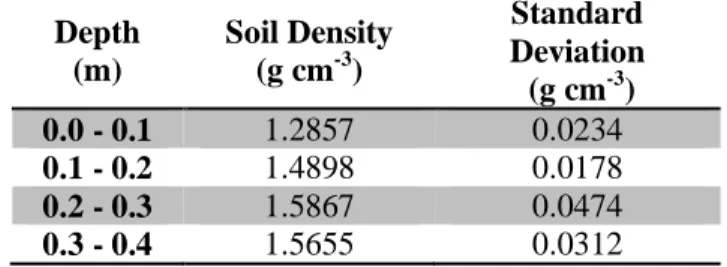
The soil material in the lysimeters was gradually saturated by capillarity with 0.3 dS m-1 water in a 3 days process using an auxiliary water column connected to the drainage outlet. Complete saturation was identified when the soil surface showed signs of saturation. The drainage outlet was then removed and the lysimeter returned to the free drainage condition. This procedure was repeated twice. A descent of the soil surface of about 0.10 m (± 0.04 standard deviation) was observed by the end of the process, when the soil bulk density was determined for each depth (Table 1).
Table 1. Final soil bulk density (average and standard deviation) per depth in the lysimeters
Depth (m) Soil Density (g cm-3) Standard Deviation (g cm-3) 0.0 - 0.1 1.2857 0.0234 0.1 - 0.2 1.4898 0.0178 0.2 - 0.3 1.5867 0.0474 0.3 - 0.4 1.5655 0.0312
The saturation-drainage procedure described above was performed to allow for a natural consolidation and leaching (ZAREI et al., 2010).
Similar to common practice in irrigated areas, Class A pan evaporation (E0) was measured inside the greenhouse in the centre of the greenhouse at 1.5 meter from the nearest lysimeter.
Evaporation rate and monitoring of variables
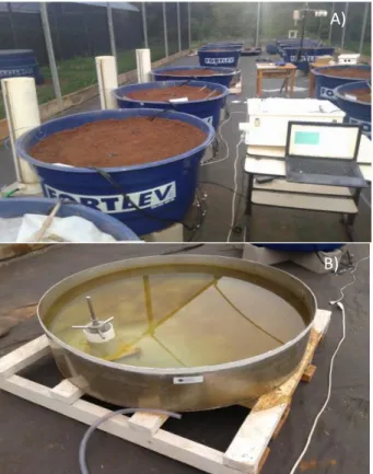
The soil evaporation rate (Es, mm d-1) was determined from the daily readings of the variation of the height of the auxiliary water column. Initially the water level inside the lysimeter was at about 1/3 of the top. At the morning of the first day, the soil water content at 0.05 m depth, the water level of the Class A pan and the water level readings of the auxiliary column were recorded (Figure 1).
Figure 1. Experimental setup to measure surface
(0.05 m) dielectric permittivity (Ka) using TDR, lysimeter and auxiliary column used to monitor the water level inside the lysimeters (A); Class A pan used to measure atmospheric demand (B)
After that, the auxiliary column was covered to stop its evaporation. At the second
day, the procedure was repeated. From these observations Es (mm d-1), E0 (mm d-1) and the daily initial water content θinitial were calculated. These quantities were used to calibrate the empirical model at daily scale.
Willmott’s index of agreement (d), the coefficient of efficiency (E) by Nash and Sutcliffe (1970), and the root mean square error of prediction (RMSEP) were used for model evaluation.
RESULTS AND DISCUSSION
The model fit to experimental data is shown in Figure 2. The value of parameter a was 1.4961 indicating that stage 1 evaporation is 0.67 (1/1.4961) or 67% of potential evaporation. A 100% match would have been expected, indicating that there is a difference in aerodynamic resistance between the lysimeters and the class A pan, possibly because of the higher board of the lysimeters (0.1 m), comparing with evaporative pan (0.05 m). The
b parameter was 17.5228 and the coefficient of
determination (R²) was 0.813.
Figure 2 also presents the model curve its first derivative and the residue error. The evaporation rate is constant at residual and saturated soil water content, which is in agreement with Campbell’s theory evaporation curve (Figure 2(B)). The extreme residue value (Figure 2(A)), was from 14% (higher) to -7% (lower), which is reasonable considering that the experiment took place under uncontrolled environmental conditions (ZAREI et al., 2010). The range of experimental variation of soil water content was from 0.277 to 0.473 m3 m-3 and the potential evaporation rate ranged between 1.4 to 5.4 mm d-1. -0.14 -0.07 0.00 0.07 0.14 Re s idue (%) A) A) B)
VARIABLES
Figure 2. (A) model residual error; (B) first derivative of relative soil evaporation rate Ers (Esoil E0-1) as a function of relative soil water content θri (θinitial θsaturated-1
); and (C) model fit to evaporation data measured in the lysimeter
Figure 3 shows the discrepancy between the modeled soil evaporation rate (Esmod) and the measured soil evaporation rate (Esmes) to-gether with statistical parameters. The high de-termination coefficient (0.9) and the low dis-persion around the 1:1 line indicate that the experimental variance is well explained by the proposed model. The RMSE of 0.1526 mm d-1
corresponds to 6%, 15% and 35% of the maxi-mum, average and minimum soil measured evaporation rate, respectively. The high E and d indicate that model was accurate in estimating Es. In summary, the statistical parameters indi-cate the proposed model to perform well, a robust method to estimate soil evaporation rate for our experimental conditions.
Figure 3. Comparison of experimental and modeled values of soil evaporation rate and associated statistical
parameters
Comparing our results to similar reports from uncontrolled environmental conditions,
Wei et al. (2015) and Paredes et al. (2015) evaluating Ritchie’s model, and observed
0.1 0.2 0.3 0.4 0.5 0.6 0.7 0.8 0.9 1.0 θinitial / θsatureted 0.0 0.1 0.2 0.3 0.4 0.5 0.6 0.7 Es oi l / E 0 0.0 0.5 1.0 1.5 2.0 2.5 3.0 3.5 4.0 d Ers / d( θri ) 2 0 1 satureted initial soil LN b a E E 0.0 0.5 1.0 1.5 2.0 2.5 3.0
M easured soi l evaporati on rate Esmea (m m d-1) 0.0 0.5 1.0 1.5 2.0 2.5 3.0 M od el ed so il eva po ra tio n ra te E smod (m m d -1 )
Esmod = 0.0325+1.0015Esmea
R² = 0.9003 d = 0.9714 E = 0.8948 RM SE = 0.1526 (m m d-1) B) C)
similar values for RMSE (between 0.45 and 0.50 mm d-1) for soybean under field irrigation. Balwinder-Singh et al. (2014) reported a robust statistical performance of exponential and square root functions proposed to estimate soil accumulated evaporation rate as function of the time beneath a wheat crop canopy, in which the determination coefficient ranged from 0.68 to 0.95.
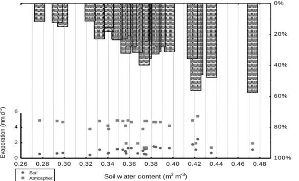
In order to better understand the depend-ency of evaporation on atmospheric demand, its relationship with the soil evaporation rate was investigated. Figure 4 shows the daily soil evaporation rate as a function of soil water
content. Soil water content shows to be signifi-cantly limiting to the evaporation rate. However, the atmosphere demand, represented here by the potential atmospheric evaporation rate, remains constant (about 1 mm from 0.24 to 0.36 m3m-3) while the relative evaporation rate increases from 10% to 20%. One might erroneously interpret that only the soil water content commands soil evaporation. Nevertheless, as previously suggested by Johns (1982) and Balwinder-Singh et al. (2014), soil evaporation is determined, for a significant part, by the atmospheric evaporative demand, even for lower water contents.
Rel at iv e ev ap o rat io n rat e (% )
Figure 4. Evaporation demand from water surface (E0) and soil surface (Es), and their ratio as a function of initial water content level
CONCLUSIONS
The results indicated that the proposed model can reasonably well estimate the daily soil evaporation rate. Errors ranged from +14% to -7% and can be attributed to the absence of non-isothermal conditions. The experimental data indicate that the atmospheric demand can significantly influence the evaporation rate even under low soil water contents.
The direct measurement of soil evaporation rate under uncontrolled condition remains difficult, costly, time consuming and
usually impractical. Nevertheless, the presented model is an easy and relatively accurate method that can be tested in irrigated areas in order to aid irrigation water management.
ACKNOWLEDGEMENTS
The São Paulo Research Foundation (FAPESP, Research Project #2013/24138-1) and the National Institute of Science and Technology on Irrigation Engineering (INCT-EI), for the financial and institutional support. 0.26 0.28 0.30 0.32 0.34 0.36 0.38 0.40 0.42 0.44 0.46 0.48
Soil w ater content (m3 m-3)
0 2 4 6 8 10 12 14 16 18 20 E va p o ra tio n ( m m d -1) 0% 20% 40% 60% 80% 100% Soil Atmospher
VARIABLES
REFERENCES
BALWINDER-SINGH.; EBERBACH, P.L; HUMPHREYS, E. Simulation of the evaporation of soil water beneath a wheat crop canopy. Agricultural Water Management, v.135, p. 19-26. 2014.
CAMPBELL, G. Soil physics with basic: transport models for soil-plant systems. Developments in Soil Science 14. 1. ed. Amsterdam: Elsevier Science, 1985. 150 p. HILLEL, D.I. 1980. Applications of soil physics. 1. ed. New York: Academic Press, 1980, 385 p.
JOHNS, G.G. Measurement and simulation of evaporation from a red earth. I. Measurement in glasshouse using a neutron moisture meter. Australian Journal of Soil Research, v.20, p. 165-178, 1982.
KROES, J.; VAN, J.C.; GROENENDIJK, D.P; HENDRIKS, R.F.A.; JACOBS, C.M.J. SWAP Version 3.2 – Theory description and user manual. The Netherlands (Wageningen): Alterra, 2008, 284 p.
METZGER, J.C.; LANDSCHREIBER, L.; GRÖNGRÖFT, A.; ESCHENBACH, A. Soil evaporation under different types of land use in southern African savanna ecosystems. Journal of Plant Nutrition and Soil Science, v.177, p. 468-475, 2014.
MONTEITH, J.L. Evaporation and surface temperature. Quarterly Journal of the Royal Meteorological Society, v.107, p. 1-27, 1981. NASH, J.C.; SUTCLIFFE, J.V. Flow river forecasting through conceptual models: I. A discussion of principles. Journal of Hydrology, v. 10, p. 282-290, 1970.
PAREDES, P.; WEI, Z.; LIU, Y.; XU, D.; XIN, T.; ZHANG, B.; PEREIRA, L.S. Performance assessment of the FAO AquaCrop model for soil water, soil evaporation, biomass and yield of soybeans in North China Plain. Agricultural Water Management, v.152, p. 57-71, 2015.
PHILIP, J.R. Evaporation, and moisture and heat fields in the soil. Journal of Meteorology, v.14, p. 354-366, 1957.
RAES, D., STEDUTO, P., HSIAO, T.C., FERERES, E. AquaCrop—the FAO crop model to simulate yield response to water II: Main algorithms and soft ware description. Agronomy Journal, v. 101, p. 438–447, 2009. RICHIE, J.T. Model for predicting evaporation from a row crop with incomplete cover. Water Resource Research, v.8, p. 1204-1214, 1972. STROOSNIJDER, L. Soil evaporation – test of a practical approach under semiarid conditions. Netherlands Journal of Agricultural Science, v.35, p. 417-426, 1987.
VANUYTRECHT, E., RAES, D., STEDUTO, P., HSIAO, T. C., FERERES, E., HENG, L. K., VILA, M. G., MORENO, P. M. AquaCrop: FAO’s crop water productivity and yield response model. Environmental Modelling & Sofware, v.62, p. 351-360, 2014.
WALLACE, J.S.; JACKSON, N.A.; ONG, C.K. Modelling soil evaporation in an agroforestry system in Kenya. Agricultural and Forest Meteorology, v.94, p. 189-202, 1999.
WEI, Z.; PAREDES, P.; LIU, Y.; CHI, W.W.; PEREIRA, L.S. Modelling transpiration, soil evaporation and yield prediction of soybean in North China Plain. Agricultural Water Management, v.147, p. 43-53, 2015.
YIOTIS, A.G.; TSIMPANOGIANNIS, I.N.; STUBOS, A.K.; YORTSOS, Y.C. Pora-net-work study of the characteristic periods in the drying of porous materials. Journal of Colloid and Interface Science, v. 297, p. 738-748, 2006.
ZAREI, C.; HOMAEE, M.; LIAGHAT, A.M.; HOORFAR, A.H. A model for soil surface evaporation based on Campbell’s retention curve. Journal of Hydrology, v. 380, p. 356-361, 2010.