242
SPECTRAL-TEMPORAL PROFILE ANALYSIS OF MAIZE, SOYBEAN AND SUGARCANE BASED ON OLI/LANDSAT-8 DATA
Bruno Montibeller 1, Ieda Del'Arco Sanches 2, Alfredo José Barreto Luiz 3, Fabio Gonçalves 4, Daniel Alves de Aguiar 5
1University of Tartu. E-mail: bruno.montibeller@ut.ee
2 National Institute for Space Research. E-mail: ieda.sanches@inpe.br
3 Embrapa Environment. E-mail: alfredo.luiz@embrapa.br
4 Canopy Remote Sensing Solutions. E-mail: fabio@canopyrss.tech
5 Agrosatélite Geotecnologia Aplicada. E-mail: daniel@agrosatelite.com.br
ABSTRACT
Remote sensing (RS) technology is a viable complementary alternative to current agriculture surveying methods. RS data spectral information is a main variable used for several purposes, such as crop type identification. However, different management practices (MP) adopted in crop cultivation may alter its spectral characteristics. The objective of this work is to analyze the spectral-temporal profile (STP) variation of soybean, maize and sugarcane cultivated under different MP. We used time series of the six spectral bands of the OLI/Landsat-8 sensor and of two vegetation indexes (VI) to investigate the intraspecific variation (same crop specie) and the interspecific variation (different crop species). We applied hierarchical cluster analyses to determine the crop’s STP variation. The bands results were more efficient than the VI. This shows that despite the widely use of VI, better results are retrieved when using the bands STP, which also allows differentiating and analyzing crops cultivated under different MP.
Keywords: Interspecific variation, intraspecific variation, agricultural dynamics, cluster analysis,
vegetation indices
ANÁLISE ESPECTRO-TEMPORAL DAS CULTURAS DE MILHO, SOJA E CANA-DE-AÇÚCAR COM DADOS DE SENSOR OLI/LANDSAT-8
RESUMO
Dados de sensoriamento remoto são uma alternativa complementar aos métodos atuais de levantamento agrícola. A informação espectral dos dados de sensoriamento remoto é a principal variável utilizada para diversos propósitos como, por exemplo, a identificação do tipo de cultura.
243 Porém, diferentes métodos de manejo (MM) adotados durante o cultivo podem alterar as características espectrais das culturas. Assim, o objetivo deste trabalho é analisar a variação do perfil espectro-temporal (PET) da soja, do milho e da cana-de-açúcar cultivadas com diferentes MM. Séries temporais de seis bandas espectrais do sensor OLI/Landsat-8 e dois índices de vegetação (IV) foram utilizados para analisar as variações intraespecíficas (mesma cultura) e interespecíficas (diferentes culturas). Para determinar as variações entre os PET das culturas, foi utilizado análises hierárquicas de clusters. Os resultados das análises baseadas nas bandas foram mais eficientes dos que as baseadas nos IV, apesar do amplo uso destes últimos.
Palavras-chave: Variação interespecífica, variação intraespecífica, dinâmica agrícola, análise de
clusters, índices de vetação
INTRODUCTION
Remote sensing (RS) data has been applied worldwide in several monitoring agricultural systems to provide, for instance, the area occupied with different crops (ATZBERGER, 2013). This sort of information helps to create better strategies regarding import and export trade and is highly important in countries such as Brazil, which has agriculture as one of the most important economic activities (JOHNSON et al., 2014). In addition, Brazil develops agricultural activities in 5,072,152 agricultural establishments totaling 350,253,329 hectares of land (IBGE, 2019) that are distributed in tropical and temperate zones of two hemispheres and four time zones, which makes monitoring these activities even more difficult.
Brazil’s soybean and maize harvested area in 2015/2016 crop year was 33.2 and 15.9 million hectares (ha), respectively. In the same period, the area cultivated with sugarcane (third major crop in area) was 7.6 million ha (CONAB, 2016). With this extensive agricultural area, approaches based on RS data are ought to complement the previously mentioned area information. It also provides the plantations geolocation, which allows a better understanding and management of the natural resources used (MELLO et al., 2010).
Studies have been using RS data acquired by different sensors and, therefore, different spatial and temporal resolutions. Due to its high temporal and moderate spatial resolution, the Moderate Resolution Imaging Spectroradiometer (MODIS) sensor has been the most applied sensor for monitoring agriculture (BROWN et al., 2007; SAKAMOTO et al., 2010). However, its
244
data cannot be applied in a major part of Brazilian agriculture area because of the crop fields size or shapes. Contrary, data acquired by sensors onboard Landsat satellites have suitable spatial resolution (30 m), but not high temporal resolution (16 days) which is a limitation in countries with high cloud incidence, such as Brazil (EBERHARDT et al., 2016).
Independently of the satellite data used, most approaches are based on images time series and their spectral information (KASTENS et al., 2017; PEÑA & BRENNING, 2015; WALDHOFF et al., 2012). The time series images provide the crop spectral-temporal profile, which allows monitoring its vegetation development from sowing to harvest time. Nonetheless, as diverse factors influence spectral information, analyses based on it are very complex. Some of these factors are crop canopy structure, crop development phase, data geometry of acquisition (illumination and view geometry), leaf area index and management practices (e.g. rain feed, irrigated, first or second harvested, no-tillage) (FERGUSON et al., 2003). The influence of these factors result in different spectral-temporal profiles for the same crop (intraspecific) or in similarities between different crops (interspecific). These differences or similarities stand as a limitation for analyses of agriculture areas based on RS data, such as crop classification (KUSSUL et al., 2016), yield estimation (JOHNSON, 2014), biomass stock (BATTUDE et al., 2016), hydric crop stress (MISHRA et al., 2015), agriculture intensification (OLIVEIRA et al., 2014), etc.
Assessments of the spectral-temporal profiles of crops cultivated under different management practices are fundamental to understand the reasons of interspecific and intraspecific spectral variability. Based on this, the objective of this study was to analyze the spectral-temporal profile variation of soybean, maize and sugarcane crops cultivated under different management practices during two crop years (2014/2015 and 2015/2016) in the mesoregion of Campinas, São Paulo, Brazil. In order to do that, we used time series images of OLI/Landsat-8 and hierarchical cluster analysis to check if the intraspecific variation of these crops are smaller than the interspecific variation.
As innovativeness, our results indicate that the use of bands spectral-temporal profiles are more efficient than the use of vegetation indices temporal profiles (which are more commonly used due to the small amount of data when compared to the bands data) for crop differentiation, independently of the management practice adopted.
245
MATERIAL AND METHODS Study area and field data
The study area comprises an overlapping region of two Landsat scenes (219/75 and 220/75) in the state of São Paulo (SP), Brazil (Figure 1). This overlapping region enables images to be obtained each 7-9 days, therefore increasing the possibility of acquiring more cloud free OLI images, and consequently more spectral information of the crops.
A segment of ~100km in the highway SP-340 was delimited on the overlapping region, passing over five municipalities (Estiva Gerbi, Aguaí, Mococa, Mogi Guaçu, and Casa Branca). The region has a flat relief with smooth hills and red and red-yellow latosols (IBGE, 2004).
Figure 1. Location of the segment in the study area and Landsat scenes (219/75 and 220/75)
overlapping region. São José dos Campos, São Paulo State, Brazil, 2019.
In the mentioned segment, 55 agricultural fields, including annual, semi-perennial, perennial crops, and silviculture, were monitored between July 2014 and December 2016. During this period, monthly campaigns were conducted to acquire information about the condition of the crops throughout their vegetation development. Examples of information acquired are crop’s species, phenological phase, and use or not of irrigation. The monitoring is one of the activities developed by the project “Development and implantation of an agriculture monitoring system for Brazil based on satellite of Earth observation data” conducted by researchers from National Institute for Space Research (INPE) and Brazilian Agricultural Research Corporation
246
(EMBRAPA). In the present work, we used the data only for soybean, maize and sugarcane fields and for the period between Oct-2014 and Jul-2016.
In the selected study area, the double-cropping production is a common practice, which means that during the two-growing seasons analyzed, four harvests were monitored for maize and soybean (annual crops). The first was from Oct-2014 to ±Mar-2015 (h1415), the second from ±Mar 2015 to ±Jul 2015 (h15), the third Oct-2015 to ±Mar-2016 (h1516), and the fourth from ±Mar 2016 to ±Jul 2016 (h16). There is no practice of double cropping of sugarcane since it is a semi-perennial crop. During the monitoring period, 29 crop fields were cultivated once or more with soybean, maize or sugarcane.
OLI/Landsat-8 images and delimitation of crop fields
In addition to field data, cloud free OLI surface reflectance images (VERMOTE et al., 2016) were downloaded from the United State Geological Survey (USGS) repository for the period from Oct-2014 to Oct-2016. For the present study, the spectral bands from the visible (Blue-B2, Green-B3 and Red-B4), near infrared (NIR-B5) and shortwave infrared regions (SWIR I-B6 and SWIR II-B7) were used. The vegetation indexes (VIs): Normalized Difference Vegetation Index – NDVI (ROUSE et al., 1972); and Enhanced Vegetation Index – EVI (HUETE et al., 1995), calculated based on the OLI bands, were also used.
A visual assessment for cloud presence in the OLI images was performed using false color composite images (R5-G6-B4). This approach provided the possibility of identifying the presence of cloud shadow as well as aerosols and cirrus clouds at crop field scale. After the assessment, we selected 54 images for our study. However, as some images had cloud cover in part of the crop fields monitored, the number of available images is not equal for every crop field. Thus, the number of images can vary even though the crop fields were cultivated during the same growing season. This allows us to use visible parts of images that are only partially contaminated by clouds, which increases the amount of observation of selected objects over time, especially when working with samples and not with the intention of building a continuous map in space.
Using the field data, cloud free OLI images and the high-resolution Google Earth imagery, we delimited the boundaries of each crop field by visual interpretation. The area homogeneity was the main criteria used to define the limits. The limits of crop fields and its OLI image time series, as well as the photos acquired during the field campaign are present in Figure 2.
247
Figure 2. Clips of OLI image time series (R5G6B4) for maize, soybean and sugarcane crop fields
and its respective photos acquired during field campaigns. São José dos Campos, São Paulo State, Brazil, 2019.
The crop fields have different sizes as well as different management systems. The smallest one has ~12ha whereas the biggest one has ~290ha. From all 28 fields, 15 used irrigation system and were cultivated with either soybean or maize in different growing seasons (common crop rotation).
After the delimitation of crop fields, time series of NDVI derived from MODIS sensor (250m) for the central coordinate of each crop field were acquired from the SatVeg platform (https://www.satveg.cnptia.embrapa.br/satveg/login.html). The Savitzky–Golay filter was applied to smooth out noise in NDVI time-series, based on window length of four.
Pixels Reflectance values extraction
Once the OLI database was established, we extracted all the pixels’ values (OLI bands) and VI’s values (NDVI and EVI) within the crop fields (Figure 3). The extraction was applied for all
248
pixels with more than 80% of overlapping by the crop fields limits. This overlapping threshold was applied to avoid border effects. Then, we calculated the median value based on all values of each band and VI. After that, we extracted only the 50 greatest and lowest than the median value (totalizing 101 values). This procedure was also applied for every OLI band and VI to avoid pixels with discrepant values. Subsequently, the mean of the 101 values was calculated for each band and VI. As a result, we acquired a mean value for each band and VI, for each crop field.
Figure 3. Example of the extraction of the reflectance values from band 5 (B5) of the OLI image
dated from 2014/10/29. São José dos Campos, São Paulo State, Brazil, 2019.
Planting date definition
The next step was to define the planting date for the crop fields, as this information could not be acquired in situ for all crop fields monitored. The planted date definition was based on the approach proposed by Fischer (1994). For that, we used the time series of NDVI/MODIS from the central coordinate of each crop field. According to Fischer (1994), the planted date is establish as the date of inflection of the NDVI time series in the beginning of the growing season. The planted date definition was essential for the next methodological procedure.
As cloud cover limited the number of images available, especially during summer growing season, there was a variation in the number of suitable images among the crop fields. To overcome this limitation, we divided the crops phenological cycle in three phases (P1, P2 and P3): P1 was defined by the planting and emergence periods (soil is the main feature of interaction with electromagnetic radiation); P2 was characterized by the vegetation development, followed by the
249 emergence of flowers and grains (more interaction of green cover with electromagnetic radiation); and P3 was defined as the period of maturation and senesce (FORMAGGIO & EPIPHANIO, 1990). The number of days for each phase and for each crop was defined based on literature review (FEHR & CAVINESS, 1977; RISSO et al., 2012; FARIAS et al., 2000; TOPPA et al., 2010) (Table 1). Due to sugarcane’s semi-perennial cycle and its harvested period, this crop has no P3.
Table 1. Number of days of each phase for soybean, maize and sugarcane. São José dos Campos,
São Paulo State, Brazil, 2019.
Crop Phase 1 (days) Phase 2 (days) Phase 3 (days)
Soybean 0-35 35-80 +80
Maize 0-35 35-90 +90
Sugarcane 0-90 +90
Based on the planted date, which corresponds to day zero, the mean value of each band and VI of the OLI images for the respective crop fields were classified as belonging to one of those phases (Table 1). For example, one OLI image was acquired 29 days after the soybean planted date, therefore the phase of the mean bands and VI values of this image is P1. After that, we determined the mean spectral value (bands and VI) for each phase based on the means (from the 101 values) of all images of the respective phase. For instance, a crop field was cultivated with soybean during h1415 and it had three images in P1, four images in P2 and one image in P3. Then, the P1 mean value (band and VI) was retrieved from the three images, the P2 mean value from the four images and P3 mean from the one image.
These mean values (of each phase) were applied in a hierarchical cluster analysis (HCA) (LANDIM, 2011). We used the Euclidian distance as the coefficient of similarity (KAUFMAN & ROUSSEEUW, 2009). The HCA results were expressed by dendrograms and only applied for the means values of the P2. This limitation (only P2) was due to the absence of images for the other phases for several crop fields. The HCA was applied in four different analysis groups. The first group was composed by the six spectral bands (B2, B3, B4, B5, B6, and B7), which were applied for intra and interspecific analysis; the second group was composed by three spectral bands (B4, B5 and B6), used only for interspecific analysis. The third was NDVI and fourth EVI, applied only for interspecific analysis.
To present the results, the crop fields were labeled as the following pattern: “crop_id_cropyear”. For instance, the label m_45_h1415 correspond to maize (m) crop and it was
250
cultivated in the first harvested year of 2014/15 (h14/15). The letters “sc”, “s” and “m” are the prefix for sugarcane, soybean and maize, respectively. The first harvests (main crop harvest) of each agricultural year monitored are represented by “h1415” and “h1516” whereas the second harvests are “h15” and “h16”. For sugarcane, we used h1 and h2, which represent first cycle and second cycle, respectively.
A threshold to divide in more similar or less similar clusters was defined based on the clustering sequence graph, which shows the Euclidian distance used for each cluster created. It means that a long value of distance used to create the following cluster can be determined as the threshold.
RESULTS AND DISCUSSION Spectral-temporal profiles
The high frequency of clouds reduced the number of useful images and, consequently, a less detailed spectral-temporal profiles of the crops analyzed (Figure 4). According to Parente et al. (2017), in 2015 around 80% of the Brazilian territory had only 12 OLI/Landsat-8 images free or partially free of clouds. The lack of images in time series, especially in key moments of crop development, decreases the efficiency of methodologies regardless its objective (e.g. yield estimation, water stress analysis, crop mapping) (FOERSTER et al., 2012; ATZBERGER, 2013; EBERHARDT et al., 2016; WHITCRAFT, et al., 2015).
Predominantly, the crops spectral-temporal profiles (Figure 4) correspond to the typical vegetation spectral profile, decreasing the values in the Red band (B4) and SWIR (B6), while increasing in the NIR band (B5) through time (accordingly to vegetative development). Near the end of the growing season, the values of the B5 and B6 start increasing whereas the B5 values decrease. For the soybean and maize, we consider that the maximum period of vegetation development is around the central part of the P2, while sugarcane has a sort of constant development in this phase. This aspect is inferred mainly in the B5 profile of each crop, once this band present more differences among crops. Due to it, a threshold (0.4) was delimited for this band (B5) to assist forthcoming analysis.
251
Figure 4. Spectral-temporal profile of B4 (red), B5 (NIR) and B6 (SWIR I) bands for maize,
soybean and sugarcane crops. Phase 1 (P1), Phase 2 (P2) and Phase 3 (P3). The dot line is the 0.4 threshold used to assist the analyses. São José dos Campos, São Paulo State, Brazil, 2019.
Interspecific analysis – six bands (B2-B7)
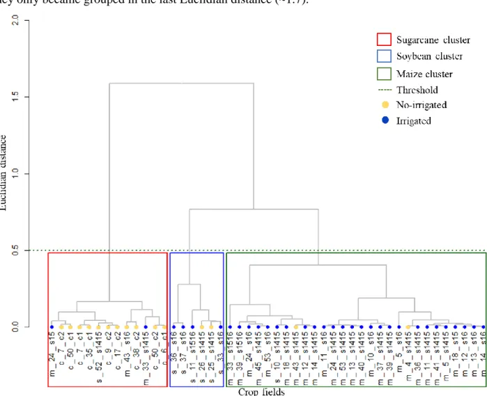
A total of 30 maize fields, 8 of soybean and 9 of sugarcane, were used in the analysis based on the mean spectral values of the six bands (B2 to B7) for the P2 (Figure 5). In general, the three clusters are mainly composed by samples of the same crop type, which means that they have similar Euclidian distance when considering the spectral characteristics of the six bands analyzed. However, some misclassification appeared. For instance, all 9 sugarcane crop fields were grouped together (red square cluster), but in the same cluster we found 3 maize and 1 soybean samples. A mainly maize-predominant cluster was formed (blue square cluster), but one soybean sample was also grouped in this cluster. Note that these misclassifications occurred independently of the crop year of the samples.
252
Another interesting aspect of the results is that even though maize and sugarcane are crops from the same taxonomic family and have similar canopy structure when compared with soybean, they only became grouped in the last Euclidian distance (~1.7).
Figure 5. Dendrogram of the interspecific analyses for maize, soybean and sugarcane fields based
on six OLI bands. São José dos Campos, São Paulo State, Brazil, 2019.
To identify possible explanations for the previous analyses, we provided an overview of the P2 mean values distribuition of the six bands among the crops in Figure 6. Some assumptions are highlighted as the explanations for the cluster formation (Figure 5). The bands B5 (NIR), B6 (SWIR I) and B7 (SWIR II) present the greatest differences, whereas the visible region bands (B2, B3 e B4) show more subtle differences. As the infrared region bands have the greatest differences, it means they had more influence in the interspecific hierarchical cluster analyses.
We also explored the spectral-temporal profile of each field individually, combining with the field data. Every crop field that was incorrectly grouped had some particular
253 characteristic/reason that explained its misclassification. All soybean and maize crop fields present in the sugarcane cluster (Figure 5) were under the threshold of 0.4 in B5 (Figure 4). This suggests that these plants had inferior vegetation development compared to the others, which was confirmed by the anotations made during field work. As can be observed in Figure 7, the s_52_h1415 sample presents a low vegetation development, which is represented by the heterogeneity of the crop field.
Figure 6. P2 mean values distribution of all bands and all crop samples. São José dos Campos, São
254
Figure 7. The plot highlighted correspond to the soybean crop field (s_52_s1415) that was
incorrectly grouped in the sugarcane cluster. São José dos Campos, São Paulo state, Brazil, 2019.
Another aspect responsible for misclassifying cluster analysis was the number of images in the P2 and their date. For example, the sample m_33_h1415 present two images in the P2, however these images are dated in the very beginning and at the very ending of the P2. It reduces the mean value of P2 for this crop field, making it similar with the sugarcane fields mean.
Interspecific cluster analysis – Three bands (B4, B5 and B6)
An interspecific cluster analysis was made using only B4 (red), B5 (NIR) and B6 (SWIR) bands. These bands are specially employed in agricultural studies based on visual interpretation of images (FORMAGGIO & SANCHES, 2017). And as demonstrated in Figure 6, these bands present the greatest differences among all spectral bands. The result of this analysis is equal to the cluster analysis involving all six bands, even the misclassifications occurred exactly with the same crop samples.
Not considering the misclassification caused by crop fields with particularities, the interspecific cluster analysis using the spectral bands (B2 to B7 or B4, B5, B6) showed efficiency and emphasize the possibility of improving classification methods, for instance. A similar assumption is shared by Peña et al. (2017) in their study. The authors used the Red, NIR and SWIR
255 bands from OLI/Landsat-8 sensor in order to classify fruitful tree species in Chile and achieved good results.
Interspecific cluster analysis – Vegetation indexes NDVI and EVI
The dendrograms in Figure 8 (A and B) present the groups established using the VIs (NDVI and EVI, respectively) mean values in the cluster analysis. The result is inferior to the analysis based on the spectral bands. Similarly, to the previous analysis using the bands, the threshold to delimit the cluster was acquired from the clustering sequence graph. The threshold was 0.5 for the NDVI results whereas for EVI the threshold was of 1.
In the analysis based on the NDVI (Figure 8A), four from eight soybean samples were incorrectly grouped, avoiding the formation of one soybean cluster. A similar tendency occurred with sugarcane crop fields samples. Among nine samples, four were incorrectly grouped. As there are more maize samples, this crop formed a cluster, however five maize samples were inadequately grouped with soybean or sugarcane.
In general, the EVI analysis (Figure 8B) has a similar pattern as the NDVI. Although there was a reduction in the misclassification between sugarcane and soybean, there was an increase for maize field samples. Three sugarcane samples and three of soybean were incorrectly grouped, while six maize samples were clustered with soybean or sugarcane.
Through the analysis of the mean P2 values distribution (Figure 9) we can infer the reasons for the misclassification in the VIs analyses (Figure 8). The distribution of NDVI mean values is more similar among maize and soybean samples when compared with sugarcane samples. This pattern is also observed in the EVI values, however with a bigger difference between sugarcane and the other crops. This difference might be influencing the formation of one sugarcane cluster in Figure 8.
256
Figure 8. A: Dendrogram of the interspecific analysis based on the NDVI mean P2 values with all
crop samples. B: Dendrogram of the interspecific analysis based on the EVI mean P2 values with all crop samples. São José dos Campos, São Paulo State, Brazil, 2019.
257
Figure 9. Distribution of the NDVI and EVI mean P2 values from all crop samples. São José dos
Campos, São Paulo State, Brazil, 2019.
The VIs results indicate that the analysis based on the spectral bands presented the best result. Although VIs are widely applied, our results show that spectral bands time series can provide additional information (subtle changes in crop spectral characteristics) that VIs times series cannot, especially for crops with similar phenological cycle (e.g. soybean and beans, maize and millet). These results are most likely related to the fact that using the bands we are exploring three different spectral regions (visible, NIR and SWIR), whereas using the NDVI and EVI we only use two spectral regions (visible and NIR). Peña et al., (2017), similarly, affirm that several methodologies employed to classify any type of crop usually use only VI, which reduce the spectral information and result in low accuracy values. In addition, Wardlow et al. (2007) also endorse that VI values are highly affected by management practices, such as irrigation and rain feed system. These management systems can imply in different VI values among areas of the same crop type.
Intraspecific cluster analysis – Six bands (B2-B7)
The aim of these analyses was to verify the spectral-temporal differences among samples of the same crop (same species), between different crop year and different management systems (e.g. no-irrigated, irrigated, first, and second harvest). All following analysis were based on the six
258
bands and the threshold of similarity were defined accordingly to the sequence cluster graph. The thresholds were 0.12 for maize, 0.21 for soybean and 0.08 for sugarcane.
In Figure 10A, we present the results involving the maize samples. It is not possible to observe any tendency of cluster involving only samples from the same crop year or same management system, despite most samples being from crop year 14/15. In addition, the number of images in the P2 did not influence the clusters, once there are clusters formed by samples with one or five images in this period. Note that one of the clusters (red cluster) is formed by the samples that were misclassified in the interspecific analysis, corroborating that these samples presented particularities when compared with the others.
In the soybean results (Figure 10B), we observed no tendency to cluster samples from the same crop year (under the threshold 0.15). Although, similarly to the maize analysis, the number of images in the P2 did not influence in the cluster’s formation.
The sugarcane analysis (Figure 10C) shows no tendency in the formation of clusters with the same samples cycle (even though they were harvested in different periods). Among the nine samples, five were grouped independently of the cycle, which supports the idea that there is no difference between the samples cultivated in different years. The number of images in the P2, as in the soybean and maize, also did not influence for cluster formation.
In general, the intraspecific analysis showed that, for the study area, the spectral-temporal differences among fields of the same crop are smaller than differences between crops, as the Euclidian distance is much smaller (maximum of ~0.3 for maize). The tendency of clustering crop fields of the same species, but with different planting date and/or management practices (single or double cropping, first or second harvest), confirm that these aspects did not present direct influence in the clustering process. However, a variety of other elements that were not covered by this study (plant density, different varieties, space of plant lines and its orientation etc.) might have influenced the clustering process.
259
Figure 10. Dendrogram of the intraspecific analysis for the maize (m) samples (A), for the soybean
(s) samples (B) and for sugarcane (sc) samples (C). All analyses were based on the six bands (B2 - B7). São José dos Campos, São Paulo State, Brazil, 2019.
We also emphasize that most of the explanations for the misclassification were only available because of the field data acquired in situ during the monitoring period. The necessity of continuous acquisition of field data is crucial to assess and analyze the errors and the limitation in
260
agricultural remote sensing. Masialeti et al. (2010) also expressed this concern in their studies. The authors used field data acquired in a specific year to extract sample training for classifiers in images of following years. Their results were not satisfactory because changes in the planting date throughout the years were responsible for the classification errors.
Based on the cluster analysis of the spectral-temporal profiles of the soybean, maize and sugarcane, we inferred that the intraspecific (same crop species) spectral variation of the bands (B2-B7) is smaller than the interspecific spectral variation (different crops species). As the clustering process was not influenced by the different management practices and planting time, we presume that these elements did not affect or result in similar spectral characteristics among different crop species. The interspecific analysis with the six and three bands, in general, provided the best results comparing to the VIs. Since the VIs used in this work are calculated using red and NIR bands only, our results highlight the importance of including the SWIR spectral region for crop differentiation.
Some spectral misclassification among crops occurred in the cluster formation using the bands, but analyzing the individual spectral-temporal profile of the field’s samples along with field information, we could identify that the main reasons for these misclassifications were the lack of cloud free images in key moments and heterogeneous crop development. While the heterogeneity of plant development might be more complicate to address, the lack of images can be minimized by using data from different sensors (multi-sensor approach), for example Landsat-like sensor data (OLI/Landsat-8 and MSI/Sentinel 2A and B).
Based on the aspects discussed in this study, it is clear the complexity and the challenge of use RS data in the range of agriculture activity. We found several constraints while analyzing only three crop species in a specific Brazilian agricultural area. Therefore, we recommend for further studies: i) analyze crops with similar spectral characteristics (e.g. soybean and beans, millet and sorghum) in order to assess if they are more susceptive to spectral changes due to management practices or planting time; ii) apply this methodology in different agricultural regions once the management practices vary between then as well as soil type, solar radiation, vegetation cycle length, etc.; and iii) use the multi-sensor approach to minimize the cloud cover problem.
261
REFERENCES
ATZBERGER, C., 2013. Advances in remote sensing of agriculture: Context description, existing operational monitoring systems and major information needs. Remote Sensing, Basel, Switzerland, v. 5, n.2, p. 949–981.
BATTUDE, M., AL BITAR, A., MORIN, D., CROS, J., HUC, M., MARAIS SICRE, C., DEMAREZ, V., 2016. Estimating maize biomass and yield over large areas using high spatial and temporal resolution Sentinel-2 like remote sensing data. Remote Sensing of
Environment, v.184, p. 668–681. Available at https://doi.org/10.1016/j.rse.2016.07.030; Access in Jan 13, 2018.
BROWN, J., JEPSON, W., KASTENS, J., WARDLOW, B., LOMAS, J., PRICE, K., 2007. Multitemporal, Moderate-Spatial-Resolution Remote Sensing of Modern Agricultural Production and Land Modification in the Brazilian Amazon. GIScience & Remote Sensing, v. 44, n. 2, p. 117–148. Available at https://doi.org/10.2747/1548-1603.44.2.117; Access in Feb 13, 2018.
CONAB – COMPANHIA NACIONAL DE ABASTECIMENTO, 2016. Acompanhamento da safra brasileira de grãos. Boletim Grãos, v. 3, n. 11, Available at: <http://www.conab.gov.br/OlalaCMS/uploads/arquivos/16_06_09_09_00_00_boletim_graos _junho__2016_-_final.pdf>. Access in February 02, 2017.
EBERHARDT, I. D. R., SCHULTZ, B., RIZZI, R., SANCHES, I. D. A., FORMAGGIO, A. R., ATZBERGER, C., LUIZ, A. J. B., 2016. Cloud cover assessment for operational crop monitoring systems in tropical areas. Remote Sensing,Basel, Switzerland, v. 8, n. 3, p. 1–14. FARIAS, J. R. B., NEPOMUCENO, A. F., NEUMAIER, N., OYA, T., 2000. Ecofisiologia: A
cultura da soja no Brasil. Embrapa Soja,Londrina, PR, v.48, p. 1-9.
FEHR, W. R., & CAVINESS, C. E., 1977. Stages of soybean development. Special Report,Ames, IA, v. 87, p. 1-13.
FERGUSON, R., RUNDQUIST, D., SHANNON, D. K., CLAY, D., KITCHEN, N., 2003. Remote Sensing for Site-Specific Crop Management, In: Precision Agriculture Basics. Madison, WI, v. 69, n. 6, p. 647–664.
FISCHER, A., 1994. A model for the seasonal variations of vegetation indices in coarse resolution data and its inversion to extract crop parameters. Remote Sensing of Environment,v. 48, n. 2, p. 220-230. Available at https://doi.org/10.1016/0034-4257(94)90143-0; Access in Feb 16, 2018.
FOERSTER, S., KADEN, K., FOERSTER, M., & ITZEROTT, S., 2012. Crop type mapping using spectral-temporal profiles and phenological information. Computers and Electronics in
Agriculture, v. 89, p. 30–40. Available at https://doi.org/10.1016/j.compag.2012.07.015; Access in Jan 22, 2018.
FORMAGGIO, A.R., SANCHES, I.D.A., 2017. Sensoriamento remoto em agricultura. Oficina de
Textos, São Paulo, 1st ed, p. 288.
FORMAGGIO, A.R., EPIPHANIO, J.C.N., 1990. Características espectrais de culturas e rendimento agrícola. São José dos Campos, INPE, n. INPE-5125-RPE/630, p. 178. Available at http://mtc-m12.sid.inpe.br/col/sid.inpe.br/iris@1912/2005/07.19.21.23.36/doc/INPE-5125-RPE-630.pdf: Access in Sep 17, 2017.
HUETE, A. R., LIU, H. Q., BATCHILY, K., LEEUWEN, W. VAN., 1995. A Comparison of Vegetation Indices over a Global Set of TM Images for EOS-MODIS, Remote Sensing of
Environment, v. 59, n. 3, p. 440-451. Available at https://doi.org/10.1016/S0034-4257(96)00112-5; Access in Feb 13, 2018.
262
IBGE, Instituto Brasileiro de Geografia e Estatística . Mapa de solos do Brasil. 2004. Available at: <ftp://geoftp.ibge.gov.br/mapas/tematicos/sistematizacao/pedologia/>. Access in April 20, 2017.
IBGE, Instituto Brasileiro de Geografia e Estatística, 2019. Censo Agropecuário 2017. Available at: https://sidra.ibge.gov.br/tabela/6635. Access in August 15, 2019.
JOHNSON, D. M., 2014. An assessment of pre- and within-season remotely sensed variables for forecasting corn and soybean yields in the United States. Remote Sensing of Environment, v.141, p. 116–128. Available at https://doi.org/10.1016/j.rse.2013.10.027; Access in Jan 29, 2018.
KAUFMAN, L; ROUSSEEUW, P.J., 2009. Finding groups in data: an introduction to cluster analysis. John Wiley & Sons, New Jersey, v. 344, 335p.
KASTENS, J. H., BROWN, J. C., COUTINHO, A. C., BISHOP, C. R., & ESQUERDO, J. C. D. M., 2017. Soy moratorium impacts on soybean and deforestation dynamics in Mato Grosso,
Brazil. PLoS ONE, v. 12, n. 4, p. 1–21. Available at
https://doi.org/10.1371/journal.pone.0176168; Access in Jan 31, 2018.
KUSSUL, N., JAVIER GALLEGO PINILLA, F., SKAKUN, S. V, LAVRENIUK, M., LEMOINE, G., MEMBER, S., SHELESTOV, A. Y., 2016. Parcel-Based Crop Classification in Ukraine Using Landsat-8 Data and Sentinel-1A Data. IEEE Journal of Selected Topics in
Applied Earth Observations and Remote Sensing, v. 9, n. 6, p. 2500–2508. Available at https://doi.org/10.1109/JSTARS.2016.256014; Access in Jan 30, 2018.
LANDIM, P.M.B., 2011. Análise estatística de dados geológicos multivariados. Oficina de
Textos. São Paulo, p. 256.
MASIALETI, I., EGBERT, S., WARDLOW, B. D., 2010. A Comparative Analysis of Phenological Curves for Major Crops in Kansas. GIScience & Remote Sensing,v. 47, n. 2, p. 241–259. Available at https://doi.org/10.2747/1548-1603.47.2.241; Access in Feb 15, 2018. MELLO, M.P., RUDORFF, B.F., ADAMI, M., RIZZI, R., AGUIAR, D.A., GUSSO, A. FONSECA, L.M., 2010, July. A simplified Bayesian Network to map soybean plantations. In
IEEE International Geoscience and Remote Sensing Symposium. p. 351-354. Available at
https://doi.org/10.1109/IGARSS.2010.5651814; Access in Jan 23, 2018.
MISHRA, A. K., INES, A. V. M., DAS, N. N., PRAKASH KHEDUN, C., SINGH, V. P., SIVAKUMAR, B., & HANSEN, J. W., 2015. Anatomy of a local-scale drought: Application of assimilated remote sensing products, crop model, and statistical methods to an agricultural drought study. Journal of Hydrology, v. 526, p.15–29. Available at https://doi.org/10.1016/j.jhydrol.2014.10.038; Access in Mar 2, 2018.
OLIVEIRA, J. C., TRABAQUINI, K., EPIPHANIO, J. C. N., FORMAGGIO, A. R., GALVÃO, L. S., & ADAMI, M., 2014. Analysis of agricultural intensification in a basin with remote sensing data. GIScience & Remote Sensing, v. 51, n. 3, p. 253–268. Available at https://doi.org/10.1080/15481603.2014.909108; Access in Jan 27, 2018.
PARENTE, L., FERREIRA, L., FARIA, A., NOGUEIRA, S., ARAÚJO, F., TEIXEIRA, L., HAGEN, S., 2017. Monitoring the Brazilian pasturelands: A new mapping approach based on the landsat 8 spectral and temporal domains. International Journal of Applied Earth
Observation and Geoinformation, v. 62, p. 135–143. Available at https://doi.org/10.1016/j.jag.2017.06.003; Access in Mar 04, 2018.
PEÑA, M. A.; BRENNING, A., 2015. Assessing fruit-tree crop classification from Landsat-8 time series for the Maipo Valley, Chile. Remote Sensing of Environment,v. 171, p. 234–244. Available at https://doi.org/10.1016/j.rse.2015.10.029; Access in Dec 04, 2017.
263 PEÑA, M. A., LIAO, R., BRENNING, A., 2017. Using spectrotemporal indices to improve the fruit-tree crop classification accuracy. ISPRS Journal of Photogrammetry and Remote
Sensing, v. 128, p. 158–169. Available at https://doi.org/10.1016/j.isprsjprs.2017.03.019; Access in Feb 21, 2018.
RISSO, J., RIZZI, R., RUDORFF, B. F. T., ADAMI, M., SHIMABUKURO, Y. E., FORMAGGIO, A. R., EPIPHANIO, R. D. V., 2012. Índices de vegetação Modis aplicados na discriminação de áreas de soja. Pesquisa Agropecuaria Brasileira, Brasília, v. 47, n. 9, p. 1317–1326.
ROUSE, J. W., HASS, R. H., SCHELL, J. A., DEERING, D. W., 1972. Monitoring Vegetation Systems in the Great Plains with ERTS. Third Earth Resources Technology Satellite-1
Symposium, Texas, v. 74, p. 309-317.
SAKAMOTO, T., WARDLOW, B. D., GITELSON, A. A., VERMA, S. B., SUYKER, A. E., ARKEBAUER, T. J., 2010. A Two-Step Filtering approach for detecting maize and soybean phenology with time-series MODIS data. Remote Sensing of Environment,v. 114, n. 10, p. 2146–2159. Available at https://doi.org/10.1016/j.rse.2010.04.019; Access in Mar 02, 2018. TOPPA, E. V. B., JADOSKI, C. J., JULIANETTI, A., HULSHOF, T., ONO, E. O., RODRIGUES,
J. D., 2010. Aspectos da fisiologia de produção da cana-de-açúcar (Saccaharum officinarum L.). Pesquisa Aplicada & Agrotecnologia, São Paulo, p. 215-221.
VERMOTE, E., JUSTICE, C., CLAVERIE, M., FRANCH, B., 2016. Preliminary analysis of the performance of the Landsat 8/OLI land surface reflectance product. Remote Sensing of
Environment, v. 185, p. 46–56. Available at https://doi.org/10.1016/j.rse.2016.04.008; Access in Feb 27, 2018.
WALDHOFF, G., CURDT, C., HOFFMEISTER, D., BARETH, G., 2012. Analysis of multitemporal and multisensor remote sensing data for crop rotation mapping.
ISPRS-Photogrammetry, Remote Sensing and Spatial Information Sciences, v. 1, p. 177–182.
Available at https://doi.org/10.5194/isprsannals-I-7-177-2012; Access in Dec 18, 2017. WARDLOW, B. D., EGBERT, S. L., KASTENS, J. H., 2007. Analysis of time-series MODIS 250
m vegetation index data for crop classification in the U.S. Central Great Plains. Remote
Sensing of Environment, v. 108, n. 3, p. 290–310. Available at https://doi.org/10.1016/j.rse.2006.11.02; Access in Jan 22, 2018.
WHITCRAFT, A. K., BECKER-RESHEF, I., KILLOUGH, B. D., JUSTICE, C. O., 2015. Meeting earth observation requirements for global agricultural monitoring: An evaluation of the revisit capabilities of current and planned moderate resolution optical earth observing missions.
Remote Sensing, Basel, v. 7, n. 2, p. 1482–1503.
Received in: August, 30, 2018 Accepted in: December, 12, 2019