Spin dynamics of the quantum XY chain and ladder in a random "eld

Physica A 332 (2004) 1 – 14

www.elsevier.com/locate/physa

Spin dynamics of the quantum

XY

chain and

ladder in a random eld

M.E.S. Nunes

_{, J.A. Plascak}

_{, J. Florencio}

30123-970 Belo Horizonte, Minas Gerais, Brazil

b_{Instituto de Fsica, Universidade Federal Fluminense, 24210-340 Niteroi, Rio de Janeiro, Brazil}

Received 25 March 2003; received in revised form 27 August 2003

Abstract

We investigate the Hamiltonian dynamics of two low-dimensional quantum spin systems in a random eld, at the innite-temperature limit: theXY chain and the two-leg XY ladder with interchain Ising interactions. We determine the longitudinal spin autocorrelation functions of the spin-1₂XY chain and ladder in the presence of disordered elds by using the method of recurrence relations. The rst six basis vectors for the chain and the rst four basis vectors for the ladder of the dynamic Hilbert spaces ofzj(t), as well as the corresponding recurrents and moments of the time-dependent autocorrelation function, are analytically computed for bimodal distributions of the elds. We did nd a remarkable result in the disordered models. Cases with a fraction of psites under eldBB and a fraction of 1−psites under the eldBA have the same longitudinal dynamics as those withpsites under eld BA and 1−p sites under the eldBB. We also nd that both theXY chain and the two-legXY ladder with Ising interchain coupling in the presence of random elds are sensitive to the percentage of disorder but not to the intensity of the elds.

c

2003 Elsevier B.V. All rights reserved.

PACS:75.40.Gb; 75.50.Lk; 75.10.Jm; 05.05.+q

Keywords:XY model; Spin dynamics; Method of recurrence relations; Continued fractions

1. Introduction

The quantum XY chain has attracted considerable attention during the last four decades not only as an interesting many-body theoretical problem but also due to

∗

Corresponding author.

E-mail addresses: eugenia@sica.ufmg.br (M.E.S. Nunes), pla@sica.ufmg.br (J.A. Plascak),

jfj@if.u.br(J. Florencio).

its applicability to real quasi-one-dimensional compounds. The Hamiltonian of the one-dimensional spin-1₂XY model can be dened by

H=1 2

N

i=1

(Jxxiix+1+Jyyi y i+1)−

1 2

N

i=1

Bizi ; (1)

where_i (=x; y; z) are Pauli matrices on site i, Jx andJy are nearest-neighbor

cou-pling constants, N is the number of sites, and Bi is the eld at site i. This model,

with Bi = 0, was introduced in 1961 and many of its properties have been

deter-mined exactly [1–4]. It has been successfully used to describe the dynamic behavior of quasi-one-dimensional compounds, such as PrCl3 [5] and CsCoCl3 [6]. Lieb et al. [1], who introduced the model, used the Jordan–Wigner transformation [7] to map the problem onto that of a system of non-interacting spinless fermions to nd the exact energies of the model. Ever since, a good deal of work has appeared in the literature concerning mainly its thermodynamic properties. Katsura [2] solved the anisotropicXY

model in the presence of a uniform magnetic eld in thez direction (i.e., Jx=Jy and Bi=B) with the help of Jordan–Wigner transformation. He obtained exact results for the

temperature and magnetic eld dependence of various thermodynamics properties such as magnetization, susceptibility, and specic heat, among others. Suzuki [8] studied the eect of a staggered magnetic eld Bi by using a theorem to calculate the partition

function exactly. A further extension on this model was done by Derzhko and Richter [9] who calculated some thermodynamic quantities for the quantum XY chain with random Lorentzian intersite interaction and transverse eld, using the Jordan–Wigner transformation.

Regarding the dynamics of this model, Niemeijer [10] obtained the exact time-dependent correlation function C(t) =z

j(0)zj(t) at T → ∞ and Bi = 0 for the

isotropic model (Jx=Jy). The result is simply C(t) = [J0(2t)]2, whereJ0 is the zeroth order Bessel function. McCoy [11] studied the spatial spin pair correlation function along thex, y, and z directions for dierent anisotropies in the limit of large number of sites. AtT = 0, those correlation functions decay to zero exponentially as the num-ber of spinsN → ∞. On the other hand, at T = 0 the transverse correlation function decays exponentially to a non-zero value if its direction is along that of the stronger coupling, while the other transverse correlation function approaches zero exponentially asN → ∞. In the isotropic case, all three correlation functions approach zero following power laws, asN → ∞.

Barouch et al. [12–14] studied the time-dependent properties of the z-direction magnetization. They considered theXY model in thermal equilibrium at temperatureT

in the presence of a uniform external magnetic eld B1. At t= 0, the eld is changed to some other value B2, and Mz(t) is then determined. The most interesting aspect is

that ifB2= 0, then Mz(t)= 0 as t→ ∞. They also examined the asymptotic behavior

Lee [18] investigated the dynamics of the one-dimensional s=1

2 isotropic XY model and the transverse Ising model in the high-temperature limit by using the method of recurrence relations. They found that the dynamic Hilbert spaces of the two models have the same structure, which leads to a similar dynamic behavior apart from a time scale.

Quantum models dened on a ladder structure have also been of considerable in-terest since they can be viewed as an interpolation between one- and two-dimensional systems. Physical realizations such as (VO)2P2O7 [19] and Cu2(C5H12N2)2Cl4[20] cor-respond in fact to quantum Heisenberg ladders. The full two-leg ladder Heisenberg– Ising Hamiltonian can be written as

H=1 2

N

i=1

(Jxxi;1xi+1;1+Jyyi;1 y

i+1;1+Jzi;z1iz+1;1)

+1 2

N

i=1

(Jxxi;2ix+1;2+Jyi;y2 y

i+1;2+Jzi;z2zi+1;2)

+1 2

N

i=1

Iii;z1zi;2− 1 2

N

i=1

Bi;1zi;1− 1 2

N

i=1

Bi;2zi;2; (2)

where subscripts 1 and 2 refer to chains 1 and 2, J (=x; y; z) are exchange

cou-plings, Ii is the interchain Ising coupling, and Bi;1 and Bi;2 are external elds. Most

of the theoretical work with spin ladders deals with ladders with Heisenberg or XXZ

interactions along the legs. Only a few of them concern the case whereJz= 0, that is,

the XY-Ising ladder. Huber and Caille [21] studied the XY-Ising ladder consisting of two chains, with Jx=Jy, connected by a uniform Ising interaction I. They used the

Jordan–Wigner transformation to obtain the specic heat. Hikihara and Furusaki [22] numerically computed the spatial correlation functions along the xand z directions by using the density matrix and renormalization group approaches. Orignac and Giamarchi [23] treated anisotropic spin-1₂XY ladders in the presence of several types of weak ran-dom perturbations. They found that the eect of the disorder depends on whether or not theXY symmetry is preserved. More recently, Melin et al. [24] considered ladders with a strong disorder in the antiferromagnetic interactions.

In this paper, we study the eects of an applied random eld on the dynamic be-havior at the innite-temperature limit of the longitudinal autocorrelation function of the following spin-1₂ systems: (i) the XY model in one dimension, and (ii) the two-leg

XY-Ising ladder. In both cases, the elds Bi are drawn independently according to

This paper is arranged as follows. In Section2 we review the method of recurrence relations. In Section 3 that method is applied to study the dynamical behavior of the

XY chain in a disordered eld. Our study of the dynamics of the XY-Ising ladder is presented in Section4. Finally, in Section 5 we summarize our results.

2. Method of recurrence relations

Consider a system described by a HamiltonianH. The time evolution of an operator

A is governed by dA(t)

dt = iLA(t); (3)

whereL is the Liouville operator, dened byLA= [H; A]≡HA−AH. The solution to Eq. (3) can be cast as the following orthogonal expansion

A(t) =

d−1

n=0

an(t)fn ; (4)

where thefn’s are basis vectors spanning a d-dimensional Hilbert space S. In order to

include an average over disorder, we now modify the original denition of the scalar product, that is, we dene the scalar product in S as the Kubo product [41] averaged over the random variables

(X; Y) = 1

0

dX()Y† _{− XY}†_{; (5)}

where· · · denotes an ensemble average and an average over all realizations of dis-order. Here, X and Y are vectors dened in S, = 1=kBT is the inverse temperature,

and X() = exp(H)Xexp(−H). In the high-temperature limit, T → ∞, the scalar product reduces to

(X; Y) =TrXY †

Tr1 ; (6)

where Tr1 gives the number of states of the system.

By choosingf0=A(0), it follows that the remaining basis vectors can be generated

by using the following recurrence relation:

fn+1= iLfn+nfn−1 ; (RRI)

where 06n6d−1. The quantity

n=

(fn; fn)

(fn−1; fn−1)

; n¿1 (7)

gives the relative norms of consecutive basis vectors, and is usually referred to as recurrent. By denition, f−1≡0 and 0≡1.

The coecients an(t)s satisfy a second recurrence relation

n+1an+1(t) =−

dan(t)

where 06n6d−1, and a−1(t)≡0. Notice that with the initial choice f0=A(0), it

follows from Eq. (4) that a0(0) = 1, and an(0) = 0 for n¿1. Hence, a0(t) represents the relaxation function of linear response theory. In the limit T → ∞, a0(t) is simply the time-dependent autocorrelation functionC(t). The complete time evolution of A(t) can thus be determined by using (RRI) and (RRII).

By applying the Laplace transform to (RRII), one obtains

11(z) = 1−z0(z); n= 0; (8)

n+1n+1(z) =−zn(z) +n−1(z); n¿1; (9)

where

n(z) =

∞

0

e−ztan(t) dt; Rez ¿0: (10)

By using Eqs. (8) and (9), one obtains the continued fraction for 0(z):

0(z) =

1

z+ (1=z+ (2=z+· · ·))

: (11)

Note that the n are the sole ingredients that enter the determination of the dynamic

correlation functions. In addition, the knowledge of the n enables one to obtain the

moments of the correlation function. In practice, only a few n can be determined

analytically.

By working on the high-temperature limit, T =∞, we managed to obtain the rst six n pertaining to zj(t) and Hamiltonian (1), and the rst four n for

Hamilto-nian (2). From the n, we determine the corresponding moments 2n of the average

time-dependent correlation function

C(t) =z

j(0)zj(t)= ∞

k=0

2kt2k ; (12)

where2k are dened by the following formula involving 2k nested commutators,

2k=

1 2k!(−1)

k_{[H;[H; : : :[H;} z

j]· · ·]]zj: (13)

It is also possible to compute the spectral function(!) which is dened as the Fourier transform of the time-dependent autocorrelation function

(!) =

∞

−∞

ei!tC0(t) dt : (14)

This spectral function has the advantage of being accessible in experiments.

3. Dynamics of theXY chain in a random eld

In this section, we focus on the spin autocorrelation function of theXY model in one dimension in the innite-temperature limit. Hamiltonian (1) is given by the following, in the isotropic case (Jx=Jy=J),

H=J 2

N

i=1

(_ixx_i+1+_iyy_i+1)−1 2

N

i=1

where the elds Bi are randomly drawn according to the bimodal distribution

({Bi}) = N

i

[p(Bi−BA) + (1−p)(Bi−BB)] (16)

with 06p61, where p represents the probability of drawing BA. Thus p= 0 and

p= 1 correspond to the cases Bi=BB andBi=BA, respectively. We shall be interested

in the cases where BA= 0 and BB= 1:5J. The distribution is normalized to unity

and the average of a given function f({Bi}) is obtained simply by using the integral

f({Bi}) =

∞

−∞

({Bi})f({Bi}) N

i

dBi : (17)

Since we are interested in the longitudinal correlation function in the limit of innite temperature, Eq. (12), we express the time evolution of the tagged spinz

j as follows:

z_j(t) =

d−1

n=0

an(t)fn; (18)

where f0=z

j(0) =zj. Clearly, (f0; f0) = (zj; zj) = 1. The other basis vectors are

determined using the recurrence relation (RRI). Thus for f1, we obtain

f1=Jyjxj+1+Jxj−1 y j −Jjx

y j+1−J

y j−1

x

j : (19)

Its squared norm is computed by using theT=∞limit of Kubo product, Eq. (6). The result is

(f1; f1) = 4J2 ; (20)

which already includes the average over the random elds. After a somewhat lengthy but straightforward calculation, we exactly determined the vectors f2, f3; : : : ; f6. The

results are rather involved and shall not be reported here. The rst recurrent is readily determined,

1=

(f1; f1)

(f0; f0)= 4J

2 _{: (21)}

Notice that it does not depend on the external magnetic elds BA or BB. The next

recurrent is

2= 5J2+ 2[pB2A+ (1−p)B2B]−2[pBA+ (1−p)BB]2 ; (22)

which now depends on bothBAandBB. By following this procedure, we also calculated

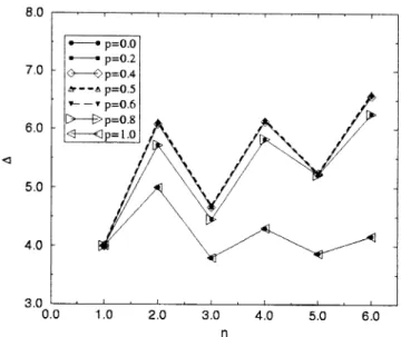
3; : : : ; 6. The results, however, are again too lengthy to be reproduced here. Rather, we present the results for the recurrents in Fig. 1. They are shown for n66 and dierent concentrationspof BA= 0, and are valid in the high-temperature limitT=∞.

Fig. 1. Recurrants, in the innite-temperature limit, for several values ofp. In the gure,BA= 0,BB= 1:5J, andJ= 1. The lines are just guides to the eye.

In order to determine the time-dependent autocorrelation function at T =∞, de-ned by Eq. (12), one must have the moments 2k or, equivalently, the recurrents n. Usually, when just a few of the recurrents are available, one can only nd the

short-time expansion ofC(t). In order to extend the region of validity to longer times, we propose an ansatz for n, n ¿6. Such approach relies strongly on the behavior of

the known recurrents. For the isotropic XY chain in the absence of an applied eld, it can be shown from the exact result of Ref. [10] that the recurrents tend to a nite value ∞= 4J2 as n → ∞. In the present case, the results of Fig. 1 suggest that

the recurrents also approach a nite value as n gets larger, even in the disordered cases 0¡ p ¡1 (recall thatp= 0 and 1 are disorderless cases). We shall assume that both the odd- and even-ordered recurrents approach a common terminal value ∞ by

following independent power-laws, just like in the case of the isotropic XY chain. Based on the above considerations, we can construct an approximant to the higher-order recurrents in the innite-temperature limit: (i) rst, we estimate the value of∞

by plotting n versus 1=n and assuming that ∞ is given by its extrapolated value at

the origin of the horizontal axis (as n → ∞); (ii) next, we use the following ansatz for the high-ordered recurrents,

n= A

n +∞; n= 1;3;5; : : : ; (23)

A= (3−∞)3 ; (24)

=−ln

∞−5

∞−3

ln

5 3

Table 1

Parameters of the ansatz for the recurrents in the innite-temperature limit, Eqs. (23)–(28). We usedBA= 0, BB= 1:5J, andJ= 1

p ∞ A B

0.0 and 1.0 4.15 −0:58 0.45 −0:58 0.45

0.2 and 0.8 6.05 −0:49 0.56 −6:53 1.28

0.6 and 0.4 6.34 −0:33 0.28 −4:16 0.83

0.5 6.37 −0:28 0.17 −3:99 0.78

and

n=

B

n +∞; n= 2;4;6; : : : ; (26)

B= (4−∞)4 ; (27)

=−ln

∞−4

∞−6

ln

3 2

: (28)

The parameters ∞, A, , B, and , which appear in the ansatz above, are listed in Table1for several values ofp, forBA= 0,BB= 1:5J,J= 1, in the innite-temperature

limit.

It is worthwhile to compare the outcomes of our extrapolation scheme above with a known exact result, so that one can attest the reliability of the method. Consider the XY chain with isotropic interactions Ji=J, in the absence of external elds, in

the innite-temperature limit, that is, the system for which Niemeijer’s solution applies. The recurrentsn, derived from that solution,J0(2Jt)2, oscillate about a terminal value

∞= 4J2 as n grows, with decreasing amplitude. Both the odd and even recurrents

ultimately reach∞ (atn=∞) by following independent power laws. We need at least

the rst 60 exact recurrents to reconstruct J0(2Jt)2 in the time region 06t610 (in units ofJ−1_{), such that no visible dierence can be seen in the scale of the gures used} in this work. Extensions for largert can be obtained by using more recurrents. Now, the present approach yields ∞= 4:15J2 (see Table 1), which is marginally higher

than the exact value. Thus, the recurrents from the ansatz tend to the terminal value with a slower power-laws ofn, as compared to the exact recurrents. The implications of these on the time-dependent correlation function are shown in Fig. 2 which shows the results from our ansatz for the XY case in comparison to the exact solution. One can clearly see that, despite the fact that our approximation is based on six exact recurrents only, we obtain good quantitative results for times up to t= 4:5. The behavior of the approximation for t¿4:5 has the same general behavior as the exact one, except that

Fig. 2. Comparison between exact and approximate autocorrelation function for the pureXY model with or without a uniform eld (i.e.,p= 0 orp= 1) atT=∞. Both curves were drawn by considering the rst 60 recurrents only.

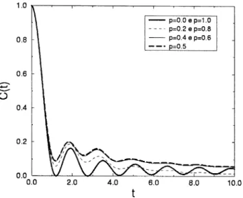
Fig. 3. Time-dependent autocorrelation function of theXY chain in the innite-temperature limit for several values ofp, where we useBA=0, BB= 1:5J (J= 1).

each other, as shown in Fig.2, we conclude that the presence or not of a uniform eld does not alter the autocorrelation function.

Fig. 4. Spectral density function of theXY chain in the limit of high temperature,T=∞, for several values ofp. Here,BA= 0,BB= 1:5J, andJ= 1.

appreciably, thereby producing slower decay at larget. Such eect is most pronounced at maximum disorder,p= 0:5. The disorder-induced raise ofC(t) is already noticeable at short times, where the curves are essentially exact. The system presents an interesting behavior when a random external eld is applied: it is susceptible to the percentage of disorder, but not to the intensity of the eld. For example, the casesp=0:2 and 0.8 have the same behavior, although the percentage of sites under the eect of external eld is dierent. Similar results are obtained for other values ofBA and BB. The explanation

is given in next section, since it also applies to the case of a ladder.

4. Dynamics of theXY-Ising ladder in a random eld

We now consider the dynamics of the two-leg spin ladder on a random eld in the high-temperature limit,T=∞. We set Jx=Jy=J andJz= 0 in Hamiltonian (2). The

external elds act on sites of both legs of the ladder. We consider two independent random eld variables,Bi;1 andBi;2, distributed according to

({Bi;1}) = N

i

[q(Bi;1−BA) + (1−q)(Bi;1−BB)]; (29)

({Bi;2}) =

N

i

[r(Bi;2−BC) + (1−r)(Bi;2−BD)]; (30)

where 06q, r61. The quantities BA and BB are random elds on chain 1, while

Fig. 5. Autocorrelation function of theXY model on a ladder without external eld (BA=BB=BC=BD= 0) and isotropic exchange interactions,J= 1, for a few values of the Ising interchain couplingI (in units of J), in the innite-temperature limit.

as in Section 3 to investigate the longitudinal dynamic spin autocorrelation functions on the ladder, C(t) =z

j(0)zj(t). We analytically determine the rst four recurrents

only, since the higher connectivity of the ladder makes the calculations much longer than those of the chain. We then use a similar procedure as in the previous section to extrapolate to longer timest. Next, we devise an ansatz similar to Eqs. (23)–(28), to estimate the next 56 recurrents. We do not present the details here since the ansatz can be easily reproduced by following the steps outlined in the last section. The only dierence is that now we have only four exact recurrents, thus making the ensuing extrapolation less reliable. Nevertheless, as we shall see, the method works remarkably well and we obtain sensible results for the autocorrelation functions.

We now outline the results for the time-dependent autocorrelation functions in the

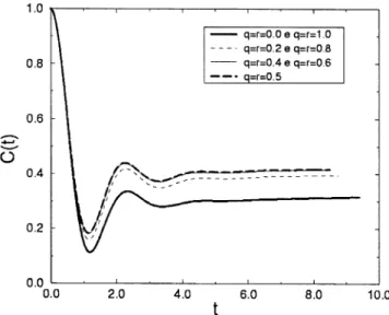
Fig. 6. Autocorrelation function for theXY model on a ladder with disordered elds (BA=BC= 0 and BB=BD= 1:5J) forJi;1=Ji;2=J=I= 1, atT=∞.

and∞. One should bear in mind that the long-time behavior shown in Fig. 5 is very likely to be a bit overestimated due to same reasons described in the last section. For example, the steady rise inC(t) at larget is surely an artifact of the ansatz used. Still our conclusions above should hold true, since the raises of C(t) due to uncertainties in the ansatz, are much smaller than the eects of the interchain coupling, especially from moderateI ∼J to higher couplings I ¿ J.

Fig. 6 shows C(t), in the innite-temperature limit, for dierent concentrations of equal elds on each chain (as well as equal concentrations on each chain). The cou-plings J=I, while the elds Bi are disordered and obey bimodal distributions, with

probabilitiesq andrfor zero eld, otherwiseBi= 1:5J. We can see that, as in the case

of the single chain model, the presence or not of an external eld produces the same dynamic behavior for the disorderless cases (p= 0 and 1). The same holds true for the symmetric pairs of distributions (q, 1−q) and (r, 1−r). Such result is due to the up–down symmetry of the model Hamiltonian along the z-direction. This symmetry is best seen with the canonical transformation of x_i →y_i, y_i →x_i, _iz → −_iz, which changes the sign of the interaction energy with the longitudinal eld and, of course, leaves the energy spectrum unchanged. Hence, a eld applied to either the positive or negative direction of the z-axis will yield the same results for both the static and dynamic quantities. Suppose we exchange the probabilities q and 1−q, as well as r

show in Fig.6. These considerations are quite general and apply to any space dimen-sions. The Ising couplingI=J already leads to non-zero long-time behavior forC(t), however disorder also liftsC(t), with highest values at maximum disorder, q=r= 0:5. Similar results are obtained for dierent values of the Ising interchain couplingI.

5. Conclusions

We investigated the time evolution of the spin-1₂ XY isotropic model dened on a single chain and on a two-leg ladder (with Ising-type interchain couplings), at innite temperature, by using the method of recurrence relations. We exactly determined the rst six moments (for the model on a chain) and the rst four moments (for the model on a ladder) of the time-dependent longitudinal correlations in the high-temperature limit. We extended the exact results, which are valid for short times only, by using an approximate method in which the recurrents are assumed to oscillate towards a terminal value ∞. Within this scheme, we were able to reproduce fairly well-known

exact results, such as the XY chain without applied eld. The most interesting aspect of the present results is the dependence of the chain and the ladder under a disordered eld. Both are sensible to the percentage of disorder, but not to the intensity of the elds. Despite its simplicity in using just a few exact recurrents, the present approach is able to give a good picture of the dynamics of the XY chain and ladder in the presence of random elds.

Acknowledgements

This work was partially supported by CNPq, FAPEMIG, and PRONEX (Brazilian agencies).

References

[1] E. Lieb, T. Schultz, D.C. Mattis, Ann. Phys. (N.Y.) 16 (1961) 407. [2] S. Katsura, Phys. Rev. 127 (1962) 1508.

[3] S. Katsura, T. Horiguchi, M. Suzuki, Physica 46 (1970) 67. [4] J.H.H. Perk, H.W. Capel, Physica 89 A (1977) 265.

[5] E. Goovaerts, H. De Raedt, D. Schoemaker, Phys. Rev. Lett. 52 (1984) 1649. [6] M. Mohan, G. Muller, Phys. Rev. B 27 (1983) 1776.

[7] P. Jordan, E. Wigner, Z. Phys. 47 (1928) 631. [8] M. Suzuki, J. Phys. Soc. Jpn. 21 (1966) 2140. [9] O. Derzhko, J. Richter, Phys. Rev. B 55 (1977) 14298. [10] Th. Niemeijer, Physica 36 (1967) 377;

Th. Niemeijer, Physica 39 (1968) 313. [11] B.M. McCoy, Phys. Rev. 173 (1968) 531.

[12] E. Barouch, B.M. McCoy, M. Dresden, Phys. Rev. A 2 (1970) 1075. [13] E. Barouch, B.M. McCoy, Phys. Rev. A 3 (1971) 786;

E. Barouch, B.M. McCoy, Phys. Rev. A 3 (1971) 2137.

[15] A. Sur, D. Jasnow, I.L. Lowe, Phys. Rev. B 12 (1975) 3845. [16] U. Brandt, K. Jacoby, Z. Phys. B 25 (1976) 181.

[17] H.W. Capel, J.H.H. Perk, Physica 87 A (1977) 211. [18] J. Florencio, M.H. Lee, Phys. Rev. B 35 (1987) 1835.

[19] D.C. Johnston, J.W. Johnston, D.P. Goshorn, A.J. Jacobson, Phys. Rev. B 35 (1987) 219. [20] M. Hagiwara, H.A. Katori, U. Schollwock, H.J. Mikeska, Phys. Rev. B 62 (2000) 1051. [21] L. Hubert, A. Caille, Phys. Rev. B 43 (1991) 13,187.

[22] T. Hikihara, A. Furusaki, Phys. Rev. B 63 (2001) 1,34,438. [23] E. Orignac, T. Giamarchi, Phys. Rev. B 57 (1998) 5812.

[24] R. Melin, Y.C. Lin, P. Lajko, H. Rieger, F. Igloi, Phys. Rev. B 65 (2002) 1,04,415. [25] M.H. Lee, Phys. Rev. Lett. 49 (1982) 1072;

M.H. Lee, Phys. Rev. B 26 (1982) 2547; M.H. Lee, J. Math. Phys. 24 (1983) 2512.

[26] M.H. Lee, J. Hong, J. Florencio, Physica Scripta T19 (1987) 498. [27] M.H. Lee, Phys. Rev. E 61 (2000) 3571.

[28] M.H. Lee, Phys. Rev. E 62 (2000) 1769.

[29] J. Florencio, S. Sen, M.H. Lee, Braz. J. Phys. 30 (2000) 725. [30] M.H. Lee, Phys. Rev. Lett. 51 (1983) 1227.

[31] J. Hong, M.H. Lee, Phys. Rev. Lett. 55 (1985) 2375. [32] J. Hong, M.H. Lee, Phys. Rev. Lett. 70 (1993) 1972.

[33] J. Florencio, O.F. de Alcantara Bonm, Phys. Rev. Lett. 72 (1994) 3286. [34] J. Florencio, S. Sen, Z.X. Cai, J. Phys.: Condens. Matter 7 (1995) 1363. [35] J. Florencio, F.C. Sa Barreto, Phys. Rev. B 60 (1999) 9555.

[36] J. Florencio, M.H. Lee, Phys. Rev. A 31 (1985) 3231. [37] I. Sawada, Phys. Rev. Lett. 83 (1999) 1668.

[38] J. Kim, I. Sawada, Phys. Rev. E 61 (2000) R2172.

[39] U. Balucani, M.H. Lee, V. Tognetti, Phys. Rep. 373 (2003) 409. [40] M.H. Lee, Phys. Rev. Lett. 87 (2001) 25061.