Simulating CO<sub>2</sub> profiles using NIES TM and comparison with HIAPER Pole-to-Pole Observations

(1)

ACPD

15, 6745–6770, 2015

Simulating CO2

profiles using NIES TM

C. Song et al.

Title Page

Abstract Introduction

Conclusions References

Tables Figures

◭ ◮

Back Close

Full Screen / Esc

Printer-friendly Version

Interactive Discussion

Discussion

P

a

per

|

Discussion

P

a

per

|

Discussion

P

a

per

|

Discussion

P

a

per

|

Atmos. Chem. Phys. Discuss., 15, 6745–6770, 2015 www.atmos-chem-phys-discuss.net/15/6745/2015/ doi:10.5194/acpd-15-6745-2015

This discussion paper is/has been under review for the journal Atmospheric Chemistry and Physics (ACP). Please refer to the corresponding final paper in ACP if available.

Simulating CO

2

profiles using NIES TM

and comparison with HIAPER

Pole-to-Pole Observations

C. Song1, S. Maksyutov2, D. Belikov2, H. Takagi2, and J. Shu1

1

Key Laboratory of Geographic Information Science, Institute of Climate Change, East China Normal University, Shanghai 200241, China

2

National Institute for Environmental Studies, Tsukuba 305-8506, Japan

Received: 26 January 2015 – Accepted: 28 January 2015 – Published: 6 March 2015 Correspondence to: C. Song ([email protected])

(2)

ACPD

15, 6745–6770, 2015

Simulating CO2

C. Song et al.

Title Page

Tables Figures

◭ ◮

Back Close

Full Screen / Esc

Discussion

P

a

per

|

Discussion

P

a

per

|

Discussion

P

a

per

|

Discussion

P

a

per

|

Abstract

We present a study on validation of the National Institute for Environmental Studies Transport Model (NIES TM) by comparing to observed vertical profiles of atmospheric CO₂. The model uses a hybrid sigma-isentropic (σ–θ) vertical coordinate that employs both terrain-following and isentropic parts switched smoothly in the stratosphere. The

5

model transport is driven by reanalyzed meteorological fields and designed to simu-late seasonal and diurnal cycles, synoptic variations, and spatial distributions of at-mospheric chemical constituents in the troposphere. The model simulations were run for biosphere, fossil fuel, air–ocean exchange, biomass burning and inverse correction fluxes of carbon dioxide (CO₂) by GOSAT Level 4 product. We compared the NIES

10

TM simulated fluxes with data from the HIAPER Pole-to-Pole Observations (HIPPO) Merged 10 s Meteorology, Atmospheric Chemistry, and Aerosol Data, including HIPPO-1, HIPPO-2 and HIPPO-3 from 128.0◦_{E to}

−84.0◦W, and 87.0◦N to−67.2◦S.

The simulation results were compared with CO2observations made in January and

November 2009, and March and April 2010. The analysis attests that the model is

15

good enough to simulate vertical profiles with errors generally within 1–2 ppmv, except for the lower stratosphere in the Northern Hemisphere high latitudes.

1 Introduction

Atmospheric carbon dioxide (CO₂) is the primary radiative forcing greenhouse gas produced by human activities. It causes the most global warming (IPCC, 2013) and

20

its atmospheric concentration has been increasing at a progressively faster rate each decade because of rising global emissions (Raupach et al., 2007). The monitoring of atmospheric CO2 from space is intended to identify the sources and sinks of the

greenhouse gases generated by human and natural activities. A number of satellites are actively monitoring greenhouse gases (e.g., GOSAT, SCIAMACHY, AIRS, IASI) to

25

(3)

ACPD

15, 6745–6770, 2015

Simulating CO2

C. Song et al.

Title Page

Tables Figures

◭ ◮

Back Close

Full Screen / Esc

Discussion

P

a

per

|

Discussion

P

a

per

|

Discussion

P

a

per

|

Discussion

P

a

per

|

satellite observation data to provide more accurate estimates of CO₂ concentrations using several different methods.

The sparseness and spatial inhomogeneity of the existing surface network have limited our ability to understand the quantity and spatiotemporal distribution of CO₂ sources and sinks (Scholes et al., 2009). Recent studies of global sources and sinks

5

of greenhouse gases, and their concentrations and distributions, have been mainly based on in situ surface measurements (GLOBALVIEW-CO₂, 2010). The diurnal and seasonal “rectifier effect”, the covariance between surface fluxes and the strength of vertical mixing, and the proximity of local sources and sinks to surface measurement sites all have an influence on the measured and simulated concentrations, and

compli-10

cate the interpretation of results (Denning et al., 1996; Gurney et al., 2004; Baker et al., 2006). Comparatively speaking, the vertical integration of mixing ratio divided by sur-face pressure, denoted as the column-averaged dry-air mole fraction (DMF; denoted XG for gas G) is much less sensitive to the vertical redistribution of the tracer within the atmospheric column (e.g., due to variations in planetary boundary layer (PBL) height)

15

and is more easily related to the underpinning surface fluxes than are near-surface concentrations (Yang et al., 2007). Thus, column-averaged measurements and simu-lations are expected to be very useful for improving our understanding of the carbon cycle (Yang et al., 2007; Keppel-Aleks et al., 2011; Wunch et al., 2011). In addition, at-mospheric transport has to be accounted for when analyzing the relationships between

20

observations of atmospheric constituents and their sources/sinks near the earth’s sur-face or through the chemical transformation in the atmosphere. As a result, reliable estimates of climate change depend upon our ability to predict atmospheric CO₂ con-centrations, which requires further investigation of the CO2sources, sinks, and

atmo-spheric transport.

25

Global atmospheric tracer transport models are usually applied to studies of the global cycles of the long-lived atmospheric trace gases, such as CO2 and methane

(CH4), because the long-lived atmospheric tracers exhibit observable global patterns

(4)

ACPD

15, 6745–6770, 2015

Simulating CO2

C. Song et al.

Title Page

Tables Figures

◭ ◮

Back Close

Full Screen / Esc

Discussion

P

a

per

|

Discussion

P

a

per

|

Discussion

P

a

per

|

Discussion

P

a

per

|

chemistry transport models (hereafter referred to as CTMs), driven by actual meteo-rology from numerical weather predictions, and global circulation models (GCMs) play a crucial role in assessing and predicting change in the composition of the atmosphere due to anthropogenic activities and natural processes (Rasch et al., 1995; Jocob et al., 1997; Denning et al., 1999; Bregman et al., 2006; Law et al., 2008; Maksyutov et al.,

5

2008; Patra et al., 2008).

The transport modeling is done on different scales ranging from local plume spread, regional mesoscale transport to global scale analysis, depending on the scale of the phenomena that are studied. Forward modeling is used to estimate tracer concentra-tions in regions that lack observation data and to identify the features of tracer transport

10

and dispersion (Law et al., 2008; Patra et al., 2008). Inverse methods are generally ap-plied when interpreting the data, with atmospheric transport models providing the link between surface gas fluxes and their subsequent influence on atmospheric concen-trations (Rayner and O’Brien, 2001; Patra et al., 2003a, b; Gurney et al., 2004; Baker et al., 2006). Global modeling analysis has helped to identify the relative contribution

15

of the land and oceans in the Northern and Southern Hemispheres to the interhemi-spheric concentration di_fferences in CO₂, CH₄, carbon monoxide (CO) and other tracer species (Bolin and Keeling, 1963; Hein et al., 1997). For stable and slowly reacting chemical species, a number of studies have derived information on the spatial and temporal distribution of the surface sources and sinks by applying a transport model

20

and atmospheric observations (Tans et al., 1990; Rayner et al., 1999).

There are several factors that strongly influence model performance: the numerical transport algorithm used, meteorological data, grid type and resolution. In tracer trans-port calculations, semi-Lagrangian transtrans-port algorithms are often used in combination with finite-volume models. Losses in the total tracer mass are possible in these

algo-25

(5)

ACPD

15, 6745–6770, 2015

Simulating CO2

C. Song et al.

Title Page

Tables Figures

◭ ◮

Back Close

Full Screen / Esc

Discussion

P

a

per

|

Discussion

P

a

per

|

Discussion

P

a

per

|

Discussion

P

a

per

|

remains a possibility of predicting distorted tracer concentrations. By contrast, when using a flux-form transport algorithm, the total tracer mass is conserved and thus the issue of mass losses can be eliminated, provided the flow is conservative. The use of numerical schemes with limiters leads to distorted tracer concentrations and affects the linearity. Thus, to accurately calculate the tracer concentration in a forward

simula-5

tion and to use the model in inverse modeling, we employed a flux-form version of the global off-line, three-dimensional chemical NIES TM.

The synoptic and seasonal variability in XCO2is driven mainly by changes in surface

pressure, the tropospheric volume-mixing ratio (VRM) and the stratospheric concentra-tion, which is affected in turn by changes in tropopause height. The effects of variations

10

in tropopause height are more pronounced with increasing contrast between strato-spheric concentrations. Many CTMs demonstrate some common failings of model transport in the stratosphere (Hall et al., 1999). The difficulty of accurately represent-ing dynamical processes in the upper troposphere (UT) and lower stratosphere (LS) has been highlighted in recent studies (Mahowald et al., 2002; Wauch and Hall, 2002;

15

Monge-Sanz et al., 2007). While there are many contributing factors, the principal fac-tors a_ffecting model performance in vertical transport are meteorological data and the vertical grid layout (Monge-Sanz et al., 2007).

The use of different meteorological fields in driving chemical transport models can lead to diverging distribution of chemical species in the UTLS region (Douglass et al.,

20

1999). The quality of wind data provided by numerical weather predictions is another crucial factor for tracer transport (Jöckel et al., 2001; Stohl et al., 2004; Bregman et al., 2006). Wind fields produced by the Data Assimilation System (DAS) are commonly used for driving CTMs. Spurious variability, or “noise”, introduced via the assimilation procedure affects the quality of meteorological data through a lack of suitable

obser-25

(6)

strato-ACPD

15, 6745–6770, 2015

Simulating CO2

C. Song et al.

Title Page

Tables Figures

◭ ◮

Back Close

Full Screen / Esc

Discussion

P

a

per

|

Discussion

P

a

per

|

Discussion

P

a

per

|

Discussion

P

a

per

|

sphere. A lack of observations makes this region the most challenging in terms of data assimilation. Bregman et al. (2006) found that the modeled vertically integrated mass change obtained for the tropical atmosphere is not in geostrophic balance with the sur-face pressure tendency. Schoeberl et al. (2003) suggested that GEOS DAS (Geodetic Earth Orbiting Satellite Data Assimilation System) is less suitable for long-term

strato-5

spheric transport studies than wind from a general circulation model. At the same time, improvements to the data assimilation system itself (ECMWF ERA-Interim reanalysis; Dee and Uppala, 2009) and the development of special products for use in transport models (MERRA: Modern Era Retrospective-analysis for Research and Applications; Bosilovich et al., 2008) have assisted in improving the accuracy of atmospheric

circu-10

lation when using o_ff-line models (Monge-Sanz et al., 2007).

Belikov et al. (2013) evaluated the simulated column-averaged dry air mole frac-tion of atmospheric carbon dioxide (XCO2) against daily ground-based high-resolution

Fourier Transform Spectrometer (FTS) observations measured at twelve sites of the Total Column Observing Network (TCCON), which provides an essential validation

re-15

source for the Orbiting Carbon Observatory (OCO), SCIAMACHY, and GOSAT. In this manuscript, we present the application of the standard isentropic troposphere version transport model with HIAPER Pole-to-Pole Observations (HIPPO) Merged 10 s Me-teorology, Atmospheric Chemistry, and Aerosol Data, which are highly time-resolved, because of the underlying 1 s in situ frequency measurement, and vertically-resolved,

20

because of the GV flight plans that performed 787 vertical ascents/descents from the ocean/ice surface up to the tropopause. The remainder of this paper provides the model information and a detailed description of the meteorology dataset and HIPPO data, and a validation of the CO2vertical profiles comparing against the HIPPO observations,

fol-lowed by a discussion and conclusions.

(7)

ACPD

15, 6745–6770, 2015

Simulating CO2

C. Song et al.

Title Page

Tables Figures

◭ ◮

Back Close

Full Screen / Esc

Discussion

P

a

per

|

Discussion

P

a

per

|

Discussion

P

a

per

|

Discussion

P

a

per

|

2 Model features and operation

In this section, we describe the features and use of the NIES TM (denoted NIES-08, li). As Belikov et al. (2011, 2013) described, the latest improved version of the NIES TM model uses the (θ–σ) hybrid sigma-isentropic vertical coordinate that is isentropic in the UTLS region but terrain-following in the free troposphere. This designed coordinate

5

helps to simulate vertical motion in the isentropic part of the grid above level 350 K. Ba-sic phyBa-sical model features include the flux-form dynamical core with a third-order van Leer advection scheme, a reduced latitude–longitude grid, a horizontal flux-correction method for mass balance, and turbulence parameterization.

2.1 Meteorological data used in the simulation

10

The NIES TM is an o_ff-line model driven by Japanese reanalysis data, which covers more than 30 years from 1 January 1979 to present (Onogi et al., 2007). The period of 1979–2004 is covered by the Japanese 25 year Reanalysis (JRA-25), used by Belikov et al. (2013), and is the product of the Japan Meteorological Agency (JMA) and Central Research Institute of Electric Power Industry (CRIEP). After 2005, real-time operational

15

analysis, employing the same assimilation system as JRA-25, has been continued as the JMA Climate Data Assimilation System (JCDAS). The JRA-25/JCDAS dataset is distributed on a Gaussian horizontal grid T106 (320×160) with 40 hybridσ–p levels. The 6 hourly time step of JRA-25/JCDAS is coarser than the 3 hourly data from the National Centers for Environmental Prediction (NCEP) Global Forecast System (GFS)

20

and Global Point Value (GPV) datasets, which were used in the previous model version (Belikov et al., 2011). However, with a better vertical resolution (40 levels on a hybrid

σ-p grid vs. 25 and 21 pressure levels for GFS and GPV, respectively) it is possible to implement a vertical grid with 32 levels (vs. the 25 levels used before), resulting in a more detailed resolution of the boundary layer and UTLS region (Table 1).

25

(8)

ACPD

15, 6745–6770, 2015

Simulating CO2

C. Song et al.

Title Page

Tables Figures

◭ ◮

Back Close

Full Screen / Esc

Discussion

P

a

per

|

Discussion

P

a

per

|

Discussion

P

a

per

|

Discussion

P

a

per

|

is prepared from JCDAS reanalysis data, which are provided as the sum of short- and long-wave components on pressure levels.

2.2 HIPER Pole-to-Pole data

The HIPPO study investigated the carbon cycle and greenhouse gases at various alti-tudes (from 0 to 16 km) in the western hemisphere through the annual cycle. HIPPO is

5

supported by the National Science Foundation (NSF) and its operations are managed by the Earth Observing Laboratory (EOL) of the National Center for Atmospheric Re-search (NCAR). Its base of operations is the EOL ReRe-search Aviation Facility (RAF) at the Rocky Mountain Metropolitan Airport (RMMA) in Jefferson Country, Colorado. The main goal of HIPPO was to determine the global distribution of CO2 and other trace 10

atmospheric gases by sampling at several altitudes and latitudes (from 0 to 16 km, 87.0◦_{N to}_−67.2◦_{S) in the Pacific Basin.}

The dataset used in this paper includes the merged 10 s data product of meteorolog-ical, atmospheric chemistry, and aerosol measurements from three HIPPO Missions 1 to 3. The three missions took place from January 2009 to April 2010; HIPPO-1 (9–

15

26 January 2009), HIPPO-2 (2–22 November 2009), and HIPPO-3 (24 March–15 April 2010), ranging from 128.0◦_{E to}

−84.0◦W, and 87.0◦N to −67.2◦S (Table 2). All data are provided in a single space-delimited format ASCII file (https://www.eol.ucar.edu/ field_projects/hippo).

HIPPO measured atmospheric constituents along transects running approximately

20

pole-to-pole over the Pacific Ocean and recorded hundreds of vertical profiles from the ocean/ice surface up to the tropopause five times during four seasons from Jan-uary 2009 to September 2011. HIPPO provides the first high-resolution vertically re-solved global survey of a comprehensive suite of atmospheric trace gases and aerosols pertinent to understanding the carbon cycle and challenging global climate models.

25

(9)

ACPD

15, 6745–6770, 2015

Simulating CO2

C. Song et al.

Title Page

Tables Figures

◭ ◮

Back Close

Full Screen / Esc

Discussion

P

a

per

|

Discussion

P

a

per

|

Discussion

P

a

per

|

Discussion

P

a

per

|

1 s frequency, with meteorological, atmospheric chemistry and aerosol measurements made by several teams of investigators on a common time and position basis.

2.3 Model setup

The standard model was run with the three HIPPO missions to study atmospheric tracer transport and the ability of the model to reproduce the column-averaged dry air

5

mole fractions and vertical profile of atmospheric CO2. The model was run with a 6 h

time step and 1◦_{space step at a horizontal resolution of 2.5}◦_×2.5◦_{and 32 vertical levels} from the surface to 3 hPa using tracer CO₂.

The CO2 simulations were began on 1 January 2009, 1 November 2009 and

1 March 2010 for the three HIPPO missions 1 to 3, respectively, with individual

ini-10

tial 3-D tracer distributions using the Level 4A global fluxes of biosphere–atmosphere, fossil fuel, air–ocean exchange, biomass burning, and inverse correction, obtained by monthly global CO2flux estimated from FTS (SWIR) level 2 XCO2data.

3 Discussions

The current model versions have been used in several tracer transport studies and

15

were evaluated through participation in transport model intercomparisons (Niwa et al., 2011; Patra et al., 2011). The simulation results of the tracer transport model show good consistency with observations in the near-surface layer and in the free tropo-sphere. However, the model performance in the UTLS region has not been evaluated in detail.

20

3.1 Comparison with CO2observations

(10)

ACPD

15, 6745–6770, 2015

Simulating CO2

C. Song et al.

Title Page

Tables Figures

◭ ◮

Back Close

Full Screen / Esc

Discussion

P

a

per

|

Discussion

P

a

per

|

Discussion

P

a

per

|

Discussion

P

a

per

|

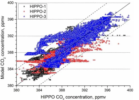
concentration. Modeled HIPPO-1’s precision successively exceeds 2 and 3, inferring the simulation results with the relevant either seasonal changes or data quality.

The simulation results of CO2concentration time-varying for HIPPO-1 using the

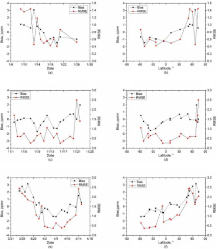
stan-dard model display good performance and weak dispersion of concentrations. The val-idation results (Fig. 2a) show that approximately 69.2 % of the absolute biases are

5

within 1 ppmv, approximately 92.3 % are within 2 ppmv, and only 7.7 % exceed 3 ppmv. Furthermore, as shown by the root-mean-square error (RMSE) with time, during most days in January the model values were stable compared with the observed values, apart from the first few days of the month. According to the simulation results of the HIPPO-1 observed and simulated latitude-varying CO₂ concentration data, the

com-10

parison values always underestimate the atmospheric XCO₂, and the di_fferences are all within 1.5 ppmv in the Southern Hemisphere, and vice versa in the Northern Hemi-sphere with 85.8 % of the differences under 1.1 ppmv. Figure 2b shows that the larger biases usually occur in the Northern Hemisphere high latitudes. The RMSE also re-flects the instability of the simulated values in the Northern Hemisphere high latitudes.

15

For HIPPO-2 data from 2 to 22 November 2009,the absolute biases of observed and simulated time-varying are all within 2 ppmv, and 77.8 % of the di_fferences are less than 1 ppmv (Fig. 2c). Approximately 5/6 of the data over the month show comparative stability. Similarly with HIPPO-1, the simulation results are always underestimates in the Southern Hemisphere and overestimates in the Northern Hemisphere. As shown

20

in Fig. 2d, the complete simulation displays good performance, apart from one day in the Northern Hemisphere high latitudes. In the same manner, the RMSE shows good stability in the Southern Hemisphere, in particular for the low-to mid-latitudes of the Southern Hemisphere. The model also simulates well in the Northern Hemisphere, especially from 45 to 70◦_N.

25

(11)

abso-ACPD

15, 6745–6770, 2015

Simulating CO2

C. Song et al.

Title Page

Tables Figures

◭ ◮

Back Close

Full Screen / Esc

Discussion

P

a

per

|

Discussion

P

a

per

|

Discussion

P

a

per

|

Discussion

P

a

per

|

lute biases were less than 1 ppmv, which suggests relatively good performance by the model simulation. As shown by the RMSE, the data for the last days in March were not stable. However, 81.8 % of the data in April showed comparatively good stability. The absolute biases are all under 1.5 ppmv in the Southern Hemisphere, and are also within 2 ppmv for the low- and mid-latitudes of the Northern Hemisphere (Fig. 2f). However,

5

a relatively large difference occurs at the Northern Hemisphere high latitudes, at one point exceeding 3 ppmv. Furthermore, the RMSE become greater with latitude from the Southern to Northern Hemisphere, inferring the simulation results are increasingly unstable with increasing latitude.

3.2 Validation of CO2vertical profiles 10

The GV flight plan performed 787 vertical ascents/descents from the ocean/ice sur-face/land surface to the tropopause. Two maximum altitude ascents were planned per flight to the tropopause/LS; one in the first half and the other in the second half of the research flight. In between, several vertical profiles from below the PBL to the mid-troposphere (1000–28 000 ft) were flown. Profiles were flown approximately every 2.2◦

15

of latitude with 4.4◦ _{between consecutive near-surface or high-altitude samples. Rate} of climb and descent was 1500 ft min−1 _{(457 m min}−1_{). During these profiles, the GV} averaged a ground speed of approximately 175 m s−1_{, or 10 km min}−1_.

Most of a flight was conducted below the international Reduced Vertical Separation Minimum (RVSM), usually 29 000 ft or 8850 m, to allow the GV to descend and climb

20

constantly to collect data at di_fferent altitudes throughout the troposphere. All flight plans were subject to modifications depending on local atmospheric conditions and approval by air traffic control. Most profiles extended from approximately 300 to 8500 m altitude, constrained by air tra_ffic, but significant profiling extended above approximately 14 km.

25

(12)

ACPD

15, 6745–6770, 2015

Simulating CO2

C. Song et al.

Title Page

Tables Figures

◭ ◮

Back Close

Full Screen / Esc

Discussion

P

a

per

|

Discussion

P

a

per

|

Discussion

P

a

per

|

Discussion

P

a

per

|

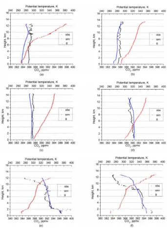
aerosol measurements from Mission 1 to 3. For each mission, several hundred vertical profiles were produced. We have only selected the vertical profiles from near-surface to LS to compare the simulations using the standard model with observations. Each mission can be divided into six parts for analysis; the low-, mid- and high-latitudes in the Southern and Northern Hemispheres, respectively.

5

For HIPPO-1, the total simulation value is always less than the observation value in the Southern Hemisphere and vice versa in the Northern Hemisphere. The bias is less than 2 ppmv for the entire profile from the near-surface to the LS; however, it increases from 2 to 4 ppmv above 10 km covering the Northern Hemisphere high latitudes.

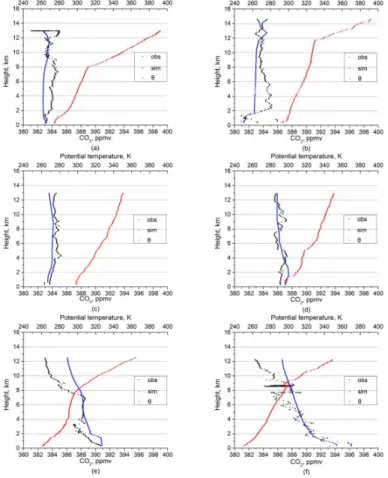
Figure 3 shows the comparison of simulation results and observations for data from

10

the near-surface to the LS in the low-, mid- and high- latitude. In the low-latitudes, as shown by Fig. 3c and d, the simulation performed very well compared with obser-vations. With the exception of the biases of approximately 2 ppmv in the tropopause in Fig. 3d, the biases are all within 1 ppmv. In the mid- and high-latitudes, it is di_ff er-ent in both hemispheres. In the Southern Hemisphere, the majority biases are within

15

2 ppmv but the LS zone in Fig. 3a and 2 to 6 km region in Fig. 3b. In the Northern Hemisphere (Fig. 3e and f), the simulated vertical profiles show good performances, apart from UTLS, and the biases are less than 2 ppmv. Some large biases occurred in the UTLS exceeding 4 ppmv when the potential temperature gradient increased rapidly with height.

20

HIPPO-2 data showed overall similarity with HIPPO-1 data based on the distribution of positive and negative bias. However, an anomaly occurred at approximately −60◦ and 75◦ _{latitude, showing positive and negative biases, respectively, some exceeding} 6 ppmv. Figure 4a is the vertical profile of the Southern Hemisphere high latitudes, which clearly shows that the simulation matches well with the observations from the

25

(13)

ACPD

15, 6745–6770, 2015

Simulating CO2

C. Song et al.

Title Page

Tables Figures

◭ ◮

Back Close

Full Screen / Esc

Discussion

P

a

per

|

Discussion

P

a

per

|

Discussion

P

a

per

|

Discussion

P

a

per

|

performance. For the mid-latitudes of the Northern Hemisphere, Fig. 4e shows rela-tively good simulation performance. However, as shown in Fig. 4f, the high latitudes did not perform well in the near-surface or the low- and mid-troposphere. Compared with observations, the simulation profiles do not appear to reflect the original shape.

As shown by HIPPO-3 data the biases increase abruptly with flight height for the

5

mid- to high-latitudes of the Northern Hemisphere with values reaching 7 ppmv. In the high-latitudes of the Southern Hemisphere (Fig. 5a) the simulation underestimates the observations, and the absolute biases are isostatic from the near-surface to the LS, which are less than 3 ppmv. The Southern Hemisphere low latitudes (Fig. 5c) indicate good performance of the simulations, where all the biases are less than 1 ppmv. In the

10

Northern Hemisphere low latitudes (Fig. 5d), the entire simulation appears to match well with observations. However, some locations do not reproduce the precise shape through the entire height. For the mid- to high- northern latitudes (Fig. 5e and f), the simulations performed relatively well from the near-surface to the UT. Larger bias in simulations is found in the winter lower stratosphere in the northern high-latitudes. The

15

problem appears because between tropopause and 350 K level model uses vertical wind provided by reanalysis instead of using radiative heating rate, which is more ac-curate in stratosphere. The positive bias can reach level of 4 ppm for CO2. This problem

only affects simulations for observation made in lower stratosphere in high latitudes in cold season when the tropopause level is low. However the number of in-situ

observa-20

tions made in this altitude is very limited. The satellite observations of the total column such as GOSAT are also reduced considerably in high latitudes in cold season (Yoshida et al., 2013). Thus this lower stratosphere bias is not likely to deteriorate the transport model performance in the inverse modeling applications.

4 Conclusions

25

(14)

ACPD

15, 6745–6770, 2015

Simulating CO2

C. Song et al.

Title Page

Tables Figures

◭ ◮

Back Close

Full Screen / Esc

Discussion

P

a

per

|

Discussion

P

a

per

|

Discussion

P

a

per

|

Discussion

P

a

per

|

and aerosol data from Missions 1 to 3, which span three different seasons (autumn, winter and spring). The results show that the model somewhat underestimates CO2in

the Southern Hemisphere and overestimates it in the Northern Hemisphere for these three missions. However, the model was able to reproduce the seasonal and inter-annual variability of XCO2 with RMS bias across all profiles with a level of 0.9 ppmv. 5

The model performed well from the near-surface layer to the top of the troposphere, apart from the lower stratosphere the high latitude regions, in particular, in the North-ern Hemisphere in spring, where large biases would often appear. The smaller bias of HIPPO-1 in January compared with HIPPO-3 in March and April arises from sea-sonal changes in meteorology and using the simplified fluxes, as mentioned in Patra

10

et al. (2008).

The accuracy of these calculations will increase with the adaptation of the mass-balanced reanalysis data (MERRA, Bosilovich et al., 2008). Demand for global high-resolution fields of CO₂ and other greenhouse gases will also increase because of their use as a priori information in retrieval algorithms of observation instruments, such

15

as the AIRS satellite (e.g., Strow and Hannon, 2008) and GOSAT (e.g., Yokota et al., 2009), and regional inverse modeling studies (Thompson et al., 2014).

Acknowledgements. The authors acknowledge the HIPPO data set available from CDIAC

(ORNL). This project was supported by the National Basic Research Program of China (No. 2010CB951603). The computation was supported by the High Performance Computer

20

Center of East China Normal University. We thank the team members of the Biogeochemical Cycle Modeling and Analysis Section of National Institute for Environment Studies, Tsukuba, Japan for providing expert advice and assistance. The GOSAT Level 4 data made available by GOSAT project (http://www.gosat.nies.go.jp/index_e.html).

References

25

(15)

ACPD

15, 6745–6770, 2015

Simulating CO2

C. Song et al.

Title Page

Tables Figures

◭ ◮

Back Close

Full Screen / Esc

Discussion

P

a

per

|

Discussion

P

a

per

|

Discussion

P

a

per

|

Discussion

P

a

per

|

intercomparison: impact of transport model errors on the interannual variability of regional CO₂fluxes 1988–2003, Global Biogeochem. Cy., 20, GB1002, doi:10.1029/2004GB002439, 2006.

Belikov, D., Maksyutov, S., Miyasaka, T., Saeki, T., Zhuravlev, R., and Kiryushov, B.: Mass-conserving tracer transport modelling on a reduced latitude-longitude grid with NIES-TM,

5

Geosci. Model Dev., 4, 207–222, doi:10.5194/gmd-4-207-2011, 2011.

Belikov, D. A., Maksyutov, S., Sherlock, V., Aoki, S., Deutscher, N. M., Dohe, S., Griffith, D., Kyro, E., Morino, I., Nakazawa, T., Notholt, J., Rettinger, M., Schneider, M., Sussmann, R., Toon, G. C., Wennberg, P. O., and Wunch, D.: Simulations of column-averaged CO₂and CH₄ using the NIES TM with a hybrid sigma-isentropic (σ–θ) vertical coordinate, Atmos. Chem.

10

Phys., 13, 1713–1732, doi:10.5194/acp-13-1713-2013, 2013.

Bolin, B. and Keeling, C. D.: Large scale atmospheric mixing as deduced from seasonal and meridional variations of the atmospheric carbon dioxide, J. Geophys. Res., 68, 3899–3920, 1963.

Bosilovich, M. G., Chen, J., Robertson, F. R., and Adler, R. F.: Evaluation of global precipitation

15

in reanalysis, J. Appl. Meteorol. Clim., 47, 2279–2299, doi:10.1175/2008JAMC1921.1, 2008. Bregman, B., Meijer, E., and Scheele, R.: Key aspects of stratospheric tracer modeling

us-ing assimilated winds, Atmos. Chem. Phys., 6, 4529–4543, doi:10.5194/acp-6-4529-2006, 2006.

Ciais, P., Sabine C., Bala G., Bopp L., Brovkin V., Canadell J., Chhabra A., DeFries R., Galloway

20

J., Heimann M., Jones C., Le Quéré, C., Myneni R. B., Piao S., and Thornton P.: Carbon and Other Biogeochemical Cycles, in: Climate Change 2013: The Physical Science Basis. Contribution of Working Group I to the Fifth Assessment Report of the Intergovernmental Panel on Climate Change, edited by: Stocker, T. F., Qin, D., Plattner, G.-K., Tignor, M., Allen, S. K., Boschung, J., Nauels, A., Xia, Y., Bex, V., and Midgley, P. M., Cambridge University

25

Press, Cambridge, United Kingdom and New York, NY, USA, 2013.

Dee, D. P. and Uppala, S.: Variational bias correction of satelliteradiance data in the ERA-Interim reanalysis, Q. J. Roy. Meteor. Soc., 135, 1830–1841, 2009.

Denning, A. S., Randall, D. A., Collatz, G. J., and Sellers, P. J.: Simulations of terrestrial carbon metabolism and atmospheric CO₂in a general circulation model. II. Simulated CO₂

concen-30

trations, Tellus B, 48, 543–567, doi:10.1034/j.1600-0889.1996.t01-1-00010.x, 1996.

(16)

ACPD

15, 6745–6770, 2015

Simulating CO2

C. Song et al.

Title Page

Tables Figures

◭ ◮

Back Close

Full Screen / Esc

Discussion

P

a

per

|

Discussion

P

a

per

|

Discussion

P

a

per

|

Discussion

P

a

per

|

Three-dimensional transport and concentration of SF6: a model intercomparison study (TransCom2), Tellus B, 51, 266–297, 1999.

Douglass, A. R., Prather, M. J., Hall, T. M., Strahan, S. E., Rasch, P. J., Sparling, L. C., Coy, L., and Rodriguez, J. M.: Choosing meteorological input for the global modeling initiative as-sessment of high-speed aircraft, J. Geophys. Res., 104, 27545–27564, 1999.

5

GLOBALVIEW-CO₂: Cooperative Atmospheric Data Integration Project–Carbon Dioxide, CD-ROM, NOAA ESRL, Boulder, Colorado, 2010.

Gurney, K. R., Law, R. M., Denning, A. S., Rayner, P. J., Pak, B. C., Baker, D., Bousquet, P., Bruhwiler, L., Chen, Y. H., Ciais, P., Fung, I. Y., Heimann, M., John, J., Maki, T., Maksyutov, S., Peylin, P., Prather, M., and Taguchi, S.: Transcom 3 inversion intercomparison: model mean

10

results for the estimation of seasonal carbon sources and sinks, Global Biogeochem. Cy., 18, GB1010, doi:10.1029/2003GB002111, 2004.

Hack, J. J., Boville, B. A., Briegleb, B. P., Kiehl, J. T., Rasch, P. J., and Williamson, D. L.: Description of the NCAR Community Climate Model (CCM2), NCAR/TN-382, 108, Climate and Global Dynamics Division, NCAR, Boulder, Colorado, USA, 1993.

15

Hall, T. M., Waugh, D. W., Boering, K. A., and Plumb, R. A.: Evaluation of transport in strato-spheric models, J. Geophys. Res., 104, 18815–18839, 1999.

Hein, R., Crutzen, P. J., and Heimann, M.: An inverse modeling approach to investigate the global atmospheric methane cycle, Global Biogeochem. Cy., 11, 43–76, 1997.

Jacob, D., Prather, M. J., Rasch, P. J., Shea, R.-L., Balkanski, Y. J., Beagley, S. R.,

20

Bergmann, D. J., Blackshear, W. T., Brown, M., Chiba, M., Chipperfield, M. P., de Grand-pré, J., Dignon, J. E., Feichter, J., Genthon, C., Grose, W. L., Kasibhatla, P. S., Köhler, I., Kritz, M. A., Law, K., Penner, J. E., Ramonet, M., Reeves, C. E., Rotman, D. A., Stock-well, D. Z., Van Velthoven, P. F. J., Verver, G., Wild, O., Yang, H., and Zimmermann, P.: Evaluation and intercomparison of global transport models using222Rn and other short-lived

25

tracers, J. Geophys. Res., 102, 5953–5970, 1997.

Jöckel, P., von Kuhlmann, R., Lawrence, M. G., Steil, B., Brenninkmeijer, C. A. M., Crutzen, P. J., Rasch, P. J., and Eaton, B.: On a fundamental problem in implementing flux-form advection schemes for tracer transport in 3-dimensional general circulation and chemistry transport models, Q. J. Roy. Meteor. Soc., 127, 1035–1052, 2001.

30

(17)

ACPD

15, 6745–6770, 2015

Simulating CO2

C. Song et al.

Title Page

Tables Figures

◭ ◮

Back Close

Full Screen / Esc

Discussion

P

a

per

|

Discussion

P

a

per

|

Discussion

P

a

per

|

Discussion

P

a

per

|

Law, R. M., Peters, W., Rödenbeck, C., Aulagnier, C., Baker, I., Bergmann, D. J., Bousquet, P., Brandt, J., Bruhwiler, L., Cameron-Smith, P. J., Christensen, J. H., Delage, F., Denning, A. S., Fan, S.-M., Geels, C., Houweling, S., Imasu, R., Karstens, U., Kawa, S. R., Kleist, J., Krol, M., Lin, S.-J., Lokupitiya, R., Maki, T., Maksyutov, S., Niwa, Y., Onishi, R., Parazoo, N., Pa-tra, P. K., Pieterse, G., Rivier, L., Satoh, M., Serrar, S., Taguchi, S., Takigawa, M.,

Vau-5

tard, R., Vermeulen, A. T., and Zhu, Z.: Trans Commodel simulations of hourly atmospheric CO₂: experimental overview and diurnal cycle results for 2002, Global Biogeochem. Cy., 22, GB3009, doi:10.1029/2007GB003050, 2008.

Mahowald, N. M., Plumb, R. A., Rasch, P. J., del Corral, J., and Sassi, F.: Stratospheric transport in a three-dimensional isentropic coordinate model, J. Geophys. Res., 107, 4254,

10

doi:10.1029/2001JD001313, 2002.

Maksyutov, S., Patra, P. K., Onishi, R., Saeki, T., and Nakazawa, T.: NIES/FRCGC global at-mospheric tracer transport model: description, validation, and surface sources and sinks inversion, Journal of the Earth Simulator, 9, 3–18, 2008.

Monge-Sanz, B. M., Chipperfield, M. P., Simmons, A. J., and Uppala, S. M.: Mean age of air

15

and transport in a CTM: comparison of different ECMWF analyses, Geophys. Res. Lett., 34, L04801, doi:10.1029/2006GL028515, 2007.

Niwa, Y., Patra, P. K., Sawa, Y., Machida, T., Matsueda, H., Belikov, D., Maki, T., Ikegami, M., Imasu, R., Maksyutov, S., Oda, T., Satoh, M., and Takigawa, M.: Three-dimensional vari-ations of atmospheric CO₂: aircraft measurements and multi-transport model simulations,

20

Atmos. Chem. Phys., 11, 13359–13375, doi:10.5194/acp-11-13359-2011, 2011.

Onogi, K., Tsutsui, J., Koide, H., Sakamoto, M., Kobayashi, S., Hatsushika, H., Matsumoto, T., Yamazaki, N., Kamahori, H., Takahashi, K., Kadokura, S., Wada, K., Kato, K., Oyama, R., Ose, T., Mannoji, N., and Taira, R.: The JRA-25 reanalysis, J. Meteorol. Soc. Jap., 85, 369– 432, 2007.

25

Parker, R., Boesch, H., Cogan, A., Fraser, A., Feng, L., Palmer, P. I., Messerschmidt, J., Deutscher, N., Griffith, D. W. T., Notholt, J., Wennberg, P. O., and Wunch, D.: Methane observations from the Greenhouse Gases Observing SATellite: comparison to ground based TCCON data and model calculations, Geophys. Res. Lett., 38, L15807, doi:10.1029/2011GL047871, 2011.

30

(18)

ACPD

15, 6745–6770, 2015

Simulating CO2

C. Song et al.

Title Page

Tables Figures

◭ ◮

Back Close

Full Screen / Esc

Discussion

P

a

per

|

Discussion

P

a

per

|

Discussion

P

a

per

|

Discussion

P

a

per

|

Sensitivity of optimal extension of observation networks to the model transport, Tellus B, 55, 498–511, 2003a.

Patra, P. K., Maksyutov, S., Sasano, Y., Nakajima, H., Inoue, G., and Nakazawa, T.: An evalu-ation of CO₂ observations with Solar Occultation FTS for Inclined-Orbit Satellite sensor for surface source inversion, J. Geophys. Res., 108, 4759, doi:10.1029/2003JD003661, 2003b.

5

Patra, P. K., Peters, W., Rödenbeck, C., Aulagnier, C., Baker, I., Bergmann, D. J., Bousquet, P., Brandt, J., Bruhwiler, L., Cameron-Smith, P. J., Christensen, J. H., Delage, F., Denning, A. S., Fan, S.-M., Geels, C., Houweling, S., Imasu, R., Karstens, U., Kawa, S. R., Kleist, J., Krol, M., Law, R. M., Lin, S.-J., Lokupitiya, R., Maki, T., Maksyutov, S., Niwa, Y., Onishi, R., Para-zoo, N., Pieterse, G., Rivier, L., Satoh, M., Serrar, S., Taguchi, S., Takigawa, M., Vautard, R.,

10

Vermeulen, A. T., and Zhu, Z.: TransCom model simulations of hourly atmospheric CO₂: analysis of synoptic-scale variations for the period 2002–2003, Global Biogeochem. Cy., 22, GB4013, doi:10.1029/2007GB003081, 2008.

Rasch, P. J., Boville, B. A., and Brasseur, G. P.: A three dimensional general circulation model with coupled chemistry for the middle atmosphere, J. Geophys. Res., 100, 9041–9071, 1995.

15

Raupach, M. R., Marland, G., Ciais, P., Le Quere, C., Canadell, J. G., Klepper, G., and Field, C. B.: Global and regional drivers of accelerating CO₂ emissions, P. Natl. Acad. Sci. USA, 104, 288–293, doi:10.1073/pnas.0700609104, 2007.

Rayner, P. J. and O’Brien, D. M.: The utility of remotely sensed CO₂ concentration data in surface inversion, Geophys. Res. Lett., 28, 175–178, 2001.

20

Rayner, P. J., Entiing, I. G., Francey, R. J., and Langenfelds, R.: Reconstructing the recent carbon cycle from atmospheric CO₂,δ13C and O₂/N₂observations, Tellus B, 51, 213–232, 1999.

Schoeberl, M. R., Douglass, A. R., Zhu, Z., and Pawson, S.: Acomparison of the lower strato-spheric age spectra derived from a general circulation model and two data assimilation

sys-25

tems, J. Geophys. Res., 108, 4113, doi:10.1029/2002JD002652, 2003.

Scholes, R. J., Monteiro, P. M. S., Sabine, C. L., and Canadell, J. G.: Systematic long-term observations of the global carbon cycle, Trends Ecol. Evol., 24, 427–430, doi:10.1016/j.tree.2009.03.006, 2009.

Stohl, A., Cooper, O., and James, P.: A cautionary note on the use of meteorological analysis

30

(19)

ACPD

15, 6745–6770, 2015

Simulating CO2

C. Song et al.

Title Page

Tables Figures

◭ ◮

Back Close

Full Screen / Esc

Discussion

P

a

per

|

Discussion

P

a

per

|

Discussion

P

a

per

|

Discussion

P

a

per

|

Strow, L. L. and Hannon, S. E.: A 4-year zonal climatology of lower tropospheric CO₂ de-rived from ocean-only Atmospheric Infrared Sounder observations, J. Geophys. Res., 113, D18302, doi:10.1029/2007JD009713, 2008.

Tans, P., Fung, I., and Takahashi, T.: Observational constraints of the global atmospheric CO₂ budget, Science, 247, 1431–1438, 1990.

5

Thompson, R. L., Ishijima, K., Saikawa, E., Corazza, M., Karstens, U., Patra, P. K., Berga-maschi, P., Chevallier, F., Dlugokencky, E., Prinn, R. G., Weiss, R. F., O’Doherty, S., Fraser, P. J., Steele, L. P., Krummel, P. B., Vermeulen, A., Tohjima, Y., Jordan, A., Haszpra, L., Steinbacher, M., Van der Laan, S., Aalto, T., Meinhardt, F., Popa, M. E., Moncrieff, J., and Bousquet, P.: TransCom N₂O model inter-comparison – Part 2: Atmospheric inversion

es-10

timates of N₂O emissions, Atmos. Chem. Phys., 14, 6177–6194, doi:10.5194/acp-14-6177-2014, 2014.

Waugh, D. W. and T. M. Hall, Age of stratospheric air: Theory, observations, and models, Rev. Geophys., 40, 1010, doi:10.1029/2000RG000101, 2002.

Wunch, D., Toon, G., Blavier, J.-F. L., Washenfelder, R. A., Notholt, J., Connor, B. J.,

Grif-15

fith, D. W. T., Sherlock, V., and Wennberg, P. O.: The Total Carbon Column Observing Net-work (TCCON), Philos. T. R. Soc. A, 369, 2087–2112, doi:10.1098/rsta.2010.0240, 2011. Yang, Z., Washenfelder, R. A., Keppel-Aleks, G., Krakauer, N. Y., Randerson, J. T., Tans, P. P.,

Sweeney, C., and Wennberg, P. O.: New constraints on Northern Hemisphere growing sea-son net flux P, Geophys. Res. Lett., 34, 1–6, doi:10.1029/2007GL029742, 2007.

20

Yokota, T., Yoshida, Y., Eguchi, N., Ota, Y., Tanaka, T., Watanabe, H., and Maksyutov, S.: Global concentrations of CO₂ and CH₄ retrieved from GOSAT: first preliminary results, SOLA, 5, 160–163, doi:10.2151/sola.2009-041, 2009.

Yoshida, Y., Kikuchi, N., Morino, I., Uchino, O., Oshchepkov, S., Bril, A., Saeki, T., Schutgens, N., Toon, G. C., Wunch, D., Roehl, C. M., Wennberg, P. O., Griffith, D. W. T., Deutscher, N. M.,

25

Warneke, T., Notholt, J., Robinson, J., Sherlock, V., Connor, B., Rettinger, M., Sussmann, R., Ahonen, P., Heikkinen, P., Kyrö, E., Mendonca, J., Strong, K., Hase, F., Dohe, S., and Yokota, T.: Improvement of the retrieval algorithm for GOSAT SWIR XCO₂ and XCH₄ and their validation using TCCON data, Atmos. Meas. Tech., 6, 1533–1547, doi:10.5194/amt-6-1533-2013, 2013.

(20)

ACPD

15, 6745–6770, 2015

Simulating CO2

C. Song et al.

Title Page

Tables Figures

◭ ◮

Back Close

Full Screen / Esc

Discussion

P

a

per

|

Discussion

P

a

per

|

Discussion

P

a

per

|

Discussion

P

a

per

|

Table 1.Vertical grid levels of the NIES TM model.

H, km σ=P/Ps ≈∆, m ξ(σ–θgrid levels), K Number of levels

Near-surface layer 0–2 1.0–0.795 250 – 8

Free troposphere 2–12 0.795–0.195 1000 –, 330, 350, 10 Upper troposphere and stratosphere 12–40 0.195–0.003 1000 365, 380, 400, 415,

435, 455, 475, 500, 14

2000 –

545,

590, 665, 850, 1325, 1710

Total levels: 32

H, height.

P, atmospheric pressure. Ps, surface atmospheric pressure.

∆, vertical integral step.

(21)

ACPD

15, 6745–6770, 2015

Simulating CO2

C. Song et al.

Title Page

Tables Figures

◭ ◮

Back Close

Full Screen / Esc

Discussion

P

a

per

|

Discussion

P

a

per

|

Discussion

P

a

per

|

Discussion

P

a

per

|

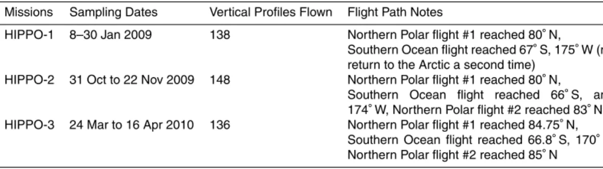
Table 2.Temporal and spatial (horizontal) coverage of HIPPO mission flights.

Missions Sampling Dates Vertical Profiles Flown Flight Path Notes

HIPPO-1 8–30 Jan 2009 138 Northern Polar flight #1 reached 80◦_N,

Southern Ocean flight reached 67◦

S, 175◦

W (no return to the Arctic a second time)

HIPPO-2 31 Oct to 22 Nov 2009 148 Northern Polar flight #1 reached 80◦_N,

Southern Ocean flight reached 66◦_{S, and}

174◦_{W, Northern Polar flight #2 reached 83}◦_N

HIPPO-3 24 Mar to 16 Apr 2010 136 Northern Polar flight #1 reached 84.75◦_N,

Southern Ocean flight reached 66.8◦_{S, 170}◦_E,

Northern Polar flight #2 reached 85◦

(22)

ACPD

15, 6745–6770, 2015

Simulating CO2

C. Song et al.

Title Page

Tables Figures

◭ ◮

Back Close

Full Screen / Esc

Discussion

P

a

per

|

Discussion

P

a

per

|

Discussion

P

a

per

|

Discussion

P

a

per

|

(23)

ACPD

15, 6745–6770, 2015

Simulating CO2

C. Song et al.

Title Page

Tables Figures

◭ ◮

Back Close

Full Screen / Esc

Discussion

P

a

per

|

Discussion

P

a

per

|

Discussion

P

a

per

|

Discussion

P

a

per

|

Figure 2. Bias (simulation-observation, black square) and RMSE (red circle) of time-((a) HIPPO-1, (c) HIPPO-2, (e) HIPPO-3) and latitude-varying ((b) HIPPO-1, (d) HIPPO-2,

(24)

ACPD

15, 6745–6770, 2015

Simulating CO2

C. Song et al.

Title Page

Tables Figures

◭ ◮

Back Close

Full Screen / Esc

Discussion

P

a

per

|

Discussion

P

a

per

|

Discussion

P

a

per

|

Discussion

P

a

per

|

(25)

ACPD

15, 6745–6770, 2015

Simulating CO2

C. Song et al.

Title Page

Tables Figures

◭ ◮

Back Close

Full Screen / Esc

Discussion

P

a

per

|

Discussion

P

a

per

|

Discussion

P

a

per

|

Discussion

P

a

per

|

(26)

ACPD

15, 6745–6770, 2015

Simulating CO2

C. Song et al.

Title Page

Tables Figures

◭ ◮

Back Close

Full Screen / Esc

Discussion

P

a

per

|

Discussion

P

a

per

|

Discussion

P

a

per

|

Discussion

P

a

per

|