Ann. Geophys., 27, 4229–4238, 2009 www.ann-geophys.net/27/4229/2009/
© Author(s) 2009. This work is distributed under the Creative Commons Attribution 3.0 License.
Annales
Geophysicae
Observational evidence for the plausible linkage of Equatorial
Electrojet (EEJ) electric field variations with the post sunset
F-region electrodynamics
V. Sreeja, C. V. Devasia, Sudha Ravindran, and Tarun Kumar Pant
Space Physics Laboratory, Vikram Sarabhai Space Centre, Trivandrum 695022, India
Received: 3 April 2009 – Revised: 12 October 2009 – Accepted: 30 October 2009 – Published: 10 November 2009
Abstract. The paper is based on a detailed observational study of the Equatorial Spread F (ESF) events on geomag-netically quiet (Ap≤20) days of the solar maximum (2001), moderate (2004) and minimum (2006) years using the iono-grams and magnetoiono-grams from the magnetic equatorial loca-tion of Trivandrum (8.5◦N; 77◦E; dip lat∼0.5◦N) in India. The study brings out some interesting aspects of the day-time Equatorial Electrojet (EEJ) related electric field varia-tions and the post sunset F-region electrodynamics governing the nature of seasonal characteristics of the ESF phenomena during these years. The observed results seem to indicate a plausible linkage of daytime EEJ related electric field varia-tions with pre-reversal enhancement which in turn is related to the occurrence of ESF. These electric field variations are shown to be better represented through a parameter, termed as “E”, in the context of possible coupling between the E-and F-regions of the ionosphere. The observed similarities in the gross features of the variations in the parameter “E” and the F-region vertical drift (Vz) point towards the potential us-age of the EEJ related parameter “E” as an useful index for the assessment ofVzprior to the occurrence of ESF. Keywords. Ionosphere (Electric fields and currents; Equa-torial ionosphere; Ionospheric irregularities)
1 Introduction
The electrodynamics of the equatorial ionospheric E- and F-regions is essentially controlled by the electric fields gen-erated by the movement of the electrically conducting up-per atmosphere across the Earth’s magnetic field through neutral wind forcings. Major phenomena of the equato-rial ionosphere are mostly associated with the generation of
Correspondence to: V. Sreeja
Equatorial Electrojet (EEJ), which is a narrow band of en-hanced eastward current flowing in the 100–120 km altitude region i.e. E-region within±3◦latitude of the dip equator in the morning, and the subsequent development of the Equa-torial Ionization Anomaly (EIA), also known as Appleton Anomaly, in the F-region.
After sunrise with the build up of the EEJ, the east-west component of its electric field E (which has its origin in the global dynamo field) gets mapped to the F-region alti-tudes along the highly conducting geomagnetic field lines. In the F-region, the electric fieldEcauses the verticalE×B plasma drift through the interaction with the north-south component of the Earth’s magnetic field (B) and causes the development of EIA. The EEJ grows in strength reaching a maximum around local noon followed by its gradual decay to a low value at around sunset, as indicated by the EEJ induced ground magnetic field (B) variations.
The F-region plasma that is uplifted over the dip equator, by the process of the verticalE×Bplasma drift (also called the plasma fountain process), diffuses along the Earth’s mag-netic field lines resulting in depletion (accumulation) of plasma around the dip equator (away from the equator) pro-ducing a double humped latitudinal distribution, known as EIA, on either side of the magnetic equator at±15–20◦dip latitude. The EIA forms generally at around 09:00 LT with the crests close to the dip equator to start with, and gains in strength (with both poleward movement and intensification of crests) in the afternoon period (Sastri, 1990). A one-to-one correlation between the strength of the EIA and the time integrated strength of the EEJ has been observed, confirm-ing that the drivconfirm-ing force for both the EIA and the EEJ is the same (Dunford, 1967; Rastogi and Rajaram, 1971; Rush and Richmond, 1973; Raghavarao et al., 1978).
4230 V. Sreeja et al.: Observational evidence for the plausible linkage of EEJ discussed the large day-to-day variability in the F-region
ver-tical drift velocities as measured by the Jicamarca Incoherent Scatter radar. Anderson et al. (2002) established a quantita-tive relationship between the verticalE×Bdrift velocity in the ionospheric F-region and the daytime strength of the EEJ in the South American (west coast) longitude sector.
It is well known that the F-region plasma drift reverses from upward to downward after sunset. However, just before the reversal, there is a clear cut post sunset enhancement in the verticalE×Bdrift associated with the activation of the F-region dynamo in the evening hours (Rishbeth, 1981; Ec-cles, 1998). This is called the post sunset or the pre-reversal enhancement (PRE) of the F-region zonal electric field. The PRE is basically responsible for the large uplift of the F-layer and the evening time resurgence of the EIA. The exact mech-anism for the post sunset F-layer uplift i.e. whether it is due to the F-region dynamo electric fields getting freed from the field line E-region loading effect (Farley et al., 1986) or due to the irrotational nature of the electric field at the sunset ter-minator manifesting itself as an enhanced zonal wind (Rish-beth, 1981) or due to the evening EEJ (Haerendel and Ec-cles, 1992) is still not fully understood. Recently, Kelley et al. (2009) considered the above three competing mechanisms that exist for the PRE, in the light of the penetration of a large electric field of interplanetary origin. Their study suggests that the normal PRE must be created by the Haerendel and Eccles (1992) mechanism, in which the EEJ partially closes in the post sunset F-region, and that the other two mecha-nisms are secondary. However, whatever be the mechanism, the fact is that during the sunset hours, the F-region is up-lifted to higher altitudes due to the enhanced zonal electric field, the magnitude of which exhibits large day-to-day vari-ability. At higher altitudes, conditions are conducive for the triggering of the plasma instability responsible for Equato-rial Spread F (ESF)/plasma bubble irregularity events in the nighttime F-region.
The plasma irregularities in the nighttime equatorial F-region manifest in the form of diffuse echoes in the iono-grams and are known as ESF. By a careful analysis of ground based ionospheric data, a close linkage between EIA and ESF was shown by Raghavarao et al. (1988), Alex et al. (1989) and Jayachandran et al. (1997). The basic mecha-nism responsible for the generation of ESF is the Collisional Rayleigh-Taylor (CRT) plasma instability. After local sun-set, the base of the F-region gets lifted up because of two factors (i) the recombination of molecular ions in the lower F-region and (ii) the electrodynamical lifting of the F-region (Rishbeth, 1981; Eccles, 1998). The lifting of the F-region to 300 km and beyond is generally considered to be a necessary condition for the triggering of R-T instability, though may not be sufficient (Rishbeth, 1981). The PRE has a strong control on the height rise of the evening equatorial F layer by generating steep vertical gradients in the electron density profile and as a consequence on the occurrence of ESF. Fejer et al. (1999) have studied the effects ofVz on the
genera-tion and evolugenera-tion of ESF, while Hysell (2000) has given an overview of plasma irregularities causing ESF.
The occurrence of ESF varies from day-to-day with sea-son, geographical location and also with solar and geomag-netic activity. These aspects of ESF have been studied extensively over the past several years (Chandra and Ras-togi, 1970; Woodman and LaHoz, 1976; Fejer and Kel-ley, 1980; Maruyama and Matuura, 1984; Aarons, 1993; Hysell and Burcham, 2002, and the references therein). Maruyama (1988) studied the effects of the meridional winds and showed that a poleward wind would inhibit ESF by push-ing the ionization along the field lines to the E-region. The increased conductivity in the E-region would oppose the up-liftment of the base of the F-region to greater heights by load-ing the F-region dynamo. However, the polarity (equator-ward/poleward) and magnitude of the meridional winds have been shown to play a significant role only when the maxi-mum bottom height of the post sunset F-layer (h′F) is below a critical height. Above the critical height, the polarity of the winds was shown to be not having a direct control on the generation of ESF (Devasia et al., 2002).
While the aspect of the seasonal variation of ESF is rea-sonably understood (Abdu et al., 2000), the day-to-day and shorter term variabilities are not adequately understood be-cause of a lack of knowledge on the interdependent vari-abilities of the ambient E- and F-region parameters that control the ESF development. The presence of ESF ir-regularities can cause scintillations in VHF, UHF and even the microwave frequency range. These scintillations pro-duce disruptions of the communication and navigation links using satellites. Hence, understanding the variability of ESF occurrence and forecasting of this phenomenon are of practical importance. It is the background electrodynamic and neutral dynamic conditions that basically dictate the occurrence/non-occurrence of ESF on a particular day. Ear-lier studies have tried to make an attempt to forecast the oc-currence of ESF (Raghavarao et al., 1988; Sridharan et al., 1994; Mendillo et al., 2001; Thampi et al., 2006, and the ref-erences therein). These studies imply that the background ionospheric and thermospheric conditions during the day-time play a very crucial role in the generation of ESF.
V. Sreeja et al.: Observational evidence for the plausible linkage of EEJ 4231 2 Data and methodology of analysis
The study is based on the analysis of ionograms and mag-netograms obtained at the magnetic equatorial location of Trivandrum (8.5◦N; 77◦E; dip lat ∼0.5◦N) in India dur-ing the solar maximum year of 2001, moderate activity year of 2004 and the minimum year of 2006. Information about the F-region parameters like foF2 (critical frequency of the F-layer) andh′F have been obtained from the quarter hourly ionograms available during all the magnetically quiet (Ap≤20) days of these years. We have adopted the com-monly used method of using the information on the evening timeh′F variations to computedh′F /dtor equivalently the E×Bdrift for obtaining the PRE. The vertical drift velocity Vz (PRE) of the layer as given by,Vz=[d(h′F )/dt], should be close to the real F-region vertical plasma drifts for layer heights≥300 km (Bittencourt and Abdu, 1981; Batista et al., 1986), which usually is the case during evening hours for the solar maximum year. The F-region height rise due to chemi-cal losses is of the order of 5 m/s and is negligible when com-pared to large vertical drift velocities due to the PRE in the zonal electric field (Krishna Murthy et al., 1990; Basu et al., 1996). Another method for deriving the F-region drift has been evolved by using the information on the hmF2 values obtained from the electron density profile (Liu et al., 2004, and the references therein).
SinceE×Bdrift velocity generally reaches its maximum before the onset of ESF (Fejer et al., 1999; Whalen, 2002), the maximumE×B drift velocity (Vz)and its occurrence time during the post sunset hours have also been used as im-portant parameters in relation to the ESF onset time on each day. The time of the maximumVzcan be treated as the re-versal time of the upwardE×Bdrift.
Hourly values of the Earth’s magnetic field (1H) at Trivandrum and at Alibag (18.7◦N; 73◦E; dip lat∼13◦N), a location outside the electrojet region, published by Indian Institute of Geomagnetism (IIG), Mumbai (India) is used to characterize the strength of EEJ on each day as given by the relationship, (1HTIR−1HABG). However, Devasia et al. (2006) have shown that the hourly values of (1H) at Trivandrum (1HTIR)denotes the intensity/strength of EEJ over the magnetic equatorial location of Trivandrum and that the time variations of (1HTIR) i.e. {d1HTIR)/dt} during daytime is a proxy parameter for indicating the variations in the east-west electric field in EEJ. The maximum gradient of
{d1HTIR)/dt}denoted as{(d1HTIR)/dt)max}in the morn-ing hours is assumed to give an indirect estimate of the maxi-mum build up rate of the EEJ electric field. The above param-eters thus obtained on each of the ESF days have been used to examine the relationship/correspondence, if any, between the EEJ related variability and the occurrence of ESF through the inter-dependence between the development of EIA, strength and occurrence time ofVz.
3 Results and discussion
3.1 Nature of variation of E- and F-region parameters: growth and decay rates of the daytime EEJ strength
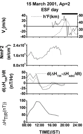
Figure 1a and b shows the temporal variations of the rele-vant E- and F-region parameters on a typical ESF (15 March 2001) and a non-ESF day (4 March 2001) during the period under study. The bottom panels of Fig. 1a and b give the day-time variations of1H over Trivandrum on the ESF day and the non-ESF day respectively. The second panel from bottom shows the time variations ofd(1HTIR)/dt and{d(1HTIR− 1HABG)/dt}. The variations of both {d(1HTIR)/dt} and
{d(1HTIR−1HABG)/dt}are “quite similar”, except for a small constant difference in their magnitudes. The third panel from bottom represents the variations in the NmF2 or equivalently in [foF2]2{proportional to the electron number density (N) corresponding to foF2}.
The temporal variations ofd(1HTIR)/dt and NmF2 show distinctly different pattern on the ESF and the non-ESF days, with considerable difference in the maximum values of d(1HTIR)/dtin the morning and afternoon hours. The max-imum values of{d(1HTIR)/dt}in the morning (i.e. usually around 09:30–10:30 IST) and afternoon hours (i.e. around 14:30–15:30 IST) gives respectively the maximum values of the growth and decay rates of the EEJ electric field. Their amplitudes (maximum values) as well as their time of occur-rence show variability on a day-to-day, monthly, seasonal as well as on solar activity level basis.
Other parameters of interest in the post sunset F-region are the variations inVzandh′F which are shown in the top panels of Fig. 1a and b. The presence of large value forVz andh′F in the post sunset hours preceding the ESF
occur-rence is the most important characteristic feature observed on the ESF day in comparison to the non-ESF day. The na-ture of variability of the maximum value of{d(1HTIR)/dt} is observed to have some sort of an association with the ESF occurrence. The present study is an attempt to inves-tigate their plausible linkage with the post sunset F-region behaviour during different seasons under the different solar activity conditions.
4232 V. Sreeja et al.: Observational evidence for the plausible linkage of EEJ Δ
Δ Δ Δ
Fig. 1a. Variations in1HTIR(bottom panel) along with the vari-ations in{d(1HTIR)/dt}and{d(1HABG−1HTIR)/dt}(second panel), NmF2=1.24e4 (foF2)2(third panel) andVzandh′F along with the duration of ESF (top panel) on a typical ESF day of 15 March 2001.
(both day-to-day and monthly) is more or less random in na-ture. The random nature of variations for the afternoon gra-dient during the three years does not seem to have any sim-ilarity what so ever with the systematic seasonal variations manifested by the morning gradients. We have defined the morning maximum gradient in1Has the parameter “E”. 3.2 The rational of taking the parameter “E”, denoted
by{d1HTIR)/dt}maxin the morning hours
As is understood today, the upward propagating tides are ba-sically responsible for shaping the major phenomena of the equatorial dynamo region (Abdu et al., 2006). Therefore, the day-to-day variability as seen in the EEJ could be ascribed also to the variability in the tidal structure, which also ex-hibits large seasonal variability. The most prominent mani-festations of this day-to-day variability of EEJ are the time at which the EEJ peaks and it’s strength. Evidences are there that the gravity and planetary waves, which are also of lower atmospheric origin, may interact with the tides causing sig-nificant variations in their amplitude and phase. In this text, the EEJ variability at any given time can have two con-Δ
Δ Δ Δ
Fig. 1b. Same as in Fig. 1a but on a non-ESF day of 4 March 2001.
tributions, one from the insitu modulations in the ionosphere and the other from changes in the forcing from the lower at-mosphere. In this context, it is conjectured that though it has been shown that the integrated EEJ strength has a pos-itive correlation with some of the F-region characteristics, e.g. pre-reversal drift of F-region, the main influence of the E-region field on the F-region comes at a time when this field is fast developing and approaching maximum. For instance, the EIA, which characterizes the ionization distribution over the low and equatorial latitudes on any given day, is already well developed around the time the EEJ exhibits the noon-time maximum, though it continues to evolve even after that. 3.3 Monthly variations in the occurrence frequency
of ESF
V. Sreeja et al.: Observational evidence for the plausible linkage of EEJ 4233
Δ
≤
Fig. 2. (a) Daily variations in the morning maximum and afternoon maximum values ofd(1HTIR)/dton all the magnetically quiet days (Ap≤20) for the solar maximum year of 2001. The monthly mean values of these parameters are shown by thick lines in the respective plots of the daily values. (b) Same as in panel (a), but for the moderate activity year of 2004. (c) Same as in panel (a), but for the solar minimum year of 2006.
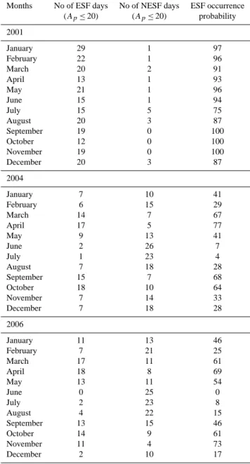
The top panel of Fig. 3 shows the monthly variation in the percentage occurrence of ESF for the three years. Clearly a very high percentage occurrence (above ∼85%) is ob-served in all the months during 2001, except in July where the value is slightly less (∼75%). During 2004, the highest percentage occurrence (above∼65%) is observed during the equinoctial months (March–April and September–October) and lowest (∼4%) during the summer solstitial months of June–July. The percentage occurrence probability during the other months is between 30–50%. During 2006, the high-est percentage occurrence (above∼60%) is observed during the equinoctial months of March–April and October and also during the winter month of November. The lowest value of
∼8% is observed in the month of July. In June, however, the percentage occurrence probability is zero. In all the other months, the occurrence probability is between 30–50%.
The bottom panel of Fig. 3 shows the 10 day mean varia-tions of the parameter “E” on ESF days of each month. The middle panel of Fig. 3 shows an identical representation for Vz. A comparison between the percentage occurrence of ESF and the mean variations of the parameter “E” andVzindicate a reasonably good correspondence between them.
3.4 Possible cause for the linkage of the parameter “E” withVz
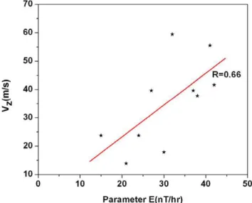
To investigate the possible cause and effect relationship be-tween the parameter “E” andVz, we chose one international quiet day (on which ESF was observed) of each month for the year 2001 and calculated the parameter “E” on each of these days. Figure 4a shows the scatter plot of the parameter “E” versusVzfor these days. Quite evidently, a fairly good pos-itive correlation (R=0.66) is observed between the two pa-rameters. The possible relationship between parameter “E” andVzcan be thought of as follows: a large value for the pa-rameter “E” means that the EIA is evolving at a faster rate or rather the strength of the EIA is getting enhanced. The inten-sification of EIA reduces the plasma density over the mag-netic equator (trough of EIA) and simultaneously increases the plasma density over the crest regions. The decrease in the plasma density over the magnetic equator reduces the ion drag on the neutrals and hence the zonal wind is enhanced prior to sunset. The enhanced anomaly will also increase the F- to E-region flux tube integrated Pedersen conductiv-ity (Crain et al., 1993). Both these changes in turn produce a large eastward electric field and hence causes a large post sunset vertical drift of the F-layer i.e. a larger value of the parameter “E” in turn is related with a larger value ofVz.
4234 V. Sreeja et al.: Observational evidence for the plausible linkage of EEJ
Table 1. Variations in the monthly occurrence pattern of the ESF and the non-ESF days along with the ESF percentage occurrence probability during each month of the solar maximum year of 2001, moderate activity year of 2004 and the solar minimum year of 2006.
Months No of ESF days No of NESF days ESF occurrence (Ap≤20) (Ap≤20) probability 2001
January 29 1 97
February 22 1 96
March 20 2 91
April 13 1 93
May 21 1 96
June 15 1 94
July 15 5 75
August 20 3 87
September 19 0 100
October 12 0 100
November 19 0 100
December 20 3 87
2004
January 7 10 41
February 6 15 29
March 14 7 67
April 17 5 77
May 9 13 41
June 2 26 7
July 1 23 4
August 7 18 28
September 15 7 68
October 18 10 64
November 7 14 33
December 7 18 28
2006
January 11 13 46
February 7 21 25
March 17 11 61
April 18 8 69
May 13 11 54
June 0 25 0
July 2 23 8
August 4 22 15
September 13 15 46
October 14 9 61
November 11 4 73
December 2 10 17
the years of 2001, 2004 and 2006 irrespective of the seasons. Discrete intervals of 5 nT/h for the parameter “E” have been used to study the response ofVzto this parameter. It is clear from this figure that on an average, Vzexhibits a positive re-lationship with the parameter “E” during the solar maximum year of 2001 and the moderate activity year of 2004. But, for the solar minimum year of 2006, it is very difficult to de-duce such a relation, as the number of ESF events itself was very low. The large error bars in the plot indicate that for a given parameter “E”, there is a large scatter in the value of
Vz. This feature suggests thatVzdoes not uniquely depend on the magnitude of parameter “E”, though the trends appear to come out well.
3.5 Monthly variations in the Maximum E×B drift (Vz) corresponding to the observed variations of the parameter “E”
Figure 5 is a gross statistical picture showing the monthly variability in the parameter “E” and maximumVzalong with the time of maximumVzand the onset time of ESF for the period under study. As is clear from the figure, maximum Vz values above 15 m/s are characteristic of all the months of 2001, with peak values of Vz more than 35 m/s in the equinoctial and the winter solstitial months, where the ESF occurrence probability is also more than 90%. The time of occurrence of maximum Vz is observed to be centered around 19:00 IST or earlier during almost all the months of 2001. The fairly larger occurrence probability of ESF even during the winter solstitial months can also be explained on the basis of the largerVz values and the earlier occurrence time of Vz during these months. Another interesting rela-tionship (shown in the top panel of the Fig. 5) observed dur-ing 2001 is between the average onset time of ESF andVz, which indicate that the earlier onset time of ESF during the equinoctial months are associated with the larger values of Vz. This feature is also manifested, though less clearly, dur-ing the moderate activity year of 2004 and the solar mini-mum year of 2006, in association with the ESF events of the equinoctial months. The onset time of ESF during the differ-ent months of 2004 is between 19:00 and 20:00 IST, whereas during 2006, the onset time is delayed upto about 20:00 IST. A comparatively lower value ofVzand later occurrence time (beyond 19:00 IST) is also reflected in the ESF occurrence during 2004 and 2006. Of course these observed results con-form to the already known fact that both the time ofVz and the onset of ESF are basically controlled by the sunset time (Maruyama and Matuura, 1984).
These observations show that a large upwardVzvalue and its early occurrence time in the post sunset hours are the most favourable conditions for the onset of ESF over Trivandrum. This is in contrast to the observation of a largeVz and its late occurrence time in the post sunset hours as reported by Maruyama (1988) and Fejer et al. (1999) in the case of ESF occurrence over Jicamarca during the summer months. Over the Indian region, Vyas and Chandra (1991) reported that a delayed afternoon zonal F-region drift reversal was associ-ated with ESF occurrence.
V. Sreeja et al.: Observational evidence for the plausible linkage of EEJ 4235
≤
616
Fig. 3. The percentage of days of ESF occurrence on all the magnetically quiet days (Ap≤20) of each month of 2001, 2004 and 2006 (top panel). The middle panel shows the 10 day mean variations in theVzvalues on ESF days of the month. The bottom panel shows an identical representation for the “parameter E”.
growth rate of the R-T instability causing ESF. In contrast, the comparatively lower values of Vz observed during the summer solstitial months of May, June, July and August could not lead to the uplifting of the F-layer to the higher al-titudes. Thus, the percentage occurrence of ESF is also com-paratively lower during these months, but still much larger than that observed during the equinoctial months of the so-lar minimum year, where theVz values are comparatively lower. The observed inter-dependence between the different parameters thus seem to be useful in arriving at a gross rep-resentative estimate of the parameter “E”, which would be a fairly good statistical estimate of the PRE that assists the R-T instability growth, which is very much in accordance with earlier results (Sultan, 1996; Fejer et al., 1999; Kudeki et al., 1999; Whalen, 2002).
4 Summary and conclusions
The details of the observational results relating to the plausi-ble linkage of the daytime EEJ related electric field variabil-ities with the occurrence of ESF under magnetically quiet conditions during different seasons of the solar maximum,
627
628
629
630
631
632
633
634
635
636
Fig. 4a. Scatter plot of the parameter “E” versusVzfor some inter-national quiet days of each month during the year 2001.
4236 V. Sreeja et al.: Observational evidence for the plausible linkage of EEJ
650
Fig. 4b. Plot of the averageVz, with the standard deviation, against the “parameter E”, taken in intervals of 5 nT/h, for the solar maximum, moderate and minimum years of 2001, 2004 and 2006.
667
Fig. 5. Monthly mean variations of the “parameter E”, maximum F-region vertical drift velocity (Vz), its occurrence time and the onset time of ESF with the corresponding standard deviation for 2001, 2004 and 2006.
1. The detailed investigation has brought out some inter-esting results on the similarities in the monthly and sea-sonal variabilities of the various E- and F-region related
V. Sreeja et al.: Observational evidence for the plausible linkage of EEJ 4237 2. These features are manifested with a very good
similar-ity in the mean monthly and seasonal variabilities in the EEJ electric field related parameter “E” and theE×B
drift velocity (Vz)in the post sunset hours. These fea-tures can be useful for making a statistical inference of the post sunset F-region behavior from the daytime EEJ electric field characteristics which are directly obtained from the ground magnetic field variations. The results also enable us to make a quantitative estimation of the meanVzas a function of the magnitude of the parameter “E” on a monthly and seasonal basis.
The present study shows that the occurrence of ESF over dif-ferent seasons is evidently correlated with the variations in the magnitude of the parameter “E” andVz. The observed statistical correlation of these parameters with ESF events in the equinoctial and winter months of the solar minimum year and in all the months of the solar maximum and mod-erate year show that the ionosphere is lifted to higher alti-tudes where the gravitational drift term is dominant in the R-T instability growth rate, leading to the development of ESF, when the upward drift velocities are larger. Apart from the magnitude ofVz, the time of occurrence of the maximum value ofVz is also observed to play a dominant role in the occurrence of ESF. LargerVzand its earlier occurrence time are observed to provide the favorable conditions for the ear-lier onset time of ESF. The earear-lier onset time of ESF during the equinoctial months and later onset time during the sol-stitial months thus follow from the seasonal patterns of the parameter “E” andVzvariations.
It should be emphasized that the results of the present study are based on an analysis of three years of data-one year of solar maximum, one year of moderate activity and one year of solar minimum. It is to be expected that the relation-ship between parameter “E” andVzduring the magnetically quiet days of other years should not deviate much from the presently arrived relationships. Hence the information on the parameter “E”, as derived from the magnetometer measure-ments, seems to provide a simple method of establishing di-rect relationships the between parameter “E” andVzthrough the nature of their gross variabilities.
It should also be mentioned that a comprehensive under-standing of the ESF phenomenon under varying seasonal and solar activity conditions is extremely important with our in-creased dependence on satellite based communications and geodesy. As already mentioned, ESF is an outcome of the R-T instability in the equatorial ionosphere which in turn is controlled by both ionospheric and neutral atmospheric pa-rameters like plasma density scale length (L), ion-neutral collision frequency(νin)and neutral winds in addition to the main driving factor viz: the gravity(g). The generalized ex-pression for the local growth rate of the R-T instability is given by the equation (Sekar and Raghavarao, 1987; Kelley, 1989),
γ= 1
L
g
νin
+EX
B +Wx ν
in i
−Wz
(1) whereWx andWz are the zonal and vertical winds respec-tively,EXis the zonal electric field in the F-region,Bis the geomagnetic field andi is the ion gyro- frequency.
As it is clear from the Eq. (1), the growth rate depends mainly onLandνin. At lower heights, the growth rate of the instability would decrease due to increasedνin andL. This along with the reduced zonal electric field during the solar minimum period would result in a low occurrence rate of ESF. During the solar maximum period, the comparatively larger value of the electric field would lift the F-layer to high enough altitudes (lowerνinandL), where the conditions are more favourable for the triggering of the R-T instability. The larger percentage occurrence of ESF during solar maximum period directly follows from these favourable conditions.
Acknowledgements. This work was supported by Department of
Space, Government of India. One of the authors, V. Sreeja, grate-fully acknowledges the financial assistance provided by the Indian Space Research Organization through Research Fellowship. The authors thank the Indian Institute of Geomagnetism (IIG), Mumbai, India for providing the magnetic field values.
Topical Editor M. Pinnock thanks H. Chandra and another anonymous referee for their help in evaluating this paper.
References
Aarons, J.: The longitudinal morphology of Equatorial F-layer ir-regularities relevant to their occurrence, Space Sci. Rev., 63, 209–243, 1993.
Abdu, M. A., Ramkumar, T. K., Batista, I. S., Brum, C. G. M., Takahasi, H., Reinisch, B. W., and Sobral, J. H. A.: Planetary wave signatures in the equatorial atmosphere-ionosphere system, and mesosphere- E- and F-region coupling, J. Atmos. Terr. Phys., 68, 509–522, 2006.
Abdu, M. A., Sobral, J. H. A., and Batista, I. S.: Equatorial spread-F statistics: some problems relevant to ESspread-F description in the IRI scheme, Adv. Space Res., 25(1), 113–124, 2000.
Alex, S., Koparker, P. V., and Rastogi, R. G.: Spread F and ioniza-tion anomaly belt, J. Atmos. Terr. Phys., 51, 371–379, 1989. Anderson, D., Anghel, A., Yumoto, K., Ishitsuka, M., and Kudeki,
E.: Estimating daytime vertical ExB drift velocities in the equa-torial F-region using ground-based magnetometer observations, Geophys. Res. Lett., 29, 1596, doi:10.1029/2001GL014562, 2002.
Basu, S., Kudeki, E., Basu, Su., Weber, E. J., Valladares, C. E., Sheehan, R., Meriwether, J. W., Kuenzler, H., Bishop, G. J., and Biondi, M. A.: Scintillations, Plasma drifts, and neutral winds in the equatorial ionosphere after sunset, J. Geophys. Res., 101, 26795–26809, 1996.
Batista, I. S., Abdu, M. A., and Bittencourt, J. A.: Equatorial F region vertical plasma drifts: seasonal and longitudinal asymme-tries in the American sector, J. Geophys. Res., 91, 12055–12064, 1986.
4238 V. Sreeja et al.: Observational evidence for the plausible linkage of EEJ
Chandra, H. and Rastogi, R. G.: Solar cycle and seasonal variation of spread F near the magnetic equator, J. Atmos. Terr. Phys., 32, 439–443, 1970.
Crain, D. J., Heelis, R. A., and Bailey, G. J.: Effects of electrical coupling on equatorial ionosphere plasma motions: When is the F region a dominant driver in the low-latitude dynamics?, J. Geo-phys. Res., 98, 6033–6037, 1993.
Devasia, C. V., Jyoti, N., Vishwanathan, K. S., Subbarao, K. S., Tiwari, D., and Sridhran, R.: On the plausible linkage of ther-mospheric meridional winds with equatorial spread F, J. Atmos. Solar Terr. Phys., 64, 1–12, 2002.
Devasia, C. V., Sreeja, V., and Ravindran, S.: Solar cycle dependent characteristics of the equatorial blanketingEslayers and associ-ated irregularities, Ann. Geophys., 24, 2931–2947, 2006, http://www.ann-geophys.net/24/2931/2006/.
Dunford, E.: The relationship between the ionospheric equatorial anomaly and the E-region current system, J. Atmos. Solar Terr. Phys., 29, 1489–1498, 1967.
Eccles, J. V.: A modeling investigation of the evening pre-reversal enhancement of the zonal electric field in the equatorial iono-sphere, J. Geophys. Res., 103, 26709–26719, 1998.
Farley, D. T., Bonelli, E., Fejer, B. G., and Larsen, M. F.: The pre-reversal enhancement of the zonal electric field in the equatorial ionosphere, J. Geophys. Res., 91, 13723–13728, 1986.
Fejer, B. G., Scherliess, L., and de Paula, E. R.: Effects of the verti-cal plasma drift velocity on the generation and evolution of equa-torial spread F, J. Geophys. Res., 104, 19854–19869, 1999. Fejer, B. G.: Low latitude electrodynamic plasma drifts: A review,
J. Atmos. Terr. Phys., 53, 677–693, 1991.
Fejer, B. G. and Kelley, M. C.: Ionospheric irregularities, Rev. Geo-phys., 18, 401–454, 1980.
Haerendel, G. and Eccles, J. V.: The role of the equatorial electro-jet in the evening ionosphere, J. Geophys. Res., 97, 1181–1197, 1992.
Hysell, D. L. and Burcham, J.: Long term studies of equatorial spread F using the JULIA radar at Jicamarca, J. Atmos. Solar Terr. Phys., 64, 1531–1543, 2002.
Hysell, D. L.: An overview and synthesis of plasma irregularities in equatorial spread F, J. Atmos. Solar Terr. Phys., 62, 1037–1056, 2000.
Jayachandran, P. T., Sri Ram, P., Somayajulu, V. V., and Rama Rao, P. V. S.: Effect of equatorial ionization anomaly on the occur-rence of spread-F, Ann. Geophys., 15, 255–262, 1997,
http://www.ann-geophys.net/15/255/1997/.
Kelley, M. C.: The Earth’s Ionosphere, Academic Press, San Diego, 75–125, 1989.
Kelley, M. C., Ilma, R. R., and Crowley, G.: On the origin of pre-reversal enhancement of the zonal equatorial electric field, Ann. Geophys., 27, 2053–2056, 2009,
http://www.ann-geophys.net/27/2053/2009/.
Krishna Murthy, B., Hari, S. S., and Somayajulu, V. V.: Nighttime equatorial thermospheric meridional winds from ionospheric h’F data, J. Geophys. Res., 95(A4), 4307–4310, 1990.
Kudeki, E., Bhattacharyya, S., and Woodman, R. F.: A new ap-proach in incoherent scatter F region ExB drift measurements at Jicamarca, J. Geophys. Res., 104, 28145–28162, 1999.
Liu, L., Luan, X., Wan, W., Lei, J., and Ning, B.: Solar activity vari-ations of equivalent winds derived from global ionosonde data, J. Geophys. Res., 109, A12305, doi:10.1029/2004JA010574, 2004.
Maruyama, T.: A diagnostic model for equatorial spread F 1. Model description and application to electric fields and neutral wind ef-fects, J. Geophys. Res., 93, 14611–14622, 1988.
Maruyama, T. and Mattura, N.: Longitudinal variability of annual changes in activity of equatorial spread F and plasma bubbles, J. Geophys. Res., 89, 10903–10912, 1984.
Maynard, N. C., Aggson, T. L., Herrero, F. A., Liebrecht, M. C., and Sabu, J. L.: Average equatorial zonal and vertical ion drifts determined from San Marco D electric field measurements, J. Geophys. Res., 100, 17465–17479, 1995.
Mendillo, M., Meriwether, J., and Biondi, M.: Testing the thermo-spheric neutral wind suppression mechanism for day-to-day vari-ability of equatorial spread F, J. Geophys. Res., 106, 3655–3663, 2001.
Raghavarao, R., Nageswararao, M., Sastri, J. H., Vyas, G. D., and Sriramarao, M.: Role of equatorial ionization anomaly in the ini-tiation of equatorial spread F, J. Geophys. Res., 93, 5959–5964, 1988.
Raghavarao, R., Sharma, P., and Sivaraman, M. R.: Correlation of ionization anomaly with the intensity of the electrojet, Space Res., 18, 277–280, 1978.
Rastogi, R. G. and Rajaram, G.: Electrojet effects on the equatorial F region during magnetically quiet and disturbed days, Ind. J. Pure Appl. Phys., 9, 531–536, 1971.
Rishbeth, H.: The F-region dynamo, J. Atmos. Terr. Phys., 43, 387– 392, 1981.
Rush, C. M. and Richmond, A. D.: The relationship between the structure of the equatorial anomaly and the strength of the equa-torial electrojet, J. Atmos. Terr. Phys., 35, 1171–1180, 1973. Sastri, J. H.: Longitudinal dependence of equatorial F region
verti-cal plasma drifts in the dusk sector, J. Geophys. Res., 101, 2445– 2452, 1995.
Sastri, J. H.: Equatorial anomaly in F-region-A review, Indian J. Radio Space Phys., 19, 225–240, 1990.
Scherliess, L. and Fejer, B. G.: Radar and satellite global equatorial F region vertical drift model, J. Geophys. Res., 104, 6829–6842, 1999.
Sekar, R. and Raghavarao, R.: Role of vertical winds on the Rayleigh-Taylor instabilities of the night time equatorial iono-sphere, J. Atmos. Terr. Phys., 49, 981–985, 1987.
Sridharan, R., Raju, D. P., Raghavarao, R. and Ramarao, P. V. S.: Precursor to equatorial spread-F in OI 630.0 nm dayglow, Geo-phys. Res. Lett., 21, 2797–2800, 1994.
Sultan, P.: Linear theory and modeling of the Rayleigh-Taylor in-stability leading to the occurrence of equatorial spread F, J. Geo-phys. Res., 101, 26875–26891, 1996.
Thampi, S. V., Sudha Ravindran, Tarun Kumar Pant, Devasia, C. V., Sreelatha, P., and Sridharan, R.: Deterministic prediction of post-sunset ESF based on the strength and asymmetry of EIA from ground based TEC measurements: Preliminary results, Geophys. Res. Lett., 33, L13103, doi:10.1029/2006GL026376, 2006. Vyas, G. D. and Chandra, H.: Ionospheric zonal drift reversal and
equatorial spread F, Ann. Geophys., 9, 299–303, 1991.
Whalen, J. A.: Dependence of equatorial bubbles and bottomside Spread F on season, magnetic activity, and EXB drift veloc-ity during solar maximum, J. Geophys. Res., 107(A2), 1024, doi:10.1029/2001JA000039, 2002.