mizuRoute version 1: a river network routing tool for a continental domain water resources applications

(1)

GMDD

8, 9415–9449, 2015

mizuRoute version 1

N. Mizukami et al.

Title Page

Abstract Introduction

Conclusions References

Tables Figures

◭ ◮

Back Close

Full Screen / Esc

Printer-friendly Version Interactive Discussion

Discussion

P

a

per

|

Discussion

P

a

per

|

Discussion

P

a

per

|

Discussion

P

a

per

|

Geosci. Model Dev. Discuss., 8, 9415–9449, 2015 www.geosci-model-dev-discuss.net/8/9415/2015/ doi:10.5194/gmdd-8-9415-2015

This discussion paper is/has been under review for the journal Geoscientific Model Development (GMD). Please refer to the corresponding final paper in GMD if available.

mizuRoute version 1: a river network

routing tool for a continental domain

water resources applications

N. Mizukami1, M. P. Clark1, K. Sampson1, B. Nijssen2, Y. Mao2, H. McMillan3, R. J. Viger4, S. L. Markstrom4, L. E. Hay4, R. Woods5, J. R. Arnold6, and

L. D. Brekke7

1

National Center for Atmospheric Research, Boulder, CO, USA

2

University of Washington, Seattle, WA, USA

3

National Institute of Water and Atmospheric Research, Christchurch, New Zealand

4

United States Geological Survey, Denver, CO, USA

5

University of Bristol, Bristol, UK

6

US Army of Corps of Engineers, Seattle, WA, USA

7

Bureau of Reclamation, Denver, CO, USA

Received: 8 September 2015 – Accepted: 15 October 2015 – Published: 2 November 2015 Correspondence to: N. Mizukami (mizukami@ucar.edu)

(2)

GMDD

8, 9415–9449, 2015

N. Mizukami et al.

Title Page

Tables Figures

◭ ◮

Back Close

Full Screen / Esc

Discussion

P

a

per

|

Discussion

P

a

per

|

Discussion

P

a

per

|

Discussion

P

a

per

|

Abstract

This paper describes the first version of a stand-alone runoffrouting tool, mizuRoute, which post-processes runoffoutputs from any distributed hydrologic model or land sur-face model to produce spatially distributed streamflow at various spatial scales from headwater basins to continental-wide river systems. The tool can utilize both

tradi-5

tional grid-based river network and vector-based river network data, which includes river segment lines and the associated drainage basin polygons. Streamflow estimates at any desired location in the river network can be easily extracted from the output of mizuRoute. The routing process is simulated as two separate steps. The first is hillslope routing, which uses a gamma distribution to construct a unit-hydrograph that represents

10

the transport of runofffrom a hillslope to a catchment outlet. The second step is river channel routing, which is performed with one of two routing scheme options: (1) a kine-matic wave tracking (KWT) routing procedure; and (2) an impulse response function– unit hydrograph (IRF-UH) routing procedure. The mizuRoute system also includes tools to pre-process spatial river network data. This paper demonstrates mizuRoute’s

capa-15

bilities with spatially distributed streamflow simulations based on river networks from the United States Geological Survey (USGS) Geospatial Fabric (GF) dataset, which contains over 54 000 river segments across the contiguous United States (CONUS). A brief analysis of model parameter sensitivity is also provided. The mizuRoute tool can assist model-based water resources assessments including studies of the impacts

20

of climate change on streamflow.

1 Introduction

The routing tool described in this paper post-processes runoff outputs from macro-scale hydrologic models or land surface models (hereafter we use “hydrologic model” to refer to both types of model) to estimate spatially distributed streamflow along the

25

(3)

GMDD

8, 9415–9449, 2015

N. Mizukami et al.

Title Page

Tables Figures

◭ ◮

Back Close

Full Screen / Esc

Discussion

P

a

per

|

Discussion

P

a

per

|

Discussion

P

a

per

|

Discussion

P

a

per

|

Japanese). The motivation for mizuRoute’s development was to enable continental do-main evaluations of hydrologic simulations for water resources assessments, such as studies of the impacts of climate change on streamflow. The mizuRoute tool is suitable for processing of ensembles of multi-decadal runoffoutputs because the tool is stan-dalone and easily applied in a parallel mode. The mizuRoute tool is also designed to

5

output streamflow estimates at all river segments in the river network across the do-main of interest at each time step, facilitating the further spatial and temporal analysis of the estimated streamflow.

The paper proceeds as follows. Section 2 reviews existing river routing models. Sec-tion 3 describes the hillslope and river routing schemes used in mizuRoute. SecSec-tion 4

10

provides an overview of the workflow of mizuRoute from preprocessing hydrologic model output to simulating streamflow in the river network. Section 5 demonstrates streamflow simulations in river systems over the contiguous United States. Finally, a summary and future work are discussed in Sect. 6.

2 Existing river routing models

15

The water resources and Earth System Modeling communities have developed a wide spectrum of river routing schemes of varying complexity (Clark et al., 2015). For ex-ample, the US Army Corps of Engineers (USACE) has developed a stand-alone river modeling system called Hydrologic Engineering Center-River Analysis System (HEC-RAS; Brunner, 2001). HEC-RAS offers various hydraulic routing schemes, ranging

20

from simple uniform flow to one-dimensional (1-D) Saint-Venant equations for unsteady flow. HEC-RAS has been popular among civil engineers for river channel design and floodplain analysis where surveyed river geometry and physical channel properties are available. At the continental to global scale, unit-hydrograph approaches have been used (e.g., Nijssen et al., 1997; Lohmann et al., 1998; Goteti et al., 2008;

Za-25

(4)

GMDD

8, 9415–9449, 2015

N. Mizukami et al.

Title Page

Tables Figures

◭ ◮

Back Close

Full Screen / Esc

Discussion

P

a

per

|

Discussion

P

a

per

|

Discussion

P

a

per

|

Discussion

P

a

per

|

Clark et al., 2015), simplified Saint-Venant equations such as the kinematic wave or diffusive wave equation (e.g., Arora and Boer, 1999; Lucas-Picher et al., 2003; Ko-ren et al., 2004; Yamazaki et al., 2011, 2013; Li et al., 2013; Gochis, 2015; Yucel et al., 2015) or non-dynamical hydrologic routing methods such as Muskingum rout-ing (e.g., David et al., 2011). Despite their computational cost, dynamic or diffusive

5

wave models are attractive for relatively flat floodplain regions such as along the Ama-zon River where backwater effects on the flood wave are significant (Paiva et al., 2011; Yamazaki et al., 2011; Miguez-Macho and Fan, 2012). At the other end of the spec-trum, simpler, non-dynamic routing schemes, such as the unit hydrograph approach, estimate the flood wave delay and attenuation, but no other streamflow variables such

10

as flow velocity and flow depth.

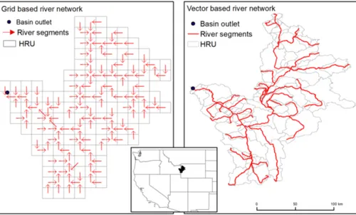
One of the key issues for large scale river routing, besides the choice of the routing scheme, is the degree of abstraction in the representation of the river network (Fig. 1). A vector-based representation of the river network refers to a collection of hydrologic response units (HRUs) that are delineated based on topography or catchment

bound-15

ary. River segments in the vector-based river network, represented by lines, meander through HRUs and connect upstream with downstream HRUs. On the other hand, in the grid-based river network, the HRU is represented by a grid box and river segments con-nect neighboring grid boxes based on the flow directions. Vector-based river networks are better than coarser resolution (e.g.>1 km) gridded river networks at preserving

20

fine-scale features of the river system such as tortuosity, therefore representing more accurate sub-catchment areas and river segment lengths.

For large scale applications, many studies have developed and evaluated methods to upscale fine resolution flow direction grids (∼1 km or less) to a coarser resolution

(_∼10 km or more) to match hydrologic model resolution and/or reduce the cost of

rout-25

(5)

rep-GMDD

8, 9415–9449, 2015

N. Mizukami et al.

Title Page

Tables Figures

◭ ◮

Back Close

Full Screen / Esc

Discussion

P

a

per

|

Discussion

P

a

per

|

Discussion

P

a

per

|

Discussion

P

a

per

|

resentation of the drainage area. Newer upscaling methods are designed to also pre-serve fine-scale flow path length (e.g., Yamazaki et al., 2009; Wu et al., 2011). More recent river routing models have also begun to employ vector-based river networks (Goteti et al., 2008; David et al., 2011; Paiva et al., 2011, 2013; Lehner and Grill, 2013; Yamazaki et al., 2013).

5

3 Runoffrouting in mizuRoute

The runoff routing in mizuRoute provides more flexibility in continental domain rout-ing applications. The mizuRoute framework enables model flexibility in two ways: first, mizuRoute can be used to simulate streamflow for both grid- and vector-based river networks. Given either type of river network data, mizuRoute offers an option to route

10

flow along all the river segments in the river network data or route runoffat an outlet segment specified by a user. With the latter option, routing computation is performed only in the upstream river network of the specified outlet, which reduces the compu-tational cost. Second, the modular structure of the mizuRoute framework offers the flexibility to configure multiple routing schemes. The current version of mizuRoute

in-15

cludes two different type of river routing schemes: (1) kinematic wave tracking (KWT) routing and (2) impulse response function–unit hydrograph (IRF-UH) routing, mimick-ing the Lohmann et al. (1996) model. This flexibility offers new capabilities not present in existing routing models. One capability is to provide an opportunity to explore routing model uncertainties originating from the representation of the river system and routing

20

scheme differences (equations and parameters) separately.

The mizuRoute tool uses a two-step process to route basin runoff. First, basin runoff is routed from each hillslope to the river channel using a gamma-distribution-based unit-hydrograph. This allows the representation of ephemeral channels or channels too small to be included in the river network. Second, using one of the two channel routing

25

(6)

GMDD

8, 9415–9449, 2015

N. Mizukami et al.

Title Page

Tables Figures

◭ ◮

Back Close

Full Screen / Esc

Discussion

P

a

per

|

Discussion

P

a

per

|

Discussion

P

a

per

|

Discussion

P

a

per

|

hydrologic model, typically an hourly or daily time step. The following sub-sections provide descriptions of the two routing steps.

3.1 Hillslope routing

Hillslope routing accounts for the time of concentration (Tc) of a local catchment (i.e., an HRU) to estimate temporally delayed runoff(or discharge) at the outlet of the HRU

5

from runoffcomputed by a hydrologic model.

For hillslope routing mizuRoute uses a simple two-parameter Gamma distribution as a unit-hydrograph to route instantaneous runofffrom a hydrologic model to a HRU outlet. The Gamma distribution is expressed as:

γ(t:a,θ)= 1 Γ(a)θat

a₋1_e−tθ ₍₁₎

10

wheretis time [T],ais a shape parameter [₋] (a >0), andθis a time-scale parameter [T]. Both the shape and time scale parameters determine the peak time (mean of the distribution:aθ) and flashiness (variance of the distribution:aθ2) of the unit-hydrograph and depend on the physical catchment characteristics. Convolution of the gamma dis-tribution with the runo_ff depth series is used to compute the fraction of runo_ff at the

15

current time which is discharged to its corresponding river segment at each future time as follows:

q(t)=

tmax

Z

0

γ(s:a,θ)_·R(t₋s) ds (2)

whereqis delayed runoffor discharge [L3T−1_{] at time step}_t _[T],_R _{is HRU total runo}_ff depth [L3T−1_{] from hydrologic model, and tmax is the maximum time length for the}

20

(7)

GMDD

8, 9415–9449, 2015

N. Mizukami et al.

Title Page

Tables Figures

◭ ◮

Back Close

Full Screen / Esc

Discussion

P

a

per

|

Discussion

P

a

per

|

Discussion

P

a

per

|

Discussion

P

a

per

|

3.2 River channel routing

Two different river channel routing schemes are implemented in mizuRoute: (1) the kinematic wave tracking (KWT) routing procedure; and (2) the impulse response function–unit hydrograph (IRF-UH) routing procedure. Both schemes are based on the 1-D Saint-Venant equations that describe flood wave propagation through a river

chan-5

nel. The one-dimensional conservation equations for continuity (Eq. 3) and momentum (Eq. 4) are

∂q ∂x+

∂A

∂t =0 (3)

∂v ∂t +v

∂v ∂x+g

∂y

∂x−g(S0−Sf)=0 (4)

whereq is discharge [L3T−1] at time step t [T] and location x [L] in a river network,

10

A is cross-sectional flow area [L2], v is velocity [L T−1_], _y _{is depth of flow [L],} _S

0 is

channel slope [₋], Sf is friction slope [−], and g is gravitational constant [L T− 2

]. The continuity equation (Eq. 3) assumes that no lateral flow is added to a channel segment. The following sub-sections describe the two routing schemes.

3.2.1 Kinematic wave tracking (KWT)

15

In contrast with several other kinematic routing models that solve a kinematic wave equation with the numerical schemes (e.g., Arora and Boer, 1999; Lucas-Picher et al., 2003; Koren et al., 2004), the KWT method computes a wave speed or a celerity for the runoff(or discharge) that enters an individual stream segment from the corre-sponding HRU at each time step using kinematic approximation (Goring, 1994; Clark

20

(8)

GMDD

8, 9415–9449, 2015

N. Mizukami et al.

Title Page

Tables Figures

◭ ◮

Back Close

Full Screen / Esc

Discussion

P

a

per

|

Discussion

P

a

per

|

Discussion

P

a

per

|

Discussion

P

a

per

|

In the kinematic wave approximation with the assumption that the channel is rectan-gular and hydraulically wide (channel width_≫y), the wave celerityC[L T−1_{] is a} func-tion of channel widthw [L], Manning’s coefficientn[−], channel slope S0[−] and

dis-chargeq[L3T−1_{]. Further details are provided in Appendix A. Among the four variables,} the channel slopeS0 is provided in the river network data and discharge is computed 5

with hillslope routing for the headwater basin, or/and updated via routing from the up-stream segment. The other two variables, Manning’s coefficient n and river width w, are much more difficult to measure or estimate. The river width is determined with the following width-drainage area relationship (Booker, 2010):

w=Wa·Abups (5)

10

whereW_a is a width factor [₋], Aups is the total upstream basin area [L 2

] and b is an empirical exponent equal to 0.5. The width factor W_a and the Manning’s coefficient n

are treated as model parameters as shown in Table 1.

The KWT routing starts with ordering all the segments in the processing sequence from upstream to the downstream segments. The KWT routing is performed at each

15

segment in the processing order at each time step. The procedures of the KWT routing method are detailed as follows:

1. The first routine obtains the information on the waves that reside in the segment at a given time step: the waves routed from the upstream segments, the wave that remains in this current segment form the previous time step, and the wave

20

generated from the runoff from local HRUs during the current time step. Three state variables of the waves are kept in the memory: discharge, time at which the wave enters the segment, and time at which the wave is expected to exit the segment (assign the missing value to the waves routed from the upstream segment, and computed in step 3). At the first time step, only wave from local

25

(9)

GMDD

8, 9415–9449, 2015

N. Mizukami et al.

Title Page

Tables Figures

◭ ◮

Back Close

Full Screen / Esc

Discussion

P

a

per

|

Discussion

P

a

per

|

Discussion

P

a

per

|

Discussion

P

a

per

|

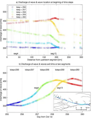
2. The second routine (wave removal routine) reduces the memory usage as well as the processing time for the wave routing (the next step). The number of the waves in the segment is limited to a predefined number (20 by default). In Fig. 2, the threshold of the number of wave in the segment is set to 100. To determine which waves can be removed, first, difference between the discharge of the wave

5

and linearly interpolated discharge values between its two neighboring waves is computed for all the waves, and then the wave that produces the least difference (from the interpolated discharge) is removed so that loss of wave mass is mini-mized. This process is repeated until the number of waves become lower than the threshold.

10

3. The third routine performs the wave routing over a given river segment. In the rout-ing routine, the celerity of each wave in the segment is computed with Eq. (A6), and then the time at which each wave is expected to exit the river segment is updated. If the exit time occurs before the end of the time step, the wave is prop-agated to the downstream segment and flagged as “exited”. The exit time then

15

becomes the time the wave entered the downstream segment. Otherwise, the wave is flagged as “not-exited”, and remains in the current segment. Figure 2b shows the discharge of the waves against the exit times of the corresponding waves at segments 4 and 13. As a reference, the end of each time step is shown as a vertical line. In Fig. 2b, the waves situated before the end of time step exits

20

the segments at a given time step. The routing routine checks for (and corrects) the special case of a kinematic shock. A kinematic shock is a sudden rise in the flow depth, thus an increase in the discharge at a fixed location, and occurs when a faster-moving wave successively overtakes multiple slower-waves to build a steep wave front. It occurs in models due to the kinematic approximation; in

re-25

(10)

GMDD

8, 9415–9449, 2015

N. Mizukami et al.

Title Page

Tables Figures

◭ ◮

Back Close

Full Screen / Esc

Discussion

P

a

per

|

Discussion

P

a

per

|

Discussion

P

a

per

|

Discussion

P

a

per

|

one, and the celerity of the merged wave is updated with the following equation;

Cmerge=∆ q

∆A=

∆q

w∆y (6)

whereCmerge is the merged wave celerity [L T− 1

], ∆q and ∆Aare differences in discharge [L3T−1

] and cross-sectional flow area [L2T−1

], respectively, between slower and faster waves. Note that Eq. (3) is the mathematical definition of the

5

wave celerity. Since we assume the rectangular channel whose width is constant for each segment, the merged celerity Cmerge is a function of the flow depth y,

which is computed with Eq. (A3).

4. Finally, the time step averaged discharge (streamflow) is computed by temporal integration of discharge of all the waves that exit the segment during the time step.

10

Temporal integral of wave discharge is visualized in Fig. 2b as the area enclosed by the discharge curve formed by all the exiting waves between the beginning and end of time step.

3.2.2 Impulse response function-unit hydrograph (IRF-UH)

The IRF-UH method mimics the river routing model of Lohmann et al. (1996), which

15

has been used to route flows from gridded land surface models such as the Variable Infiltration Capacity model (VIC; Liang et al., 1996). The only di_fference between the current tool and the Lohmann routing tool is the way in which the river network is defined. The Lohmann routing model is designed as a grid-based model as shown in Fig. 1 to ease the coupling with grid-based land surface models. In mizuRoute, the

20

(11)

GMDD

8, 9415–9449, 2015

N. Mizukami et al.

Title Page

Tables Figures

◭ ◮

Back Close

Full Screen / Esc

Discussion

P

a

per

|

Discussion

P

a

per

|

Discussion

P

a

per

|

Discussion

P

a

per

|

The mathematical developments of IRF-UH are based on one-dimensional diffusive wave equation derived from the 1-D Saint-Venant equations (Eqs. 4 and 5):

∂q ∂t =D

∂2q ∂x2−C

∂q

∂x (7)

where parametersCandDare wave celerity [L T−1] and diffusivity [L2T−1], respectively. The complete derivation from Eqs. (4) and (5) to Eq. (7) is given in Appendix B.

5

Equation (4) can be solved using convolution integrals

q=

t

Z

0

U(t−s)h(x,s) ds (8)

where

h(x,t)= x

2t√πDtexp −

(Ct−x)2

4Dt

!

(9)

andU(t₋s) is a unit depth of runoffgenerated at timet₋s. This solution is a

mathe-10

matical representation of the impulse response function (IRF) used in unit hydrograph theory. Wave celerityC and diffusivity D are treated as input parameters for this tool (Table 1), and ideally they can be estimated from observations of discharge and chan-nel geometries at gauge locations.

4 mizuRoute workflow

15

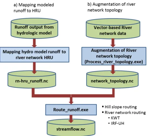
Overall workflow of mizuRoute is illustrated in Fig. 3. There are two main separate data preprocesses before executing the main executable of mizuRoute, route_runoff.exe.

(12)

GMDD

8, 9415–9449, 2015

N. Mizukami et al.

Title Page

Tables Figures

◭ ◮

Back Close

Full Screen / Esc

Discussion

P

a

per

|

Discussion

P

a

per

|

Discussion

P

a

per

|

Discussion

P

a

per

|

to map the runoffoutput from the hydrologic models to the river network HRUs. This process is done by taking the area-weighted runoffof the intersecting hydrologic model HRUs. We developed the python scripts to identify the intersected hydrologic model HRUs for each river network HRU and their fractional areas to the river network HRU area to assist with this process.

5

The second data pre-processing step is augmentation of the river network dataset. Typical topological information in this dataset is the immediate downstream segment for each segment. While a river network can be fully defined based on information about the immediate downstream segment, the river routing schemes in mizuRoute require identification of all the upstream river segments. For this purpose, we have

10

developed a program (process_river_topology.exe) that identifies all the upstream seg-ments for each segment in the river network data based on the information on im-mediate downstream segment. This identification of upstream segments only has to be done once for each unique river network dataset. Therefore, the program (i.e., pro-cess_river_topology.exe) can be used as a preprocessor, which improves the efficiency

15

of the main routing tool, especially when the routing is performed for multiple hydrologic model outputs for a large river system. In addition to the identification of all upstream segments, the topology program identifies upstream HRUs, upstream areas (cumula-tive area of all the upstream HRUs), total upstream distance from each segment to all the upstream segments, etc.

20

5 CONUS-wide mizuRoute simulations

This section demonstrates the capabilities of mizuRoute using the United States Ge-ological Survey (USGS) Geospatial Fabric (GF) vector-based river network (Viger, 2014; http://wwwbrr.cr.usgs.gov/projects/SW_MoWS/GeospatialFabric.html), applied over the contiguous United states (CONUS). The river routing scheme uses both KWT

25

(13)

GMDD

8, 9415–9449, 2015

N. Mizukami et al.

Title Page

Tables Figures

◭ ◮

Back Close

Full Screen / Esc

Discussion

P

a

per

|

Discussion

P

a

per

|

Discussion

P

a

per

|

Discussion

P

a

per

|

scheme and parameters) will differently affect the attenuation of runoff(i.e., the mag-nitude of peak and rate of rising and recession limbs) and the timing of the peak flow. Note that accuracy of the routed flow is not discussed because it depends largely on the accuracy of runoffestimates from the hydrologic model.

5.1 The Geospatial Fabric network topology

5

The GF dataset was developed primarily to facilitate CONUS-wide hydrologic model-ing with the USGS Precipitation RunoffModeling System (PRMS; Leavesley and Stan-nard, 1995). To reduce the computational burden of the hydrologic simulations, the GF dataset is generated by aggregating fine-scale river segments and corresponding catchments or HRUs from the first version of National Hydrography Dataset Plus

(NHD-10

Plus v1; HorizonSystemsCorporation 2010), while still representing small catchments (equivalent in area to 12 digit Hydrologic Unit Code∼100 km2 or smaller basin). The

GF dataset includes line and polygon geometries representing river segments and their catchments, respectively, along with their attribute information including the connectiv-ity between segments (topological information) and their physical attributes such as

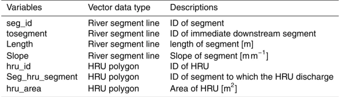
15

channel length, area of the catchment. Table 2 lists the variables of river network vec-tor data necessary for the mizuRoute. The GF dataset (both geometry and attribute in-formation) is stored in Environmental System Research Institute (ESRI) Geodatabase Feature Classes and the topological and physical data (Table 2) in the attribute table is converted to NetCDF format to start with the augmentation of rive network topology

20

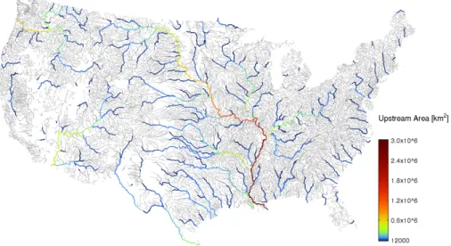
(Fig. 3). The GF dataset include 54 929 river segments and 106 973 catchment HRUs (including the right and left bank of each segment). Figure 4 displays distribution of river segments in the GF vector data. The upstream area of each river segment shown in Fig. 4 is computed based on drainage based HRU (not shown in the Fig. 4) provided in the GF dataset. Although this paper illustrates runoffrouting using GF, the mizuRoute

25

(14)

GMDD

8, 9415–9449, 2015

N. Mizukami et al.

Title Page

Tables Figures

◭ ◮

Back Close

Full Screen / Esc

Discussion

P

a

per

|

Discussion

P

a

per

|

Discussion

P

a

per

|

Discussion

P

a

per

|

5.2 Model setup

We routed the daily runoffsimulations archived by Reclamation (2014) as part of their project “Downscaled CMIP3 and CMIP5 Climate and Hydrology Projections” (http: //gdo-dcp.ucllnl.org/downscaled_cmip_projections/dcpInterface.html). In this project, the VIC model was forced by the spatially downscaled temperature and precipitation

5

outputs at 1/8◦ _{resolution from 97 global climate model outputs from 1950 through} 2099. Additionally, historical runoff simulations were produced at 1/8◦ _{resolution by} the VIC model forced by meteorological forcings from Maurer et al. (2002) from 1950 through 1999 (Maurer et al. data is referred to as M02). The details of the Coupled Model Intercomparison Project Phase 5 (CMIP5) are described by Taylor et al. (2011).

10

First, to use the GF vector-based river network, the 1/8◦gridded runoffwas mapped to each GF HRU by taking areal weighted average of the intersecting area between grid boxes and the GF HRUs.

The routing parameters for each scheme (see Table 1) need to be predetermined. The channel parameters included in the KWT routing method (Manning’s coefficient,n,

15

and river width,w) can be determined by a survey of river channel geometry and river bed condition if the spatial scale of the model domain is very small, but this is usually in-feasible for large spatial domains such as the entire CONUS used here. For the IRF-UH method, the determination of celerity and diffusivity with Eq. (B8) requires information on flow and channel geometry, so for simplicity we follow Lohmann et al. (1996) and

20

treat celerity and diffusivity as parameters. For both schemes, parameter estimation methods need to be developed to determine appropriate values for large-scale appli-cations. For this simulation, the parameter values are determined arbitrarily, with the objective to demonstrate the capabilities of mizuRoute to produce spatially distributed streamflow, not to attain the most accurate simulation.

25

(15)

GMDD

8, 9415–9449, 2015

N. Mizukami et al.

Title Page

Tables Figures

◭ ◮

Back Close

Full Screen / Esc

Discussion

P

a

per

|

Discussion

P

a

per

|

Discussion

P

a

per

|

Discussion

P

a

per

|

(e.g., streamflow gauge location) can be extracted from the NetCDF output file with the ID of the river segment (i.e., seg_id) where the point of interest is located.

5.3 Spatially distributed streamflow in the river network

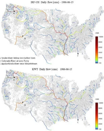
Here we show spatially distributed streamflow estimates using the VIC simulated runoff forced with M02 meteorological data. Figure 5 shows daily mean streamflow estimated

5

with KWT and IFR-UH routing methods for 15 June 1986 as an example. As shown in Fig. 5, both routing schemes produce qualitatively the same spatial pattern of the daily streamflow. From the spatially distributed streamflow time series, point streamflow time series are easily extracted as illustrated in Fig. 6. Figure 6 shows daily streamflow from 1 January 1995 to 31 December 1999 at three locations: (A) Snake River below Ice

Ha-10

bor Dam, (B) Colorado River at Lees Ferry, (C) Apalachicola River near Blountstown. Temporal patterns of flow simulations with the two river routing schemes are very sim-ilar, but the day-to-day differences in estimated streamflow due to the different routing choices become visible.

Another demonstration of mizuRoute’s capability is to produce an ensemble of

pro-15

jected streamflow estimates from the runoff simulations using CMIP5 data. Figure 7 shows the monthly mean of 28 projected streamflow estimates (using CMIP5 RCP 8.5 scenario) at the three locations over three periods: (P1) from 2010 to 2039, (P2) from 2040 to 2069, and (P3) from 2070 to 2099. In this example, the results from the KWT scheme are shown in the Fig. 7. The interpretation of the climate changes impact on

20

the streamflow is not discussed here and complete analyses are left for future investi-gation.

5.4 Sensitivity of streamflow estimates to river routing parameters

Analysis of the sensitivity of simulated hydrographs to channel routing parameters (Ta-ble 1) is performed to examine the e_ffect of parameter values on the streamflow

simu-25

(16)

GMDD

8, 9415–9449, 2015

N. Mizukami et al.

Title Page

Tables Figures

◭ ◮

Back Close

Full Screen / Esc

Discussion

P

a

per

|

Discussion

P

a

per

|

Discussion

P

a

per

|

Discussion

P

a

per

|

runoffwith M02 data and using different river routing parameter values (two parameters for each scheme). We carried out the parameter sensitivity analysis at the three loca-tions in Fig. 6, but found the characteristics of the parameter sensitivity are the same. Therefore, we present the results for Colorado River at Lees Ferry. Figure 8 shows ef-fect of width factorWain Eq. (6) (top panels) and Manning coefficientn(bottom panels) 5

for the KWT scheme. As expected, wider channel width (with largerW_avalue) produces later hydrograph shifts because larger flow area produces slower velocity to conserve the amount of discharge. This effect is enhanced with larger manning coefficientndue to more friction slowing down water flow with larger Manning coefficientn. A similar ef-fect is seen for sensitivity of simulated hydrographs to the Manning coefficientn(bottom

10

panel of Fig. 8).

Figure 9 shows the sensitivity of a simulated hydrograph from 1 October 1990 to 30 September 1991 to the two IRF-UH parameters at Colorado River at Lees Ferry (top panel for sensitivity to celerityC and bottom panel for sensitivity to di_ffusivity D). Interestingly, the effect of diffusivity D is small while celerityCaffects timing of

hydro-15

graph peak. This is because celerityCdirectly changes peak timing without attenuation of IRF, while di_ffusivityDhas little influence on peak timing of IRF although it changes the degree of flashiness (Eq. 12). Due to the low sensitivity of the hydrograph to diff u-sivityD, the degree of hydrograph sensitivity to celerityCis consistent across different di_ffusivity values (bottom panel of Fig. 8).

20

6 Summary and discussion

This paper presents mizuRoute (version 1.0), a river network routing tool that post-processes runo_ffoutputs from any hydrologic or land surface model. We demonstrated the capability of mizuRoute to produce spatially distributed streamflow on a vector-based river network using the USGS GF river network over the CONUS. The

stream-25

(17)

GMDD

8, 9415–9449, 2015

N. Mizukami et al.

Title Page

Tables Figures

◭ ◮

Back Close

Full Screen / Esc

Discussion

P

a

per

|

Discussion

P

a

per

|

Discussion

P

a

per

|

Discussion

P

a

per

|

of the hydrologic simulations, making it possible to produce ensembles of streamflow estimations from multiple hydrologic models. As an example of a practical application of mizuRoute, an ensemble of streamflow projections was produced at USGS gauge points on the river systems across the CONUS from 97 runoffsimulations from Down-scaled CMIP5 Climate and Hydrology Projections (Reclamation 2014). Section 5.3

5

shows some of the streamflow simulations based on the runoff generated with VIC forced by CMIP5 data.

Based on the simulations presented in the Sect. 5.4, the routing parameters can af-fect the simulated hydrograph especially for the KWT method. Though more detailed investigations of those effects need to be performed to fully understand the routing

10

model behaviors, the parameter sensitivity is substantial. More sophisticated methods to estimate routing model parameters need to be developed. River physical parameters are difficult to obtain in a consistent way at the continental scale, but recent develop-ments of the retrieval algorithms for river physical properties (channel width, slope etc.) with remote sensing data are promising (e.g., Pavelsky and Smith, 2008; Fisher

15

et al., 2013; Allen and Pavelsky, 2015), and we expect to see advances in capabilities to estimate the hydraulic geometry of rivers over the coming years (Clark et al., 2015).

Appendix A: Derivation of wave celerity equation used in KWT

The kinematic wave approximation of the full Saint-Venant equations (Eqs. 3 and 4) uses the continuity equation combined with a simplified momentum equation. The

sim-20

plified momentum equation is based on the assumption that the friction slope is equal to the channel slope and that flow is steady and uniform. Under this assumption, Eq. (4) is reduced toS0=Sf. In other words, the gravitational force that moves water downstream

is balanced with the frictional force acting on the riverbed. With this assumption, the dischargeqcan be expressed using a uniform flow formula such as Manning’s

(18)

GMDD

8, 9415–9449, 2015

N. Mizukami et al.

Title Page

Tables Figures

◭ ◮

Back Close

Full Screen / Esc

Discussion

P

a

per

|

Discussion

P

a

per

|

Discussion

P

a

per

|

Discussion

P

a

per

|

tion:

q=Ak nR

α hS

1 2

0 (A1)

wherek is a scalar whose value is 1 for SI units and 1.49 for Imperial units,nis the Manning coefficient,Rhis hydraulic radius [L], which is defined as the cross sectional

flow areaA[L2] divided by the wetted perimeterP [L], and α is a constant coefficient

5

(α=2/3).

We assume the channel shape is rectangular and the geometry is constant through-out one river segment, with widthw,A=wy andP =w+2y. Assuming the channel is wide compared to flow depth (i.e.,w≫y), the hydraulic radiusRhis expressed as

Rh= A P =

wy

w+2y ∼=y (A2)

10

By substituting Eq. (A2) into Eq. (A1), the Manning equation is re-written as

q=wk ny

α+1_S12

0 (A3)

For each stream segment within which the channel widthwis constant, the wave celer-ityCis given by

C=dq dA=

dq

d (wy)∼= dq

wdy (A4)

15

By substituting Manning’s equation (Eq. A3 into Eq. A4), the wave celerity C can be given by

C=(α+1)_·k

n

q

S0·yα (A5)

or expressed as a function of dischargeqas

C=(α+1)_·(w)α−α+1 _·

_k

n

q

S0

_α₊₁1

·q α

α+1 (A6)

(19)

GMDD

8, 9415–9449, 2015

N. Mizukami et al.

Title Page

Tables Figures

◭ ◮

Back Close

Full Screen / Esc

Discussion

P

a

per

|

Discussion

P

a

per

|

Discussion

P

a

per

|

Discussion

P

a

per

|

Appendix B: Derivation of 1-D diffusive equation

We describe in detail the derivation of diffusive wave equations from Saint-Venant equations (Strum, 2001) that are the basis of the IRF-UH method. The development of the IRF-UH method starts with the derivation of the di_ffusive wave equation from the 1-D Saint Venant equations (Eqs. 3 and 4) by neglecting inertia terms (the second term

5

in Eq. 4) and assuming steady flow (eliminating the first term in Eq. 4). The momentum equation (Eq. 4) can therefore be reduced to:

∂y

∂s =S0−Sf (B1)

Now, Manning’s equation can be expressed in terms of channel conveyance,Kc

(car-rying capacity of river channel),

10

q=Kc·

q

Sf (B2)

whereKc=k/n·A·R α

h. SubstitutingSf from Eq. (B2) into Eq. (B1) and differentiating

with respect to time, the momentum equation (Eq. A1) becomes

2q K_c2

∂q ∂t −

2q2 K_c3

∂Kc ∂t =−

∂2y

∂x∂t (B3)

Also, the continuity equation (Eq. 3) can be re-rewritten by differentiating both sides of

15

the equation with respect to distancexas,

∂2q ∂x2 +w

∂2y

∂x∂t=0 (B4)

Combining Eqs. (B3) and (B4) results in

2q K_c2

∂q ∂t −

2q2 K_c3

∂Kc ∂t =

1

w ∂2q

(20)

GMDD

8, 9415–9449, 2015

N. Mizukami et al.

Title Page

Tables Figures

◭ ◮

Back Close

Full Screen / Esc

Discussion

P

a

per

|

Discussion

P

a

per

|

Discussion

P

a

per

|

Discussion

P

a

per

|

Because the channel conveyance,Kc, is a function of flow depth,y, or flow area,A, the

differentiation part of the second term of Eq. (B5) can be written as

∂Kc ∂t =

dKc

dA ∂A

∂t =−

dKc

dA ∂q

∂x (B6)

Finally, inserting Eq. (B6) into Eq. (B5), results in the one-dimensional diffusive wave equation

5

∂q ∂t =D

∂2q ∂x2−C

∂q

∂x (B7)

where

C= q

Kc

dKc

dA =

dq

dA

D= K

2 c

2qw = q

2wS0

(B8)

where parametersCandDare wave celerity [L T−1_{] and di}_ff_{usivity [L}2_T−1_{], respectively.} Here, we assume the flow is uniform (i.e.,Sf=S0).

10

Code availability

The source codes for the river network topology program and the hillslope and river routing along with test data are available along with the user manual on GitHub (https: //github.com/NCAR/mizuRoute). Those codes are developed in Fortran90 and require installation of a NetCDF 4 library (http://www.unidata.ucar.edu/downloads/netcdf/index.

15

(21)

GMDD

8, 9415–9449, 2015

N. Mizukami et al.

Title Page

Tables Figures

◭ ◮

Back Close

Full Screen / Esc

Discussion

P

a

per

|

Discussion

P

a

per

|

Discussion

P

a

per

|

Discussion

P

a

per

|

Acknowledgements. This work was financially supported by the US Army Corps of Engineers’ Climate Preparedness and Resilience programs.

References

Allen, G. H. and Pavelsky, T. M.: Patterns of river width and surface area revealed by the satellite-derived North American River Width data set, Geophys. Res. Lett., 42,

5

2014GL062764, doi:10.1002/2014gl062764, 2015.

Arora, V. K. and Boer, G. J.: A variable velocity flow routing algorithm for GCMs, J. Geophys. Res.-Atmos., 104, 30965–30979, 1999.

Brunner, G. W.: HEC-RAS, River Analysis Ssytem Users’Manual, US Army Corps of Engineers, Hydrologic Engineering Center, 320, 2001.

10

Clark, M. P., Rupp, D. E., Woods, R. A., Zheng, X., Ibbitt, R. P., Slater, A. G., Schmidt, J., and Uddstrom, M. J.: Hydrological data assimilation with the ensemble Kalman filter: use of streamflow observations to update states in a distributed hydrological model, Adv. Water Resour., 31, 1309–1324, 2008.

Clark, M. P.,Fan, Y., Lawrence, D. M., Adam, J. C., Bolster, D., Gochis, D. J., Hooper, R. P.,

15

Kumar, M., Leung, L. R., Mackay, D. S., Maxwell, R. M., Shen, C., Swenson, S. C., and Zeng, X.: Improving the representation of hydrologic processes in Earth System Models, Water Resour. Res., 51, 5929–5956, doi:10.1002/2015wr017096, 2015.

David, C. H., Maidment, D. R., Niu, G.-Y., Yang, Z.-L., Habets, F., and Eijkhout, V.: River Network Routing on the NHDPlus Dataset, J. Hydrometeorol., 12, 913–934 , 2011.

20

Davies, H. N. and Bell, V. A.: Assessment of methods for extracting low-resolution river net-works from high-resolution digital data, Hydrol. Sci. J., 54, 17–28, 2009.

Fekete, B. M., Vörösmarty, C. J., and Lammers, R. B.: Scaling gridded river networks for macroscale hydrology: development, analysis, and control of error, Water Resour. Res., 37, 1955–1967, 2001.

25

(22)

GMDD

8, 9415–9449, 2015

N. Mizukami et al.

Title Page

Tables Figures

◭ ◮

Back Close

Full Screen / Esc

Discussion

P

a

per

|

Discussion

P

a

per

|

Discussion

P

a

per

|

Discussion

P

a

per

|

Gochis, D. J., Yu, W., and Yates, D. N.: The WRF-Hydro model technical description and user’s guide, version 3.0., NCAR Technical Document., NCAR, Boulder CO, 120 pp., 2015. Goring, D. G.: Kinematic shocks and monoclinal waves in the Waimakariri, a steep, braided,

gravel-bed river. Proceedings of the International Symposium on waves: physical and nu-merical modelling, University of British Columbia, Vancouver, Canada, 336–345, 1994.

5

Goteti, G., Famiglietti, J. S., and Asante, K.: A Catchment-Based Hydrologic and Rout-ing ModelRout-ing System with explicit river channels, J. Geophys. Res.-Atmos., 113, D14116, doi:10.1029/2007jd009691, 2008.

HorizonSystemsCorporation: NHDPlus Version 1 (NHDPlusV1) User Guide, available at: http:// www.horizon-systems.com/NHDPlus/NHDPlusV1_documentation.php, (last access: 27

Oc-10

tober 2015), 2010.

Koren, V., Reed, S., Smith, M., Zhang, Z., and Seo, D.-J.: Hydrology laboratory research mod-eling system (HL-RMS) of the US national weather service, J. Hydrol., 291, 297–318, 2004. Leavesley, G. H. and Stannard, L. G.: The precipitation-runo_ff modeling system-PRM S, in:

Computer Models of Watershed Hydrology, edited by: Singh, V. P., Water Resouces

Publica-15

tions, 281–310, 1995.

Lehner, B. and Grill, G.: Global river hydrography and network routing: baseline data and new approaches to study the world’s large river systems, Hydrol. Process., 27, 2171–2186, 2013. Li, H., Wigmosta, M. S., Wu, H., Huang, M., Ke, Y., Coleman, A. M., and Leung, L. R.: A

physi-cally based runoffrouting model for land surface and earth system models, J.

Hydrometeo-20

rol., 14, 808–828, 2013.

Liang, X., Wood, E. F., and Lettenmaier, D. P.: Surface soil moisture parameterization of the VIC-2L model: evaluation and modification, Global Planet. Change, 13, 195–206, 1996. Lohmann, D., Nolte-Holube, R., and Raschke, E.: A large-scale horizontal

rout-ing model to be coupled to land surface parametrization schemes, Tellus A, 48,

25

doi:10.3402/tellusa.v48i5.12200, 1996.

Lohmann, D., Raschke, E., Nijssen, B., and Lettenmaier, D. P.: Regional scale hydrology: I. Formulation of the VIC-2L model coupled to a routing model, Hydrol. Sci. J., 43, 131–141, 1998.

Lucas-Picher, P., Arora, V. K., Caya, D., and Laprise, R.: Implementation of a large-scale

vari-30

(23)

GMDD

8, 9415–9449, 2015

N. Mizukami et al.

Title Page

Tables Figures

◭ ◮

Back Close

Full Screen / Esc

Discussion

P

a

per

|

Discussion

P

a

per

|

Discussion

P

a

per

|

Discussion

P

a

per

|

Maurer, E. P., Wood, A. W., Adam, J. C., Lettenmaier, D. P., and Nijssen, B.: A Long-Term Hy-drologically Based Dataset of Land Surface Fluxes and States for the Conterminous United States, J. Climate, 15, 3237–3251, 2002.

McDonnell, J. J. and Beven, K.: Debates – the future of hydrological sciences: a (common) path forward? A call to action aimed at understanding velocities, celerities and residence

5

time distributions of the headwater hydrograph, Water Resour. Res., 50, 5342–5350, 2014. Miguez-Macho, G. and Fan, Y.: The role of groundwater in the Amazon water cycle: 1. Influence

on seasonal streamflow, flooding and wetlands, J. Geophys. Res.-Atmos., 117, D15113, doi:10.1029/2012jd017539, 2012.

Nijssen, B., Lettenmaier, D. P., Liang, X., Wetzel, S. W., and Wood, E. F.: Streamflow simulation

10

for continental-scale river basins, Water Resour. Res., 33, 711–724, 1997.

O’Donnell, G., Nijssen, B., and Lettenmaier, D. P.: A simple algorithm for generating streamflow networks for grid-based, macroscale hydrological models, Hydrol. Process., 13, 1269–1275, 1999.

Olivera, F., Lear, M. S., Famiglietti, J. S., and Asante, K.: Extracting low-resolution river

15

networks from high-resolution digital elevation models, Water Resour. Res., 38, 1231, doi:10.1029/2001wr000726, 2002.

Paiva, R. C. D., Collischonn, W., and Tucci, C. E. M.: Large scale hydrologic and hydrodynamic modeling using limited data and a GIS based approach, J. Hydrol., 406, 170–181, 2011. Paiva, R. C. D., Buarque, D. C., Collischonn, W., Bonnet, M.-P., Frappart, F., Calmant, S., and

20

Bulhões Mendes, C. A.: Large-scale hydrologic and hydrodynamic modeling of the Amazon River basin, Water Resour. Res., 49, 1226–1243, 2013.

Pavelsky, T. M. and Smith, L. C.: RivWidth: a Software tool for the calculation of river widths from remotely sensed imagery, IEEE Geosci. Remote Sens., 5, 70–73, 2008.

Reclamation: Downscaled CMIP3 and CMIP5 Hydrology Projections – Release of Hydrology

25

Projections, Comparison with Preceding Information and Summary of User Needs, Tech-nical Memorandum No. 86-68210-2011-01, 110 pp., available at: http://gdo-dcp.ucllnl.org/ downscaled_cmip_projections/techmemo/BCSD5HydrologyMemo.pdf, (last access: 27 Oc-tober 2015) 2014.

Reed, S. M.: Deriving flow directions for coarse-resolution (1–4 km) gridded hydrologic

model-30

ing, Water Resour. Res., 39, 1238, doi:10.1029/2003wr001989, 2003.

(24)

GMDD

8, 9415–9449, 2015

N. Mizukami et al.

Title Page

Tables Figures

◭ ◮

Back Close

Full Screen / Esc

Discussion

P

a

per

|

Discussion

P

a

per

|

Discussion

P

a

per

|

Discussion

P

a

per

|

Taylor, K. E., Stouffer, R. J., and Meehl, G. A.: An overview of CMIP5 and the experiment design, B. Am. Meteorol. Soc., 93, 485–498, 2011.

Viger, R. J.: Preliminary spatial parameters for PRMS based on the Geospatial Fab-ric, NLCD2001 and SSURGO, J. Res. US Geol. Surv., available at: http://wwwbrr. cr.usgs.gov/projects/SW_MoWS/GeospatialFabric.html (last access: 27 October 2015),

5

doi:10.5066/F7WM1BF7, 2014.

Wu, H., Kimball, J. S., Mantua, N., and Stanford, J.: Automated upscaling of river networks for macroscale hydrological modeling, Water Resour. Res., 47, W03517, doi:10.1029/2012wr012313, 2011.

Wu, H., Kimball, J. S., Li, H., Huang, M., Leung, L. R., and Adler, R. F.: A new global river

10

network database for macroscale hydrologic modeling, Water Resour. Res., 48, W09701, doi:10.1029/2009wr008871, 2012.

Xia, Y., Mitchell, K., Ek, M., Cosgrove, B., She_ffield, J., Luo, L., Alonge, C., Wei, H., Meng, J., Livneh, B., Duan, Q., and Lohmann, D.: Continental-scale water and energy flux analysis and validation for North American Land Data Assimilation System project phase 2

(NLDAS-15

2): 2. validation of model-simulated streamflow, J. Geophys. Res.-Atmos., 117, D03110, doi:10.1029/2011jd016051, 2012.

Yamazaki, D., Oki, T., and Kanae, S.: Deriving a global river network map and its sub-grid topographic characteristics from a fine-resolution flow direction map, Hydrol. Earth Syst. Sci., 13, 2241–2251, doi:10.5194/hess-13-2241-2009, 2009.

20

Yamazaki, D., Kanae, S., Kim, H., and Oki, T.: A physically based description of floodplain inundation dynamics in a global river routing model, Water Resour. Res., 47, W04501, doi:10.1029/2010wr009726, 2011.

Yamazaki, D., de Almeida, G. A. M., and Bates, P. D.: Improving computational efficiency in global river models by implementing the local inertial flow equation and a vector-based river

25

network map, Water Resour. Res., 49, 7221–7235, 2013.

Yucel, I., Onen, A., Yilmaz, K. K., and Gochis, D. J.: Calibration and evaluation of a flood fore-casting system: utility of numerical weather prediction model, data assimilation and satellite-based rainfall, J. Hydrol., 523, 49–66, 2015.

Zaitchik, B. F., Rodell, M., and Olivera, F.: Evaluation of the Global Land Data Assimilation

Sys-30

(25)

GMDD

8, 9415–9449, 2015

N. Mizukami et al.

Title Page

Tables Figures

◭ ◮

Back Close

Full Screen / Esc

Discussion

P

a

per

|

Discussion

P

a

per

|

Discussion

P

a

per

|

Discussion

P

a

per

|

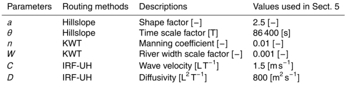
Table 1.Routing model parameters.

Parameters Routing methods Descriptions Values used in Sect. 5

a Hillslope Shape factor [₋] 2.5 [₋]

θ Hillslope Time scale factor [T] 86 400 [s]

n KWT Manning coefficient [₋] 0.01 [₋]

W KWT River width scale factor [₋] 0.001 [₋]

C IRF-UH Wave velocity [L T−1

] 1.5 [m s−1

]

D IRF-UH Diffusivity [L2T−1

] 800 [m2s−1

(26)

GMDD

8, 9415–9449, 2015

N. Mizukami et al.

Title Page

Tables Figures

◭ ◮

Back Close

Full Screen / Esc

Discussion

P

a

per

|

Discussion

P

a

per

|

Discussion

P

a

per

|

Discussion

P

a

per

|

Table 2.River network information required in mizuRoute.

Variables Vector data type Descriptions

seg_id River segment line ID of segment

tosegment River segment line ID of immediate downstream segment Length River segment line length of segment [m]

Slope River segment line Slope of segment [m m−1

] hru_id HRU polygon ID of HRU

(27)

GMDD

8, 9415–9449, 2015

N. Mizukami et al.

Title Page

Tables Figures

◭ ◮

Back Close

Full Screen / Esc

Discussion

P

a

per

|

Discussion

P

a

per

|

Discussion

P

a

per

|

Discussion

P

a

per

|

(28)

GMDD

8, 9415–9449, 2015

N. Mizukami et al.

Title Page

Tables Figures

◭ ◮

Back Close

Full Screen / Esc

Discussion

P

a

per

|

Discussion

P

a

per

|

Discussion

P

a

per

|

Discussion

P

a

per

|

Figure 2.Visualization of waves. The top panel(a)plots a discharge of the wave (cms) against its location (distance (km) from the beginning of the 1st segment) at the beginning of five consecutive time steps. A vertical line indicates the river segment boundary. The bottom panel

(29)

GMDD

8, 9415–9449, 2015

N. Mizukami et al.

Title Page

Tables Figures

◭ ◮

Back Close

Full Screen / Esc

Discussion

P

a

per

|

Discussion

P

a

per

|

Discussion

P

a

per

|

Discussion

P

a

per

|

(30)

GMDD

8, 9415–9449, 2015

N. Mizukami et al.

Title Page

Tables Figures

◭ ◮

Back Close

Full Screen / Esc

Discussion

P

a

per

|

Discussion

P

a

per

|

Discussion

P

a

per

|

Discussion

P

a

per

|

(31)

GMDD

8, 9415–9449, 2015

N. Mizukami et al.

Title Page

Tables Figures

◭ ◮

Back Close

Full Screen / Esc

Discussion

P

a

per

|

Discussion

P

a

per

|

Discussion

P

a

per

|

Discussion

P

a

per

|

(32)

GMDD

8, 9415–9449, 2015

N. Mizukami et al.

Title Page

Tables Figures

◭ ◮

Back Close

Full Screen / Esc

Discussion

P

a

per

|

Discussion

P

a

per

|

Discussion

P

a

per

|

Discussion

P

a

per

|

(33)

GMDD

8, 9415–9449, 2015

N. Mizukami et al.

Title Page

Tables Figures

◭ ◮

Back Close

Full Screen / Esc

Discussion

P

a

per

|

Discussion

P

a

per

|

Discussion

P

a

per

|

Discussion

P

a

per

|

(34)

GMDD

8, 9415–9449, 2015

N. Mizukami et al.

Title Page

Tables Figures

◭ ◮

Back Close

Full Screen / Esc

Discussion

P

a

per

|

Discussion

P

a

per

|

Discussion

P

a

per

|

Discussion

P

a

per

|

(35)

GMDD

8, 9415–9449, 2015

N. Mizukami et al.

Title Page

Tables Figures

◭ ◮

Back Close

Full Screen / Esc

Discussion

P

a

per

|

Discussion

P

a

per

|

Discussion

P

a

per

|

Discussion

P

a

per

|

Figure 9.Sensitivity of simulated runoffat Colorado River at Lees Ferry (Location B in Fig. 4) to IRF-UH parameters. The top panels show sensitivity to diffusivityDwith three fixed celerity

Cvalues (from left to right:C=1.0, 2.0, and 3.0 m s−1