Exact Fill Rates for the (R, S) Inventory Control with Discrete Distributed
Demands for the Backordering Case
Eugenia BABILONI, Ester GUIJARRO, Manuel CARDÓS, Sofía ESTELLÉS Universitat Politècnica de València, Valencia, Spain
[email protected], [email protected], [email protected], [email protected]
The fill rate is usually computed by using the traditional approach, which calculates it as the complement of the quotient between the expected unfulfilled demand and the expected demand per replenishment cycle, instead of directly the expected fraction of fulfilled demand. Fur-thermore the available methods to estimate the fill rate apply only under specific demand conditions. This paper shows the research gap regarding the estimation procedures to com-pute the fill rate and suggests: (i) a new exact procedure to comcom-pute the traditional approxi-mation for any discrete demand distribution; and (ii) a new method to compute the fill rate di-rectly as the fraction of fulfilled demand for any discrete demand distribution. Simulation re-sults show that the latter methods outperform the traditional approach, which underestimates the simulated fill rate, over different demand patterns. This paper focuses on the traditional periodic review, base stock system when backlogged demands are allowed.
Keywords: Inventory, Fill Rate, Periodic Review, Backordering, Discrete Demand
Introduction
The traditional problem of the periodic review, base stock (R, S) system is usually on the determination of the base stock, S, such that total costs are minimized or some target customer service level is fulfilled. Even if the cost criterion is used for that purpose, the service level is usually included by imposing penalty costs on shortages [1] or by using it to compute the base stock in order to mini-mize holding costs of the system [2]. How-ever in real situations these costs are difficult to know and estimate. Particularly difficult is to measure the costs incurred by having in-sufficient stock to attempt the demand since they include such factors as loss of custom-ers’ goodwill [3] [4]. For this reason, practi-tioners use the service level criterion to es-tablish the base stock. Therefore accurate ex-pressions to estimate customer service levels are required. Appropriate service indicators are the cycle service level and the fill rate, being the latter the most used in practice since it considers not only the possibility that the system is out of stock [1], but also the size of the unfulfilled demand when it occurs [5] [6].
This paper focuses on the exact estimation of the fill rate in (R, S) systems. Furthermore, when managing inventories it is required to
know how to proceed when an item is out of stock and a customer order arrives. There are two extreme cases: the backordering case (=any unfulfilled demand is backordered and filled as soon as possible); and the lost sales case (=any unfulfilled demand is lost). This paper focuses on the backordering case. The fill rate is defined as the fraction of de-mand that is immediately fulfilled from on hand stock [7]. Common approach to esti-mate it consists on computing the number of units short, i.e. the demand that is not satis-fied, instead of computing directly the ful-filled demand per replenishment cycle. This approach, known in the related literature as the traditional approximation and denoted by
βTrad further on, consists of calculating the complement of the quotient between the ex-pected unfulfilled demand per replenishment cycle (also known as expected shortage) and the total expected demand per replenishment cycle as follows:
E unfulfilled demand per replenishment cycle 1
total demand per replenishment cycle
Trad
E
(1)
One limitation of the available methods de-voted to estimating βTrad in the (R, S) system
for the backordering case is that they esti-mate it only for specific demand conditions.
In this sense, [3], [8], [9] and [10] suggest methods to estimate it when demand is nor-mal distributed whereas [11], [12], [13] when demand follows any continuous distribution. When demand is discrete, only [3] suggest a method to estimate βTrad for Poisson demands
but to the rest of our knowledge no methods are available to estimate it when demand fol-lows any discrete distribution function and backlog demands are allowed.
Another approach to compute the fill rate consists of directly estimating the fraction of the fulfilled demand per replenishment cycle instead of determining the expected shortage, as follows:
fulfilled demand per replenishment cycle total demand per replenishment cycle
E (2)
However, expression (1) and expression (2) are not equivalent. Note that if X and Y are independent random variables it is true that
E X Y E X E Y and, analogously,
1X
E E X E
Y Y
.
However
1 1
E
Y E Y
and therefore
E X X
E
Y E Y
(see for example [14]). Thus, applying this reasoning to the defini-tion of the fill we find that
fulfilled demand per replenishment cycle fulfilled demand per replenishment cycletotal demand per replenishment cycle total demand per replenishment cycle
E E
E
Since
fulfilled demand per replenishment cycle unfulfilled demand per replenishment cycle 1
total demand per replenishment cycle total demand per replenishment cycle
E E
E E
then
unfulfilled demand per replenishment cycle fulfilled demand per replenishment cycle
1
total demand per replenishment cycle total demand per replenishment cycle
E E
E
[15] proposes methods to estimate both ex-pression (1) and (2) for any discrete demand pattern when inventory is managed following the lost sales case principle. However, there is not available any method to estimate βTrad
and β when demand is modeled by any dis-crete distribution and the inventory is man-aged following the backordering case, i.e. when unfulfilled demand is backlogged to the following cycle. This paper fulfills this research gap and suggests two new and exact methods to estimate both expressions (Sec-tion 3). Furthermore, we present and discuss some illustrative examples of the perfor-mance of both versus a simulated fill rate and over different demand patterns (Section 4).
The discussion and summary of this work are summarized in Section 5.
2 Basic Notation and Assumptions
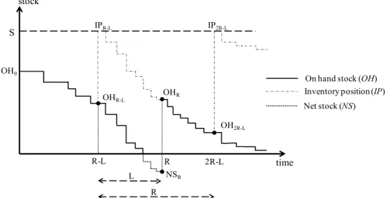
The traditional periodic review, base stock (R, S) system places replenishment orders every R units of time of sufficient magnitude to raise the inventory position to the base stock S. The replenishment order is received
Fig. 1. Example of the evolution of a (R, S) system (backordering case)
Notation in the Figure 1 and in the rest of the paper is as follows:
S = base stock (units),
R = review period corresponding to the time between two consecu-tive reviews and replenishment cycle corresponding to the time between two consecutive deliv-eries (time units),
L = lead time for the replenishment order (time units),
OHt = on hand stock at time t (units),
IPt = inventory position at time t
(units),
NSt = net stock at time t (units),
Dt = total demand during t consecu-tive periods (units),
ft(∙) = probability mass function of Dt,
Ft(∙) = cumulative distribution function of Dt,
This paper assumes that: (i) time is discrete and is organized in a numerable and infinite succession of equi-spaced instants; (ii) the lead time, L, is constant; (iii) the replenish-ment order is added to the inventory at the end of the period in which it is received, hence these products are available for the next period; (iv) demand during a period is fulfilled with the on hand stock at the begin-ning of the period; and (v) demand process is discrete, stationary and i.i.d.
3 Estimation of the Fill Rate in a Discrete Demand Context
3.1 Derivation of an Exact Method to Compute βTrad
The traditional approximation of the fill rate computes the complement of the ratio be-tween the expected unfulfilled demand (ex-pected shortage) and the ex(ex-pected demand per replenishment cycle as shown in expres-sion (1). The expected demand can be straightforwardly computed so all that is left to compute is the expected unfulfilled de-mand per replenishment cycle. Then, if at the beginning of the cycle there is not stock on shelf to satisfy any demand, the net stock at this time is zero or negative (NS0≤0) and therefore the expected shortage is equal to the expected demand during the replenish-ment cycle. Hence, the βTrad is equal to zero.
On the other hand if the net stock at the be-ginning of the cycle is positive (NS0>0), the shortage is equal to the difference between the NS0 and the amount of demand that ex-ceed NS0 during that cycle. By definition, the net stock when positive can be from 1 to S, and hence:
time stock
R-L R
OHR-L
OHR
S
OH0
L
2R-L
OH2R-L
R
NSR
IPR-L IP2R-L
On hand stock (OH)
Inventory position (IP)
0 0
0 0
1 1
unfulfilled demand per replenishment cycle
R
S
R R
NS D NS
E P NS D NS P D (3)
Since the net stock is equivalent to the inven-tory position minus the on order stock, the net stock balance at the beginning of the cy-cle is:
0 L
NS S D .
Then,
0
L 0
L
0
P NS P D S NS f S NS .
Therefore, βTrad when demand follows any discrete distribution function can be estimat-ed with the following expression:
0 0
0 0
1 1
1 1
R
R
S
L R R R
NS D NS
Trad
R R R D
f S NS D NS f D
D f D
(4)
where the denominator represents the ex-pected total demand per replenishment cycle. Note that expression (4) can be used by any discrete demand distribution.
3.2 Derivation of an Exact Method to Compute β
As Section 1 points out, the fill rate is de-fined as the fraction of demand that is imme-diately fulfilled from shelf. From a practical point of view, it is useless to consider a
ser-vice metric when there is no demand to be served. Therefore, cycles that do not show any demand should not be taken into ac-count. According to [15], in order to derive an exact method to compute β over different demand patterns including intermittent de-mand is necessary to include explicitly the condition of having positive demand during the cycle. Then the fill rate can be expressed as
fulfilled demand per replenishment cycle
| positive demand during the cycle total demand per replenishment cycle
E
(5)
Hence, positive demand during a cycle can be: (i) lower or equal than the net stock at the beginning of this cycle, i.e. DR≤NS0, and
therefore the fill rate will be equal to 1; or (ii) greater than the net stock, i.e. DR>NS0, and
therefore the fill rate will be the fraction of that demand which is satisfied by the on hand stock at the beginning of this cycle. There-fore
00
0 0
1
0 0
R
R R R R
D NS R NS
NS P D NS D P D D
D (6)
where the first term indicates the case (i) and the second term indicates the case (ii). Re-writing expression (6) through the probability
mass and cumulative distribution functions of demand, ft(∙) and Ft(∙), respectively, results into
00 0
0
1 0
1 0 1 0
R
R R R R
D NS
R R R
F NS F NS f D
NS
F D F (7)
Therefore, by applying expression (7) to eve-ry positive net stock level at the beginning of the cycle, the method to estimate when
0 0
0 0
0
1 1
0
1 0 1 0
R
S
R R R R
L
NS R D NS R R
F NS F NS f D
f S NS
F D F (8)
4 Illustrative Examples
This section illustrates the performance of expression (4) and (8) (βTradand β
respective-ly) against the simulated fill rate, βSim, which
is computed as the average fraction of the fulfilled demand in every replenishment cy-cle when considering 20,000 consecutive pe-riods (T=20,000) as is expression (9). Data used for the simulation is presented in Table 1 which encompasses 180 different cases.
1
1
T tSim
t t
fulfilled demand
T total demand (9)
Table 1. Set of data (180 cases)
Lead time L = 1, 3, 5
Review period R = 1, 3, 5
Base stock S = 1, 3, 5, 7, 10
Demand Pattern
negative binomial (r,)
smooth (4,0.7); in-termittent (1.25,0.9); erratic (1.5, 0.3); lumpy (0.75,0.25)
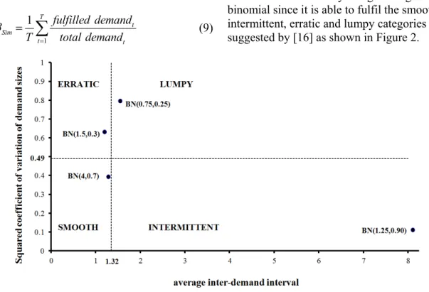
Demand is simulated by using the negative binomial since it is able to fulfil the smooth, intermittent, erratic and lumpy categories suggested by [16] as shown in Figure 2.
Fig. 2. Demand patterns used in the simulation according to the categorization framework of demand suggested by [16]
Figure 3 and Figure 4 show the comparison between βTrad and β versus βSim respectively
for the Table 1 cases. In Figure 3, we see that
βTrad tends to underestimates the simulated
fill rate and therefore the traditional approx-imation seems to be biased. [9] pointed out similar results when demand is normally dis-tributed whereas [15] when demand is Pois-son distributed for the lost sales case. Note that expression (4) leads to the exact value of the traditional approximation. Therefore
Fig. 3. βTrad vs. βSim for the cases from Table
1
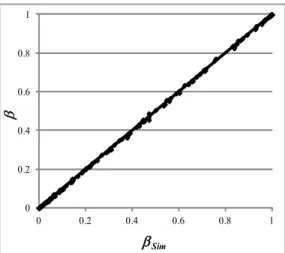
Regarding the performance of β, Figure 4 shows that neither bias nor significant devia-tions appears on it for any of the 180 cases and therefore β computes accurately the fill rate over different discrete demand patterns.
Fig. 4. β vs. βSim for the cases from Table 1
5 Discussion and summary
The traditional approach of the fill rate, βTrad,
computes it by estimating the ratio between the expected unfulfilled demand and the total expected demand per replenishment cycle through computing the expected shortage per replenishment cycle. Section 3.1 presents an exact method to compute βTrad for any
dis-crete demand distribution and for the backordering case. However Figure 3 shows
that βTrad tends to underestimate the
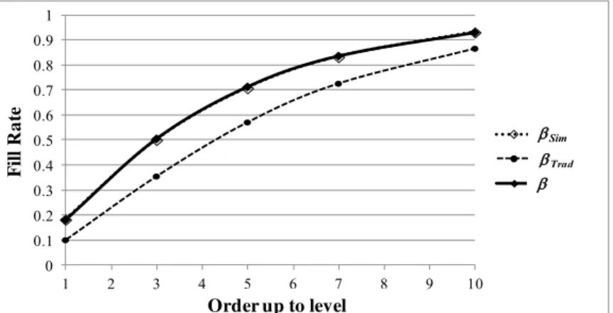
simulat-ed fill rate. An important consequence of the underestimation behavior is found when us-ing a target fill rate to determine the base stock of the inventory policy. Figure 5 shows the evolution of βTrad, βSim, and the exact
es-timation of the fill rate that is derived in Sec-tion 3.2, β, when increasing the base stock for a smooth demand modeled by a negative binomial with r=4 and =0.7. In this case if a target fill rate is set to 0.60, βTrad leads to S=5
whereas in fact just S=3 is necessary to reach the target. In this example, using βTrad to
de-termine base stocks leads to an unnecessary increase in the average stock level and thus the holding costs of the system. This ineffi-ciency is especially relevant in industries in which the unit cost of the item is high and/or storage space is limited. Therefore, managers should be aware of the risk of using the tradi-tional approximation to set the base stock. The method derived in Section 3.2, β, com-putes the fill rate directly as the expected ful-filled demand per replenishment cycle for the backordering case. As Figure 4 shows, this method presents the following advantages: (i) simulation results shows their accuracy over different demand patterns; (ii) outperforms the traditional approach and therefore avoid the above mentioned risks of using βTrad; (iii)
avoids the distortion caused in the metric by the cycles with no demand and therefore can be used even if the probability of no demand during the cycle cannot be neglected; (iv) ap-plies for any discrete demand distribution. Therefore, the exact fill rate method pro-posed in this paper leads to the exact fill rate value when demand follows any discrete dis-tribution and can be applied even when the probability of zero demand cannot be ne-glected. Note that the need to consider only cycles with positive demand does not emerge when using the traditional approximation be-cause it just considers the expected demand, and in the case of no demand cycles it does not affect the estimation.
0 0.2 0.4 0.6 0.8 1
0 0.2 0.4 0.6 0.8 1 Sim
Tr
a
d
0 0.2 0.4 0.6 0.8 1
0 0.2 0.4 0.6 0.8 1 Sim
Fig. 5. Comparison between βTrad, β and βSim with negative binomial demand with r=4 and =0.7 (smooth), R=1 and L=1
This paper is part of a wider research project devoted to identify the most simple and ef-fective method to find the lowest base stock that guarantee the achievement of the target fill rate under any discrete demand context. Therefore, further extensions of this work should be focused on: (i) assessing the exact method when using other discrete distribu-tion funcdistribu-tions of demand; (ii) characterizing the cases where the approximation (including some possible new ones) has the most im-portant deviations; (iii) analyzing risks of us-ing different fill rate approximations to set the parameters of the stock policy and finally (iv) exploring the possibility of embedding results achieved in this work in information systems with the aim of helping decision processes.
Acknowledgments
This work is part of a project supported by the Universitat Politècnica de València, Ref. PAID-06-11/2022.
References
[1] M. C. van der Heijden, "Near cost-optimal inventory control policies for di-vergent networks under fill rate con-straints," International Journal of Pro-duction Economics, vol. 63, no. 2, pp. 161-179, Jan.2000.
[2] E. Babiloni, M. Cardos, and E. Guijarro, "On the exact calculation of the mean stock level in the base stock periodic re-view policy," Journal of Industrial
En-gineering and Management, vol. 4, no. 2, pp. 194-205, 2011.
[3] G. Hadley and T. Whitin, Analysis of In-ventory Systems. Englewood Cliffs, NJ: Prentice-Hall, 1963.
[4] E. A. Silver, "Operations-Research in Inventory Management - A Review and Critique," Operations Research, vol. 29, no. 4, pp. 628-645, 1981.
[5] S. Chopra and P. Meindl, Supply Chain Management, 2nd Edition ed Pearson. Prentice Hall, 2004.
[6] H. Tempelmeier, "On the stochastic un-capacitated dynamic single-item lotsiz-ing problem with service level con-straints," European Journal of Opera-tional Research, vol. 181, no. 1, pp. 184-194, Aug.2007.
[7] H. L. Lee and C. Billington, "Managing Supply Chain Inventory - Pitfalls and Opportunities," Sloan Management Re-view, vol. 33, no. 3, pp. 65-73, 1992. [8] E. A. Silver and R. Peterson, Decisions
system for inventory management and production planning, 2nd ed. New York: John Wiley & Sons, 1985.
[9] M. E. Johnson, H. L. Lee, T. Davis, and R. Hall, "Expressions for Item Fill Rates in Periodic Inventory Systems," Naval Research Logistics, vol. 42, no. 1, pp. 57-80, 1995.
[10]E. A. Silver and D. P. Bischak, "The ex-act fill rate in a periodic review base stock system under normally distributed demand," Omega International Journal
0 0.1 0.2 0.3 0.4 0.5 0.6 0.7 0.8 0.9 1
1 2 3 4 5 6 7 8 9 10
Simulado
tradicional
exacto
Sim
Trad
Order up to level
Fi
ll R
at
of Management Science, vol. 39, no. 3, pp. 346-349, June2011.
[11]M. J. Sobel, "Fill rates of single-stage and multistage supply systems," Manu-facturing and Service Operations Man-agement, vol. 6, no. 1, pp. 41-52, 2004. [12]J. Zhang and J. Zhang, "Fill rate of
sin-gle-stage general periodic review inven-tory systems," Operations Research Let-ters, vol. 35, no. 4, pp. 503-509, Ju-ly2007.
[13]R. H. Teunter, "Note on the fill rate of single-stage general periodic review in-ventory systems," Operations Research Letters, vol. 37, no. 1, pp. 67-68, Jan.2009.
[14]C. M. Grinstead and J. L. Snell, Intro-duction to probability, 2nd ed. United States of American: AMS Bookstore, 1997.
[15]E. Guijarro, M. Cardós, and E. Babiloni, "On the exact calculation of the fill rate in a periodic review inventory policy under discrete demand patterns," Euro-pean Journal of Operational Research, vol. 218, no. 2, pp. 442-447, Apr.2012. [16]A. A. Syntetos, J. E. Boylan, and J. D.
Croston, "On the categorization of de-mand patterns," Journal of the Opera-tional Research Society, vol. 56, no. 5, pp. 495-503, May2005.
Eugenia BABILONI is PhD in Industrial Engineering since 2009. She re-cently becomes assistant professor in the Department of Enterprises Man-agement at the Polytechnic University of Valencia. Her research interests focus on inventory models to forecast and manage items with intermittent demands, either in backordering and lost sales context. She is author of sev-eral book chapters and articles in International Journals in the field of Op-eration research and management.
Ester GUIJARRO has graduated the Faculty of Business Administration and Management in 2007 and she holds an MsC in Financial and Fiscal Management from 2009 from Polytechnic University of Valencia. Currently she is completing her PhD thesis on estimation of the unit fill rate in a peri-odic review inventory policy under discrete demand context. Since 2008 she is lecturer in the Department of Enterprises Management at the Polytechnic University of Valencia. Her research work focuses on inventory manage-ments, more specifically in the categorization of classic inventory control policies via the ap-plication of exact metrics to any given discrete demand context and lost sales scenario.
Manuel CARDÓS holds a PhD in Industrial Engineering since 1985 and he is currently assistant professor in the Department of Enterprises Manage-ment at the Polytechnic University of Valencia, Spain. His research interests focus on supply chain management, scheduling, forecasting and inventory control models, having publishing a considerable number of books and arti-cles in International editorials and Journals.