School of Economics and Management

Carlos Pestana Barros & Nicolas Peypoch

A Comparative Analysis of Productivity Change in Italian and Portuguese Airports

WP 006/2007/DE _________________________________________________________

António Afonso & João Tovar Jalles

The Fiscal-Growth Nexus

WP 01/2012/DE/UECE _________________________________________________________

Department of Economics

W

P

ISSN Nº 0874-4548

School of Economics and Management

The Fiscal-Growth Nexus

António Afonso

and João Tovar Jalles

December 2011

Abstract

We assess the fiscal-growth nexus with a large country panel, accounting for the usually encountered econometric pitfalls. Our results show that revenues have no significant impact on growth whereas expenditures have negative effects. The same is true for the OECD with the addition that government revenue has a negative impact on growth. Taxes on income are usually detrimental to growth, as well as public wages, interest payments, subsidies and government consumption have a negative effect on growth. Social spending is detrimental to growth; spending on education and health boosts growth; and there is weak evidence supporting causality running from expenditures and revenues to output and TFP.

JEL: C23, E62, H50.

Keywords: budgetary decomposition, crises, panel analysis.

_____________________________

* _{The authors are grateful to participants in an ECB seminar for useful comments. Most of the research was conducted while João}

Tovar Jalles was visiting the ECB whose hospitality was greatly appreciated. The opinions expressed herein are those of the authors and do not necessarily reflect those of the ECB or the Eurosystem.

$

ISEG/UTL - Technical University of Lisbon, Department of Economics; UECE – Research Unit on Complexity and Economics. UECE is supported by FCT (Fundação para a Ciência e a Tecnologia, Portugal), email: aafonso@iseg.utl.pt.

#

European Central Bank, Directorate General Economics, Kaiserstraße 29, D-60311 Frankfurt am Main, Germany. email: antonio.afonso@ecb.europa.eu.

+ _{University of Aberdeen, Business School, Edward Wright Building, Dunbar Street, AB24 3QY, Aberdeen, UK. email:}

j.jalles@abdn.ac.uk

#

“…history makes clear that countries that continually spend beyond their means suffer slower growth in incomes and living standards and are prone to greater economic and financial instability. Conversely, good fiscal management is a cornerstone of sustainable growth and prosperity.” Ben Bernanke, Annual Meeting of the Rhode Island Public Expenditure Council, October 4, 2010.

1. Introduction

According to conventional wisdom, in most countries (particularly developing ones), larger

budget deficits have coincided in the past with less efficient government spending, large

bureaucracies, and other counterproductive economic policies. Hence, among the factors that

determine economic growth, government spending and fiscal policies in general are of particular

interest. Such fiscal-growth nexus is particularly important in situations of economic downturns,

where tax revenues tend to flee rather quickly and the spending side of the budget adjusts slowly,

notably in view of the effect of automatic stabilisers and of possible counter-cyclical discretionary

fiscal policies, which implies the building up of larger budget deficits and possible increased fiscal

sustainability problems.

Although large fiscal imbalances can impose an unwarranted burden on the economy, not all

government spending is created equal. Therefore, and in order to inform notably policy decision

making, the effects on economic activity of several spending and revenue budgetary components

need to be assessed, which is the main objective of this paper.

The empirical analysis of the impact of government expenditure on long-run growth include

the early works by Feder (1983), Landau (1983), Ram (1986), Grier and Tullock (1989), Romer

(1990), Barro (1990), Derajavan et al. (1996) and Sala-i-Martin (1997). Such studies used

cross-section data to link measures of government spending with economic growth rates.

However, traditional OLS regression analysis is not sufficient to determine the direction of

causality. When economic growth is regressed on government spending, researchers tend to

interpret this as an eventual confirmation of causality from the latter to the former. Nevertheless, a

significant coefficient can be equally compatible with the Keynesian view (causality from

government expenditure to growth), Wagner’s Law (from growth to spending) and/or a

bi-directional causality between the two variables.

We use cross-sectional/time series data for a large panel of developed and developing countries

for the period 1970-2008. In the empirical estimations of growth specifications we address several

of the econometric caveats that usually plague such analyses: outliers, simultaneity, endogeneity,

cross-sectional dependence, causality, nonlinearities and threshold effects. Specifically, we

examine the following issues: the influence of which budgetary components have a stronger

(TFP) growth rates; the change in coefficient signs (and magnitudes) with different government

debt and budget deficit ratios thresholds; differences in these relationships between country groups

and robustness to different econometric specifications; the direction of causality; is there evidence

in favour of Keynesian (or non-Keynesian) effects or supporting the existence of Wagner’s Law?

Therefore, the contributions of our paper include: i) the assessment of the fiscal-growth nexus

with a diversified variety of methods, providing sensitivity and robustness and dealing notably

with model uncertainty; ii) the study of the relevance of economic and functional government

expenditure categories and of revenue sub-components; iii) panel Granger causality tests, and the

assessment of the existence of cross-sectional dependence within homogeneous groups of

countries.

In a nutshell, our results comprise notably:

i) for the full sample revenues have no significant impact on growth whereas government

expenditures have significant negative effects; ii) the same is true for the OECD sub-sample with

the addition that total government revenues have a negative impact on growth; iii) taxes on income

are usually detrimental to growth; iv) public wages, interest payments, subsidies and government

consumption have a negative effect on output growth; v) expenditures on social security and

welfare are detrimental to growth; vi) both government spending on education and health boosts

growth; vii) there is weak evidence supporting causality running for expenditures or revenues to

GDP per capita (and TFP); viii) there is evidence supporting Wagner’s Law.

The paper is organised as follows. Section two surveys the literature. Section three describes

the analytical and econometric methodology. Section four presents the data and discusses our main

results. Section five summarises the paper’s main findings.

2. Literature

The nexus between fiscal policy and growth has been a subject of several previous studies (see

Zagler and Durnecker, 2003, for a survey). Likewise, Gemmell (2004) has summarised several

empirical work and explains that it is important to distinguish between productive and

non-productive expenditure, and that results depend on whether the simultaneous effects of different

revenue and expenditure categories as well as deficit decisions have been taken into account.

Some pioneer theoretical contributions, underlying our empirical analysis, are notably

Modigliani (1961) and Diamond (1965). For instance, with an endogenous growth model, Cashin

(1994) reports that increased government spending on productive items generate positive

externalities, raising private investment and economic growth. Nevertheless, Slemrod et al. (1995)

theoretical model. This supports the inconclusive results found across the literature and the

debatable nature of the objective impact of fiscal policy on economic growth.

Empirical studies using the economic decomposition of budgetary items usually find evidence

of a negative relationship between government expenditures and growth, such as Barro’s (1997)

seminal contribution in which he found a significantly negative effect on growth from the ratio of

government consumption to GDP. Easterly and Rebelo (1993) take 100 countries from 1970 to

1988 and find that i) there is a strong association between the development level and the fiscal

structure in poor countries relying heavily on international trade taxes, while income taxes are only

important in advanced countries; ii) while the effects of taxation are difficult to isolate empirically.

Lee (1995) found that government consumption was associated with slower growth for a

sample of 89 developed and developing countries for the period 1960-1985. With opposing results,

Slemrod et al. (1995) report a positive correlation between government expenditure to GDP ratio

and the level of real GDP per capita across countries and no relationship for OECD countries

alone. Engen and Skinner (1992) mention that a balanced-budget increase in government spending

reduces output growth in a sample of 107 countries from 1970 to 1985. Landau (1983) and Grier

and Tullock (1989) analyse a sample of 104 and 115 countries, respectively, and find that the

growth of government consumption is negatively correlated with growth, including the OECD.

For 28 OECD countries Afonso and Furceri (2010) report that social contributions, government

consumption and subsidies have a sizeable negative and statistically significant effect on growth.

Romero-Avila and Strauch (2008) conclude for the EU15 countries that the expenditure side of the

budget appears to affect long-run growth over the business cycle. Fölster and Henrekson (1999)

report a tendency towards a negative growth effect of large public expenditures, which is robust

across different econometric specifications. Conte and Darrat (1988) study OECD countries

between 1960 and 1984 and argue that government growth has had mixed effects on growth.

Hakro (2009) finds a positive relationship between government expenditure and GDP per

capita growth for 21 Asian countries, while Bairam (1990) using a sample of 20 African countries

from 1960 to 1985, finds that the effects of government expenditure cannot be generalized.

It is interesting to notice that when it comes to public investment one would expect it to boost

growth. However, in Afonso and Furceri (2010) government investment has a sizeable negative

and statistically significant effect on growth. Devarajan et al. (1996) found that for a sample of 43

developing countries increases in the share of public investment expenditure (including

transportation and communication) have significant negative effects on growth. Prichett (1996)

suggests the so-called “white-elephant” hypothesis in which public investment in developing

developing countries for two distinct time periods (1970-79; 1980-89) and uncover mixed effects

of public investment on growth.

One the one hand, higher public investment raises the national rate of capital accumulation

above the level chosen (in a presumed rational fashion) by private sector agents. Therefore, public

capital spending may crowd out private expenditures on capital goods on an ex-ante basis as

individuals seek to re-establish an optimal inter-temporal allocation of resources. On the other

hand, public capital – particularly infrastructure capital as highways, water systems, sewers and

airports – is likely to bear a complementary relationship with private capital in the private

production technology. Thus, higher public investment may raise the marginal productivity of

private capital and thereby crowd-in private investment (see Afonso and St. Aubyn, 2009).

Slemrod et al. (1995) found a positive correlation between the tax revenue-to-GDP ratio and

the level of real GDP per capita across countries, particularly when developing countries were

included in the sample. Plosser (1992) found a significant negative correlation between the level of

taxes on income and profits (as a share of GDP) and growth of real per capita GDP. Koester and

Kormendi (1989) in a cross-country analysis of 63 countries in the 1970s suggest that apparent

negative effects of taxes on growth disappear upon controlling for potential endogeneity and the

relation between growth and income per capita.

Regarding the functional decomposition of spending, Afonso and Alegre (2011), for a

Euro-area panel between 1970 and 2006, find a significant dependence of productivity on public

expenditure on education, as well as a relevant role of social security and health for economic

growth and the labour market. Folster and Henrekson (2001) report a robust negative relationship

between social expenditures and economic growth. Baum and Lin (1993) taking a heterogeneous

sample of 47 countries find that the growth rate of educational expenditures has a significant

positive impact on growth. The growth rate of welfare expenditures has a negative and

insignificant impact on growth. Differently, Landau (1986) reports that government educational

expenditure has noticeably reduced economic growth.

3. Methodology

3.1. Analytical framework

In the context of a neoclassical growth model the underlying basic aggregate production

function can be written as Y=F(L,K), with Y being the real aggregated output; L the labour force or

Nevertheless, the standard growth model is based on a conditional convergence equation that

relates real growth of per capita GDP to the initial level of income per capita,1 investment-to-GDP

ratio (a proxy for physical capital), a measure of human capital or educational attainment and the

population growth rate, augmented with government expenditures and revenues components.2 As a

result, the aggregate production function is Y=F(L,K,G) being G the relevant fiscal variable.

Therefore the empirical specification to assess the linkages between fiscal policy and growth can

be written as follows:

it i t it it j io

it it

it y y x G

y − ₋₁ =α +β₀ +β₁ +γ +η +ν +ε (1)

where i (i=1,…,N) denotes the country, t (t=1,…,T) indicates the period, yit −yit−1represents the

growth rate of real GDP per capita; y_i0is the initial value of real GDP per capita;3 xjit j=1,2 is a

vector of control variables (x1it comprises of population growth, investment, education and trade

openness; x2it includes x1it – apart from trade openness – and adds labour force participation and

the unemployment rate);4 G_it is a fiscal policy-related variable, either total government revenues

or expenditures (or their respective sub-components5); ν_i, η_tcorrespond to the country-specific

fixed effect and time-fixed effect, respectively. Finally, ε_it is a column vector of some unobserved

zero mean white noise-type satisfying the standard assumptions. α β β, ₀, ₁ and γ are unknown

parameters to be estimated. In addition, and in order to assess an eventual non-linear relationship,

a squared term can also be included for the relevant fiscal variable

3.2. Econometric approaches

Model Selection

Several studies in the growth literature have found a negative bivariate relationship between

growth and a measure of government size (e.g., Plosser, 1993). In addition, it is well known that

the inclusion of particular control variables in a growth regression can wipe out (or change the

signs of) this relationship (Easterly and Rebelo, 1993). Therefore, the motivation for the use of

techniques dealing with uncertainty rests on the concern over the robustness of the candidate

_____________________________

1

The initial level of income per capita is a robust and significant variable for growth (in terms of conditional or beta convergence).

2

Based on the theoretical underpinnings from, e.g., Landau (1983) or Ram (1986). 3

For regressions using annual data, the lagged value of GDP(y_it−1) is used instead. 4

For more details refer to Section 4.1 (“Data and Descriptive Statistics”). 5

variables in any cross-section regression used to explain different success patterns in real income

growth.

With these constraints in mind, we follow Leamer’s (1983) extreme bounds analysis (EBA).

Adapted to our context, this implies the estimation of regressions of the form

ε

+ +

+ +

=aj byjy bzjz bxjxj

Y , (2)

where y is a vector of fixed variables that always appear in the regressions (initial level of income

per capita, investment-to-GDP ratio, population growth and a measure of educational attainment),

z denotes the variable of interest (different components of government expenditure and revenue)

and x_jis a vector of three variables taken from the pool of X additional plausible control variables.

The regression model has to be estimated for the M possible combinations ofx_j ∈X .6 As many

controls are captured by the country dummies we restrict the following ten variables in vector X

(see the Appendix): dependency ratio, fertility, trade openness, labour force, urban population,

unemployment, democracy index, Freedom House composite index, population density and a

measure of financial depth (liquid liabilities over GDP). Therefore, ten conditioning variables

imply 10C₃=120 possible combinations ofx_j∈X .

We also employ the Bayesian Model Averaging (BMA) approach. Essentially BMA treats

parameters and models as random variables and attempts to summarise the uncertainty about the

model in terms of a probability distribution over the space of possible models. The method is used

to average the posterior distribution for the parameters under all possible models, where the

weights are the posterior model probabilities7 (as discussed in more detail in Raftery (1995) and

more recently applied by Malik and Temple (2009)). In the empirical section, the output of the

BMA analysis includes the posterior inclusion probabilities for variables and a sign certainty

index.8 The higher the posterior probability for a particular variable the more robust that

determinant for real GDP growth appears to be.

Panel Techniques

Cross-country regressions are usually based, in this context, on average values of fiscal

variables and growth over long time periods. For instance, for long time spans, the level of

government spending is likely to be influenced by demographics, particularly by an increasing

_____________________________

6

For each model j one estimates zj

b and the corresponding standard deviationσzj. The lower extreme bound is defined as the lowest value of

zj zj

b −2σ and the upper extreme bound is defined to be the largest value ofbzj+2σzj. If the lower extreme bound is negative and the upper extreme bound is positive, the variable is considered not to be robust.

7

To evaluate the posterior model probability the BMA uses the Bayesian Information Criteria (BIC). 8

share of elderly people. Therefore, a simultaneity issue arises. Moreover, problems such as

endogeneity, both in terms of government spending and tax policies, and inefficiency, due to the

discarding of information on within-country variation, can come up.

Resorting to panel data can overcome (some of) these problems, and has other advantages.

Specifically, we focus mainly on combined cross-section time-series regressions using cumulative

5-year non-overlapping averages to smooth the effects of short-run fluctuations, even though

initial growth regressions will be first estimated with annual data. We run within fixed-effects as a

benchmark model despite being aware of the econometric IV-related problems associated with this

method in the context of fiscal policy and growth. Given that technological change occurs over

time, a time index is a logical way to control for the effect of technological progress on the

evolution of per capita GDP growth. However, the effect of technological change on output

growth would likely not be well captured by a simple time trend that assumes a constant effect

over time. Indeed, a Lowess smoothing of per capita GDP against government expenditure and

revenue suggests that there are some non-linear relationships (not shown). Therefore, non-linear

effects of technological change on output growth are allowed for by using individual year indicator

dummies in most estimated panel models.9

Finally, another contribution in our study is the use of two robust estimators, the Method of

Moments (MM)10 and the Least Absolute Deviation (LAD)11 to deal with outliers.

Bias and endogeneity

One needs to address the potential endogeneity problem of right-hand side regressors and

while country-specific fixed effects might capture some of the omitted variables (if we miss out an

important variable it not only means our model is poorly specified it also means that any estimated

parameters are likely to be biased),12 it does not solve the problem and we may get may get biased

_____________________________

9

Since the empirical model assumes that production technology is homogeneous across countries there is nothing inherently inconsistent with the assumption that TFP growth is the same across countries. The period covered by the data includes a number of characteristic slumps (e.g. the two oil crises in the 1970s), but nevertheless one is able to identify a generally upward movement of TFP, particularly in the 1990s.

10

This estimator fits the efficient high breakdown estimator proposed by Yokai (1987), which on the first stage takes the S estimator applied to the residual scale and derives starting values for the coefficient vectors, and on the second stage applies the Huber-type bisquare M-estimator using iteratively re-weighted least squares (IRWLS) to obtain the final coefficient estimates.

11

It minimises the sum of squares over half the observations. The estimator seeks out part of the data for which the model has greatest explanatory power and then bases the parameter estimates on just that portion of the data. We then exclude any observations for which the LAD residual is more than two standard deviations from the mean residual, before re-estimating the model by OLS or FE.

12

coefficient estimates. Therefore, we also use the bias-corrected least-squares dummy variable

(LSDV-C) estimator by Bruno (2005).

Moreover, we use a panel Instrumental Variable-Generalised Least Squares (IV-GLS)

approach, which is then complemented by estimating the main equations using Generalised

Methods of Moments (GMM). The first-differenced GMM estimate can be poorly behaved if the

time series are persistent. This problem can get very serious in practice and authors like Bond,

Hoeffler and Temple (2001) suggest the use of a more efficient GMM estimator, the system

estimator, to exploit stationarity restrictions.13

Hence, we estimate the growth specifications by system-GMM (SYS-GMM) which jointly

estimates the equations in first differences, using as instruments lagged levels of the dependent and

independent variables, and in levels, using as instruments the first differences of the regressors.

Regarding the information on the choice of lagged levels (differences) used as instruments in the

difference (level) equation, as work by Roodman (2009) has indicated, when it comes to moment

conditions more is not always better.14

Panel Granger causality

We also perform a panel version of a Granger-causality test between per capita GDP (and TFP)

and fiscal variables, similarly to Huang and Temple (2005).15 Our TFP variable is a newly

computed measure based on growth accounting techniques according to the methodology

described in Afonso and Jalles (2011).

Since causality can run in either direction, one cannot take government expenditures and

government revenues as strictly exogenous. Alternatively, we run partial adjustment specifications

which allow feedback by means of sequential moment conditions to identify the model (see

Arellano, 2003). The standard approach in the literature would be to specify an AR(1) model as

follows:

1 1 1 1

it it it i t it

y =α y ₋ +β x ₋ +η φ+ +v _{, (3)}

with i=1,2,…N; t=1,2,…,T , and where in our case y_it is real per capita GDP (or TFP) and x_it will

be independent government expenditures and revenues (deflated and in per capita terms). The

_____________________________

13

Although stationarity of averages of investment and population growth rates are quite consistent with the Solow growth model, constant means of the per capita GDP series are clearly not. Fortunately, also here, the inclusion of the time dummies solves the problem without violating the validity of the additional moment restrictions used by the system GMM estimator. In the type of convergence regressions to be analysed, the succession of time dummies can be interpreted as the evolution of common TFP over time.

14

The GMM estimators are likely to suffer from “overfitting bias” once the number of instruments approaches (or exceeds) the number of groups/countries. In the present case, the choice of lags was directed by checking the validity of different sets of instruments and we rely on comparisons of first stage R-squares.

15

reverse relationship is also explored to test notably the hypothesis of the Wagner’s Law holding

for the full sample and OECD sub-sample.

The model in (3) allows for unobserved heterogeneity through the individual effect η_i that

captures the joint effect of time-invariant omitted variables. φ_t is a common time effect, while v_it

is the disturbance term. We also assume that x_it is potentially correlated with η_iand may be

correlated with v_it, but is uncorrelated with future shocks vit+1,vit+2,... The model can be estimated

by difference-GMM (DIF-GMM), which makes use of all available lagged levels of y_it and x_it

dated t-2 (and earlier) as instruments. We use Hansen J's test to assess the model specification and

overidentifying restrictions. As there are a number of limitations of DIF-GMM estimation16, the

system-GMM estimator can be used to alleviate the weak instruments problem. In our setting, the

SYS-GMM uses the standard moment conditions, while SYS-GMM1 (modified 1) only uses the

lagged first-differences of y_it dated t-2 (and earlier) as instruments in levels and SYS-GMM2

(modified 2) only uses lagged first-differences of x_it dated t-2 (and earlier) as instruments in

levels.

In the AR(1) model, one hypothesis of economic interest is the null β₁=0 – this can be

interpreted as a panel data test for Granger causality. Instead of a Wald-type test, we use an

alternative methodology: we estimate both the unrestricted and the restricted models using the

same moment conditions, and then compare their (two-step) Hansen J statistics using an

incremental Hansen test defined as:

)) ( ) ~ (

(J γ J γ) n

D_RU = − (4)

whereJ(γ~)is the minimized GMM criterion for the restricted model, J(γ)) for the unrestricted

model, and n is the number of observations.17

There are some additional issues of interpretation worth discussing in the context of the use of

the above model. One may be interested in the stability of the estimated model. If our model is

stable, we can compute a point estimate for the long-run effect18 of x_it on y_it:

) 1

/( ₁

1 α

β

β_LR = − , (5)

_____________________________

16

For instance, the lagged levels of the series may be weak instruments for first differences, especially when they are highly persistent, or the variance of the individual effects is high relative to the variance of the transient shocks. 17

Under the null, D_RU is asymptotically distributed as χ_r2where r is the number of restrictions. The intuition is that, if the parameter restriction (β1 =0) is valid, the moment conditions should keep their validity even in the restricted model. For more details see Bond and Windmeijer (2005).

18

Lastly, we can test for unobserved heterogeneity. In the absence of individual effects, the

following additional moment conditions become valid, corresponding to the use of lagged-levels

as instruments in the levels equation:

8 ,..., 2 0 )] ( [ 0 )] ( [ 1 1 1 1 1 1 1 1 1 1 = = − − − = − − − − − − − − − t x y y x E x y y y E t it it it it t it it it it φ β α φ β α . (6)

The validity of these additional set of moment conditions (that can be tested using an

incremental Hansen test relative to difference or system GMM), can be evaluated with a test for

the presence of unobserved heterogeneity (where the null is no heterogeneity).19

Cross-sectional dependence

We are aware of the potential issue (in particular, bias in coefficient estimates) induced by a

significant cross-sectional dependence (within similar groups of countries in our sample) in the

error term of the model. As put forward by Eberhardt et al. (2010), the so-called unobserved

common factor technique relies on both latent factors in the error term and regressors to take into

account the existence of cross-sectional dependence. Developed with the panel-data/time-series

econometric literature over the course of the past few years, this method has been largely

employed in macroeconomic panel data exercises (see, e.g., Coakley et al. (2006), Pesaran and

Tosetti (2007), Bai (2009), Kapetanios et al. (2009), Afonso and Rault (2010) and Eberhardt and

Teal (2011 and references therein)). This common factor methodology takes cross-sectional

dependence as the outcome of unobserved time-varying omitted common variables or shocks

which influence each cross-sectional element in a different way. Cross-sectional dependence in the

error term of the estimated model results then in inconsistent coefficient estimates if independent

variables are correlated with the unspecified common variables or shocks.

With this in mind, we test for the presence of cross-sectional dependence Pesaran’s (2004) CD

test statistic based on a standard normal distribution. We then run some of the most important

regression equations with Driscoll-Kraay (1998) robust standard errors. This non-parametric

technique assumes the error structure to be heteroskedastic, autocorrelated up to some lag and

possibly correlated between the groups. Given the particular nature of the dependent variable and

the possibility of error dependence another estimation approach would be worthwhile. We rely on

the Pesaran (2006) common correlated effects pooled (CCEP) estimator, a generalization of the

fixed effects estimator that allows for the possibility of cross section correlation. Including the

(weighted) cross sectional averages of the dependent variable and individual specific regressors is

_____________________________

19

suggested by Pesaran (2009) as an effective way to filter out the impacts of common factors,

which could be common technological shocks or macroeconomic shocks, causing between group

error dependence.

4. Empirical analysis

4.1. Data and descriptive analysis

The dataset was collected from several sources (see Appendix for definitions, acronyms and

sources). Our main dependent variables are: real GDP per capita retrieved from the World Bank’s

Word Development Indicators (WDI); and TFP whose construction is described in Afonso and

Jalles (2011).

Fiscal variables come from the WDI, the IMF’s International Financial Statistics (IFS) and

Easterly’s (2001) data. They comprise the Budget Balance (% GDP) and the Central Government

Debt (% GDP) – the latter retrieved from the IMF’s historical debt database due to Abas et al.

(2010). On the government revenue side we have, as % of GDP: Total Government Revenue, Tax

Revenue, Taxes on Goods and Services, Taxes on Payroll or work force, Taxes on Income, Profits

and Capital Gains, Taxes on Property, and Social Contributions. On the government expenditure

side we consider, as a % of GDP: Total Government Expenditure, Compensation of Employees,

Interest Payments, Subsidies, Public Final Consumption Expenditure, and a functional

decomposition comprising of Spending on Education, Spending on Health, and Spending on

Social Security and Welfare.

With respect to human capital proxies we mainly rely on the average years of schooling for the

population over 25 years old from the international data on educational attainment by Barro and

Lee (2010), but we also take the literacy rate (% of people ages 15 to 24), primary school

enrolment (% gross), primary school duration (years), secondary school enrolment (% gross),

secondary school duration (years), tertiary school enrolment (% gross) and tertiary school duration

(years) from the WDI, for robustness purposes.

As for other controls and regressors, most come from either the WDI or from the IMF’s IFS, as

follows: land area (in square kilometres), population, real interest rate (%), interest rate spread

(lending rate minus deposit rate), imports and exports of goods and services (BoP, current USD),

labour participation rate (% of total labour force), labour force, unemployment, (% of total labour

force), fertility rate (births per woman), urban population (% of total), short-term debt (% of

exports of goods and services), terms of trade adjustment (constant LCU), real effective exchange

rate index (2000=100).

It is also interesting to see how government expenditure and revenue ratios evolved over time.

and revenue have increased throughout time, which implies an increase of the size of the

government notably when trying to provide the additional services related to the welfare state. This

result is particularly clear for the case of government spending, in all country sub-groups.

Figure 1: Kernel Density estimates Expenditures and Revenues (% GDP)

(a) 0 .0 2 .0 4 .0 6 De ns it y

0 20 40 60 80

.

1975-1980 1985-1990

1995-2000 2005-2010

Government Expenditures % GDP

(d) 0 .0 1 .0 2 .0 3 .0 4 De n s it y

0 20 40 60 80

.

1975-1980 1985-1990

1995-2000 2005-2010

Government Revenues % GDP

(b) .0 1 .0 2 .0 3 .0 4 .0 5 De ns it y

10 20 30 40 50 60

.

1975-1980 1985-1990 1995-2000 2005-2010

OECD

Government Expenditures % GDP

(e) 0 .0 1 .0 2 .03 .0 4 .0 5 De n s it y

10 20 30 40 50

.

1975-1980 1985-1990

1995-2000 2005-2010

OECD

Government Revenues % GDP

(c) 0 .0 1 .0 2 .0 3 .0 4 De ns it y

0 20 40 60 80

.

1975-1980 1985-1990 1995-2000 2005-2010 Emerging and Developing

Government Expenditures % GDP

(f) 0 .0 1 .0 2 .0 3 .0 4 De ns it y

0 20 40 60 80

.

1975-1980 1985-1990

1995-2000 2005-2010

Emerging and Developing

Government Revenues % GDP

Source: Authors’ estimates.

4.2. Model selection

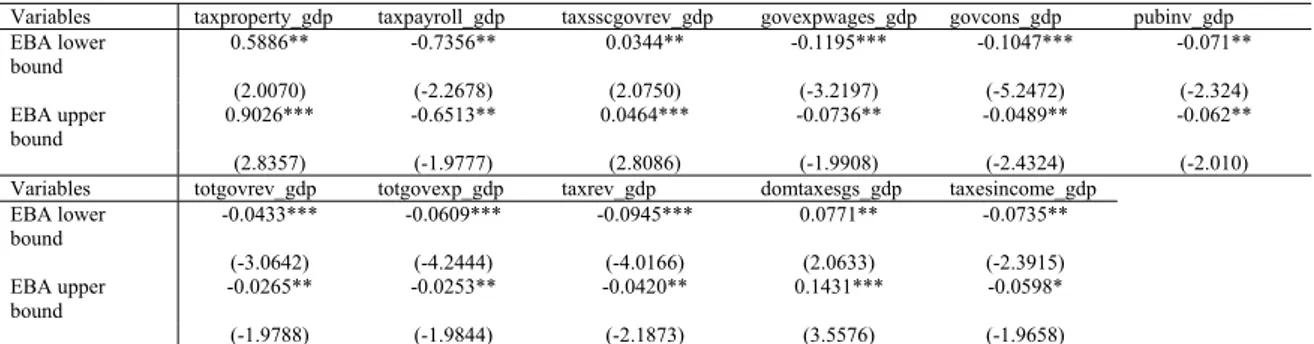
In Table 1 we report our results from the EBA analysis (which controls for collinearity) for the

full sample. The evidence suggests that both total government revenues and expenditures have a

significantly negative impact on output growth (both the upper and lower bounds report the same

sign) and this is in line with Folster and Henrekson (2001) and Afonso and Furceri (2010).

payroll or workforce. Taxes on property, however, seem to boost growth. Turning to expenditures,

public investment has a significantly negative effect on output growth, whereas government

spending on wages of the public sector’s employees and consumption appear to be detrimental to

per capita GDP. We are aware that one of the strongest objections to EBA is that the models

generating the bounds might be flawed (e.g., an important variable may be omitted). Hence, the

results of an EBA should be carefully analysed.

[Table 1]

One reason for the strong appeal of the BMA is that the weights in the final averaging

procedure are tied quite closely to the predictive ability of the different models. Vis-à-vis the EBA,

in the BMA there is no set of fixed variables included and the number of explanatory variables in

the specifications is flexible. In Table 2 we have the results from our BMA application where the

dependent variable is the growth rate of per capita GDP. We present 10 different possible models

containing different sets of regressors grouped by type: scale/size, living conditions,

policy/institutional, education and, finally, government.

A robust result is that the initial level of per capita GDP should be included and it has the

expected negative (and significant) sign, translating the conditional beta-type convergence

hypothesis. Moreover, size, proxied either by population, land area or labour force, is detrimental

to growth. Other interesting results are the fact that both mortality and fertility rates (proxying

living conditions and state of development) have a negative effect on growth. Policy variables such

as openness to international trade have a positive impact on growth, and the same is true with

institutional measures such as the Freedom House index and the Polity democracy index.

Furthermore, we confirm the (positive) impact of human capital, traditionally included in both

theoretical neoclassical and endogenous growth models and seminal empirical studies. With

respect to government-related variables the main findings are: i) inconclusive results for the effects

of government revenues attested by mixed evidence from models 5 and 10, and a negative impact

of government outlays. Evidence seems to suggest that both the debt-to-GDP ratio and debt

average term to maturity negatively affect growth.

[Table 2]

We then take a similar approach and set of regressors to study their impact on TFP growth and

on the stock of capital per worker growth (see Afonso and Jalles, 2011). Some results worth

highlighting are the following. We observe that education matters positively to TFP growth as well

as government revenues and expenditures, while debt has a detrimental effect. The same applies to

Finally, in Table 3 for each dependent variable previously discussed we report the top models

based on their R-squares. All in all, the best models include expenditure components and signal

the relatively less important impact/effect attributed to government revenues’ categories.

[Table 3]

4.3. Fiscal-growth relationship

According notably to Gupta et al. (2005) the composition of public outlays has a bearing on

the nexus between budget deficits and growth. Table 4 summarizes the results of a series of panel

regressions of per capita GDP growth on four variables: total government expenditures (% GDP),

total government revenues (% GDP) and their growth rates, using 5-year averages. When

expenditure is included alone in the equation, the correlation between government size and growth

is negative and significant at the 1 percent level. Government revenue appears with a negative,

though insignificant, coefficient when included alone (specification 3). However, initial

government revenues are strongly correlated with initial income per capita (specification 11), a

variable which is itself negatively correlated with growth (specification 1). Hence, total

government revenue could be capturing part of the effect of initial income when we omit this

variable from the equation. Even after controlling for initial income, the coefficient of total

government revenue remains negative and insignificant. The expansion of government revenues,

rather than its absolute size, seems to boost growth (specifications 5 and 9). If instead of

fixed-effects we accounted for endogeneity problems and ran an IV-GLS regression results don’t

change.

[Table 4]

Results for the OECD sub-sample (available from the authors) show that both expenditures

and revenues appear with statistically significant negative coefficients in almost all regressions.

Moreover, and even if both variables are strongly correlated with initial income per capita, after

controlling for initial income, we still get the same result. The coefficients of total government

revenue and expenditure are negative and significant. Contrary to the full sample case, government

revenue growth is detrimental to economic growth. The same is true for spending growth

(previously insignificant for the full sample).20

Taking the “standard” regressors usually present in growth regressions – initial per capita

GDP, population growth, trade openness, education and private investment – we explore how

sensitive are total government expenditures and revenues when included together with this

variable set. Table 5 shows that total government expenditures have a negative and statistically

significant effect on output growth for the entire sample as well as for the OECD and emerging _____________________________

20

economies sub-groups when fixed-effects estimation is carried out. For emerging countries,

government revenues have a detrimental effect to growth.21 Making use of outlier-robust LAD and

MM techniques does not alter our results22, nor if one controls for endogeneity issues with panel

IV-GLS, DIFF-GMM and SYS-GMM. Therefore, the statistically significant negative coefficient

of total government expenditures is robust across econometric specifications, whereas less clear

results (insignificance) are attributed to the effects of government revenues on output growth. As

an additional robustness exercise, conducting the same analysis with annual data instead doesn’t

alter qualitatively our previous findings.

[Table 5]

4.3.1. Budgetary Economic Decomposition

In order to assess the impact of different budgetary sub-components on output growth, we

estimate the following baseline specification:

1 1 0 0 1

it it it i it it t i it

y −y − =α +β y +βZ +γF + + +η ν ε (8)

where y_it −y_it−1represents again the growth rate of real GDP per capita, and y_i0is the initial value

of the real GDP per capita. Z1it is a vector of control variables; F_it is a vector of budgetary

component(s) of interest, either from the expenditure or revenue side); ν_i, η_tcorrespond to the

country-specific fixed effect and time-fixed effect, respectively. Finally, ε_it is some unobserved

zero mean white noise-type column vector satisfying the standard assumptions. α,β₀,β₁,γ are

unknown parameter vectors to be estimated. Z1it includes labour force participation rate,

population growth, education, private investment.

We know that a typical business cycle correlation might imply that when growth falls,

government expenditure increases and tax revenues would typically decrease. Furthermore, an

expansionary fiscal policy can stimulate aggregate demand and thus growth. To check the

importance of these correlations a control variable unemployment has been included in the model,

because it is the variable that mostly varies with the business cycle.

Given our benchmark equation (8) together with its respective set of controls, we now move to

the inclusion of different sub-components of government revenues and expenditures. In Table 6

(panel A) we include each item, one at a time.

[Table 6]

_____________________________

21

Running an IV-GLS estimator enforces our results and increases the magnitude of the coefficient estimates. 22

Inspecting first the revenues’ (panel A1) we observe that each component does not

significantly affect growth in OECD countries. However, domestic taxes on goods and services

have a positive effect on output growth for the full sample and emerging economies sub-group, but

not for the OECD. This may seem counterintuitive, but Helms (1985) and Mofidi and Stone

(1990) found that taxes spent on publicly provided productive inputs tend to enhance growth.23 For

the emerging economies group, taxes on income, profits and capital gains have a statistically

significant negative impact on growth, whereas taxes on payroll or workforce has a reverse effect.

24

Turning to the expenditure side (panel A2), final government consumption has a significantly

negative effect on output growth for the full and OECD samples. Indeed, economic theory

suggests a variety of explanations for the negative relationship between government spending and

growth. First, government spending can crowd out private spending.25 Second, the level of

government spending may proxy other government intrusions into the workings of the private

sector, especially regulations which restrain economic growth and efficiency. Empirically, our

results are in line with the works by Landau (1983, 1986), Grier and Tullock (1989), Barro (1991),

Barro and Sala-i-Martin (1995), who have found a negative effect of government consumption on

growth.

Still in Table 6 (panel A), for the OECD sub-group, apart from public investment, which

appears with a positive but insignificant coefficient, all remaining spending components adversely

affect growth, in particular expenditures with wages and consumption spending. For the full

sample and emerging economies sub-group, public investment appears with a significantly

negative coefficient. Possibly inefficient and bureaucratic public sectors may generate lobbying,

rent-seeking and other non-productive outcomes and activities that erode potentially the positive

contribution coming from such investment. This is also in line with the literature reviewed before

(notably Devarajan et al., 1996, and Prichett, 1996).

In addition, we observe that interest payments and subsidies have a negative effect on GDP per

capita growth, the latter eventually due to the fact that it creates deadweight loss inefficiencies

when distorting the market from its own natural equilibrium.26

_____________________________

23

Theoretically, in Barro-style models, increases in taxes can enhance, have no effect or impede growth depending, in particular, on the initial level of taxes as well as how revenues are spent.

24

Most growth models predict that taxes on investment and income have a detrimental effect on growth. These taxes affect the growth rate through a direct channel, reducing the private returns to accumulation. On empirical grounds, the effects of taxes on growth are not so clear and most research has focused on OECD countries.

25

In theory, government expenditure can be allocated to growth enhancing infrastructure and education but outlays also go for redistribution or government-mandated consumption, which does not improve productivity.

26

As a next step we include all components of each budgetary block simultaneously in regression

(8). Table 6, Panel B, reports the results for both the revenue and expenditure blocks. As when

included individually, domestic taxes on goods and services appear with a statistically significant

positive coefficient in the growth regression. Regarding taxes on income, profits and capital gains,

the negative significance is absent in the emerging economies sub-group, but it is present for the

full sample. As regards the OECD sub-group, revenue variables are never significant in per capita

GDP growth equations.

Taking account of endogeneity problems (with a corresponding panel IV-GLS approach – not

shown) increases the significance level in most coefficients, in particular the basic set of controls

(negative effect of unemployment for both the full and OECD samples; negative effect of

population growth. Most revenues’ coefficients for the OECD sub-group remain insignificant.27

Regarding the expenditure items in Panel B2, on average, the R-squares are somewhat higher

than when disaggregated revenues are included in the regressions. Overall, evidence suggests a

higher importance attributed to government expenditures than to revenues. Apart from expected

signs on the basic set of controls as already discussed, a closer inspection indicates that wage

spending keeps its negative impact on growth equations, similarly as to when it is included

individually in the regression, although not statistically significant. Government final consumption

expenditure is detrimental to growth. As with the case of government revenues, when endogeneity

is taken into account, most coefficients increase their significance levels with “right” sign

estimates. Moreover, R-squares increase from FE to IV-GLS estimation in every specification.

4.4. Functional spending

Government spending can play an essential role in economic development by maintaining law

and order, providing economic infrastructure, harmonizing conflicts between private and social

interests, increasing labour productivity through education and health and enhancing export

industries. Hence, in terms of the functional decomposition of government expenditures, we

differentiate the effects from spending on education, health, and social security (and welfare),

which constitute the main items of government spending.

In Table 7, Panel A, each of the above spending categories is included in the regression one at

a time. For reasons of parsimony we do not report the full set of coefficient estimates. Regarding

social security spending, it has a statistically negative effect on growth in the OECD sub-group.

Taxes on income become statistically significant and negative in specification 1, thereby adversely affecting output growth. On the expenditure side results are kept qualitatively unchanged.

27

This is in accordance with e.g. Landau (1983, 1986), Barro (1991) and Grier and Tullock (1989)

who found a negative relationship between social expenditures and growth.

In Panel B, the three variables of interest are included simultaneously in each regression. In

Panel B, the same conclusions apply with the addition that government expenditure on education

now affects positively growth in the emerging economies sub-group. It has been argued that

investment in human capital like education (Barro and Sala-i-Martin, 1995) and health (Devarajan

et al., 1996) has positive effects on growth.

[Table 7]

4.5. The cyclicality of functional spending

The cyclicality of government expenditure is also an important issue, notably from a policy

making perspective. Therefore, we assess the cyclicality of the three sub-categories previously

discussed: education, health, and social security and welfare spending. Changes in expenditure

patterns may arise from discretionary actions by policy makers or from the operation of automatic

stabilizers (see notably Granado et al., 2010). Our analysis is an encompassing one since we i)

consider, besides education and health, also government expenditure on social security and

welfare,28 ii) and use a substantially large time span (1970-2008).

Most studies find that fiscal policy is procyclical in developing countries and countercyclical

or acyclical in advanced ones.29 A number of explanations have been put forward to justify the

different cyclical pattern in different groups of countries (see, Tornell and Lane (1999) or Gavin

and Perotti (2007) for review). With this in mind, we transform our spending variables into log

levels, deflated with the CPI at 2000 prices (which matches the same reference year for real GDP).

Following the literature we estimate:

0 1 1 2

it it it it it t i it

EXP =α +βY +βBB − +βTOT + + +η ν ε (9)

where EXP_it is the change in the real value of the log of the expenditure item of interest and Y_it is

the real GDP growth rate. BB_it−1 is the government’s budget balance (% GDP), which captures the

potential effect of borrowing constraints on public spending. Countries with high initial budget

deficits are perceived to be at a greater risk of debt default and as a result have a lower access to

capital markets during recessions. They would be expected to exhibit a higher degree of

pro-cyclicality. TOT_it is an index (its change) of the country’s terms of trade.30 The remaining usual

_____________________________

28

These three functional spending categories accounted for 41.6%, 54.7%, and 34.5% of government spending, respectively in the full, OECD and developing country-group over the full time span considered in our sample.

29

See, inter alia, Tornell and Lane (1999), Alesina and Tabellini (2005) and Ilzetzki and Vegh (2008). 30

assumptions apply, in particularν_i and η_t are country specific and time effects – the latter to

control for global shocks.β₀ is the parameter of interest, measuring the degree of cyclicality: a

positive estimate implies a pro-cyclical behaviour; a negative one indicates a countercyclical

behaviour of the respective spending items.

The potential endogeneity is taken care by running SYS-GMM with appropriate lags of the

regressors used as instruments.31 We first estimate (9) without control variables using annual data

for the full, OECD and Emerging and Developing (E+D) samples (not shown). Most GDP growth

coefficients are statistically insignificant for all four spending categories, apart from evidence of

countercyclical total government expenditures attributed to the OECD sub-group (which is in line

with the literature) and a countercyclical pattern for expenditures in social security and welfare in

the different samples, in line with Hallerberg and Strauch (2002) and Darby and Melitz (2008). In

Table 8 we report estimated coefficients now with the full control set included. For the OECD the

government expenditure coefficient remains significant. Moreover, we keep the countercyclical

result for spending on social security and welfare (for both the full and OECD samples).

[Table 8]

Given that public expenditures may respond asymmetrically during good and bad times, we

test this hypothesis by accounting for so-called good and bad times. Therefore, we define good

times as those in which the output gap is positive and bad times when the output gap is negative.32

Our results suggest that for the OECD group total government expenditure is countercyclical in

both good and bad times, with the coefficient in bad times being 50% larger in absolute value

(more negative). We keep the acyclicality result for education and health expenditures, and the

countercyclical result for spending in social security and welfare is also maintained. In fact, in

good times the estimated coefficient for social security spending is larger in magnitude (more

negative). For emerging and developing countries our results are in line with Jaimovich and

Panizza (2007) who report that after controlling for endogeneity, total government spending is

acyclical in both good and bad times.

All in all, most spending items are acyclical, with the exception of total expenditures and

spending on social security and welfare where evidence points to counter-cyclicality, particularly

in OECD countries.

_____________________________

31

Fixed effects estimation results are available from the authors upon request. 32

4.6. Non-linearities in budgetary decomposition

An additional exercise is to further explore possible effects coming from non-linearities in the

context of the budgetary decomposition. The results in the previous sections suggest that the

reduction of budget deficits can be conducive to higher growth. Of interest is whether these results

hold for all countries (and sub-groups) in the sample(s), in particular, for countries that have

already achieved a modicum of macroeconomic (fiscal) stability.33 Therefore, we spit the

sample(s) into countries labelled “above” or “below”, based on a given fiscal threshold.

Specifically, an “above” type country is defined as a country that maintained on average (over

time) a budget deficit below 3% of GDP. Conversely, a “below” type country is such that it

maintained an average budget deficit above 3% of GDP.34 We also repeat the procedure with a

60% of GDP government debt threshold (that is, the “above” type country is one that maintained

an average debt ratio below 60% of GDP over the period; mutatis mutandis for the “below”

case).35

In Table 9 we report the results with the 3% deficit threshold. Needless to say that some of

these results require care in interpretation given the truncated nature of the resulting sample and

reduced number of available observations. First, both the unemployment rate and the dependency

ratio appear with a negative and statistically high coefficient in several regressions.

In the fixed-effects specifications 7-12 for the revenue panel both in the full sample and in the

emerging economies sub-group, some points are worthwhile emphasizing. Apart from retaining

the positive coefficient on domestic taxes on goods and services that we have commented on

before, the case of the below 3% threshold, for the full sample, now registers a statistically positive

coefficient on the contributions to social security, which previously where insignificant (but

positive still) in Table 6. For the case above 3%, the emerging economies sub-group retain the

statistically negative impact of social security contributions allocated in Table 6 for the entire

emerging group (though now with an increased magnitude of the estimate). For this group of

countries, taxes on income, profits and capital gains is detrimental to growth in the below 3%

deficit set of economies.

_____________________________

33

On the same line see, e.g., Gupta et al. (2005). 34

The 3% value is an ad-hoc number stemming from the European Union Stability and Growth Pact (SGP) rationale. For the OECD sub-group, countries classified as being “above” average, lower deficits, are: Australia, Canada, Czech Republic, Denmark, Finland, France, Germany, Iceland, Korea, Luxembourg, Netherlands, New Zealand, Norway, Poland, Slovakiam Spain, Switzerland, UK and US. The “below” average ones, higher deficits, are: Austria, Greece, Hungary, Ireland, Italy, Japan, Mexico, Portugal, Sweden and Turkey.

35

Furthermore, for the OECD sub-sample, coefficient estimates which were entirely insignificant

in Table 6 now appear with statistically meaningful coefficients. Moreover, it is interesting to

observe that depending whether we take the below or above 3% threshold set of economies,

coefficient signs may be reversed (e.g., negative impact of taxes on income, profits and capital

gains as well as taxes on payroll or workforce for the above 3% group, but positive ones for the

below 3% group). For instance, this can imply that with higher fiscal imbalances, additional taxes

on income depress growth.

Third, for the expenditure set of regressions, results are less controversial or dubious in their

“expected” or “right” coefficient signs. As before, we have negative effects of government

spending on wages, final consumption and public investment (the latter notably for the emerging

economies sample, regardless of the deficit threshold).

As a robustness exercise we have conducted a sensitivity analysis based on the exclusion of

labour force participation, unemployment and dependency ratio (not shown). Whereas coefficients,

magnitudes and statistical significance levels in the expenditure-based regressions are kept

unchanged, the same does not apply to specifications 7-12, concerning revenues. In particular, we

lose significance in all revenue components for the OECD below 3% sub-group (the results of

Table 6). For the OECD above 3% case, domestic taxes on goods and services have a statistically

negative coefficient and taxes on property a statistically positive coefficient, both of which were

absent before (we loose significance on the remaining variables) though. All in all, results with

revenue components are sensitive to the inclusion/exclusion of particular controls, and hence

should be interpreted with care.

Finally, we have redefined our deficit threshold such that now instead of averaging over the

countries time span, we take each 5-year average period to assess/determine the above and below

3% classification. Moreover, as before but now based on the new criterion, we did the analysis

with the labour force participation, unemployment and dependency ratio excluded from the set of

regressors. Reporting all these would lead us far off-track. A typical result is the confirmation that

government expenditures’ components are generally detrimental to growth irrespectively of the

country group and deficit threshold classification. As for revenues’ components, results are mixed,

unclear or contradictory depending on the set of regressors included, geographical sample and

deficit rule used.

[Table 9]

As described above we also used a 60% threshold for the average public debt-to-GDP ratio

over a country’s time series span. For reasons of parsimony results are available upon request.

Overall, we get mixed evidence from revenues’ components coefficient estimates. As for the

appear with statistically significant negative signs. Redoing these estimations with the truncated

set of basic regressors or using the 5-year average period debt-rule instead of the country average,

doesn’t alter the main results (not shown).

Figure 2 summarizes the relationship between output growth, government debt-to-GDP ratio

and the budget balance ratio according to the 3% (60%) fiscal thresholds classification. The pattern

arising is that countries with average lower debt ratios and with lower budget deficits are

associated with higher GDP real growth rates.

Figure 2: “Above” and “Below” Average Performers, pc GDP growth, budget and debt ratios

2.5

2.0 2.6 1.9

-0.8 -6.0 -2.1 -3.7 0.0 10.0 20.0 30.0 40.0 50.0 60.0 70.0 80.0 90.0 100.0

Above Av. (-3%) Below Av. (-3%) Above Av. (60%) Below Av. (60%)

%G D P -7.0 -6.0 -5.0 -4.0 -3.0 -2.0 -1.0 0.0 1.0 2.0 3.0 4.0 % (f or G D P p c g row th ) % G D P ( for bu dg e t b a la nc e )

Gov.Debt (%GDP) GDPpc growth (%) Budget Balance (%GDP)

Source: Authors’ estimates.

4.7. Panel Granger-causality tests

It is also important to understand whether expenditures (revenues) Granger cause per capita

GDP (and TFP), or the reverse applies or even if one finds two-way bidirectional causality. In

previous studies, Hakro (2009) finds evidence suggesting that government expenditures are growth

inducing, and a larger size of the government will certainly create opportunities of employment

and hence growth, and subsequently higher income per capita. In a related sample Kumar (2009)

infers instead that Wagner’s Law does hold.36 Yuk (2005) takes a long term perspective on UK

time series and, although support for Wagner’s Law is sensitive to the choice of the sample period,

there is evidence that GDP growth Granger-causes the share of government spending in GDP.

Loizides and Vamvoukas (2004) using a bivariate ECM conclude that government size Granger

causes economic growth in all countries in the short and long run; economic growth Granger

causes increases in the relative size of government in Greece, and when inflation is included, in the

UK.

_____________________________

36

We find little evidence of robust Granger causality from per capita GDP to government

expenditure37 across econometric specifications, with only one model indicating a negative short

and long-run effect of total government expenditure on output growth.

However, there is stronger evidence supporting the reverse relationship, that is, from GDP to

expenditures, therefore favouring the idea of Wagner’s Law. In particular, there are significant

short and long-run effects, we reject the null of no Granger-causality using our two-step Hansen

incremental test, and diagnostics are well behaved (Table 10).38

[Table 10]

With respect to causality running from government expenditures to TFP we find evidence

supporting it, together with positive and significant short and long-run coefficients. For the OECD

sub-group results are similar (not shown).

4.8. Cross-sectional dependence

As discussed in Section 3 it is natural to suspect about the existence of cross-sectional

dependence across homogeneous groups of economies. Therefore, we use Pesaran’s CD test39 for

the OECD sub-samples and we find a statistic of 15.26, corresponding to a p-value of zero (the

null hypothesis is cross-sectional independence).

In Table 11 we run benchmark type growth regressions for this OECD sample using both a

Driscoll-Kraay robust estimation approach and the Pesaran’s Common Correlated Effects Pooled

Estimator (CCEP). We restrict ourselves to the examination of seven main variables of interest:

total government expenditures and revenues (% GDP), their respective growth rates, and the

functional decomposition of government expenditures (education, health, and social security and

welfare). Similarly to our earlier results we find negative and statistically significant coefficients

for the effect of total government expenditures and revenues on output growth (the latter only true

when running the Driscoll-Kraay regression). We find a negative effect of revenues’ growth rate,

confirming previous results. As for specifications 5 and 10 both government spending on

education and health yield insignificant coefficients, though social security spending yields a

statistically negative coefficient – reinforcing our previous results.

[Table 11]

_____________________________

37

Both total government expenditures and revenues (% GDP) were converted to nominal levels, deflated using the CPI and scaled by population. Hence, we have real GDP per capita and either real total government expenditures or revenues in per capita terms as well (so that both variables of interest are comparable).

38

Redoing the analysis for the OECD sub-sample (not shown), we get slightly stronger results favouring Granger causality from government spending to GDP for a positive short-run effect in 3 out of 6 models. Nevertheless, there does not seem to be a significant long-run effect. For the OECD the reverse relationship still holds with evidence of Granger-causality from GDP to government spending, as well as positive and significant short and long-run effects in both the pooled OLS and FE models.

39