JOINT OPTIMIZATION OF NEW PRODUCTION, WARRANTY SERVICING STRATEGY AND SECONDARY MARKET SUPPLY
UNDER CONSUMER RETURNS∗
Marc Reimann
1∗∗and Weihua Zhang
2Received November 6, 2013 / Accepted November 9, 2013
ABSTRACT.In this paper, we consider an OEM selling new products to the market offering (i) a warranty period during which defective units are dealt with at no cost for the customer, and (ii) a full refund to customers who return products that do not meet their expectations (consumer returns). The manufacturer has different options for satisfying the warranty cases as well as for utilizing the consumer returns. Warranty cases could be dealt with by repairing the defective units, replacing them with new products, or replacing them with refurbished consumer returns. Alternatively leftover new products or consumer returns can also be sold on a secondary market. We develop a model and derive the OEMs optimal decisions with respect to these options under demand uncertainty on the primary market.
Keywords: warranty returns, consumer returns, refurbished products, secondary market, warranty servic-ing, newsvendor approach.
1 INTRODUCTION
In many industries companies have been experiencing increasing competitiveness for many years. In order to survive under such conditions firms have implemented various strategies for attracting new customers as well as keeping and satisfying existing customers. These strate-gies include generous warranty agreements to deal with product defects as well as money-back-guarantees (MBGs) to deal with buyer’s remorse. Different car manufacturers offer warranty contracts including the availability of original spare parts for a time horizon of more than 15 years (seee.g.http://www.volkswagen.de/de/servicezubehoer/VolkswagenOriginalTeile/original teile.html). Leatherman offers a 25-year guarantee for its tools (http://www.leatherman.com/sup-port/nawarranty). Amazon.com offers a full MBG within 30 days of purchase (http://www.ama-zon.com/gp/help/customer/display.html?nodeId=15015721), while IKEA targets customer
satis-∗Invited paper ∗∗Corresponding author
faction with a 100 day full refund policy (http://www.ikea.com/ms/en SG/customer service/re-turn policy/)3.
However, these policies increase the number of returns drastically. Recent studies find that re-turns constitute up to 35% of sales quantities (seee.g. [7]). Thus, companies need to carefully plan their operations associated with these warranty and consumer return schemes, including coordination with the forward production and sales processes.
Different companies use different strategies towards satisfying warranty claims. While some original equipment manufacturers (OEMs) repair all defects occurring during the warranty pe-riod, others offer replacement with new units. A third strategy is to utilize used and returned products for dealing with warranty cases (c.f.e.g. [18]). This third strategy also provides the link to consumer returns. Alternative uses of these returns depend on their condition and may include resale as quasi-new directly or refurbishing and remarketing for the secondary market as discussed in [2].
There is a huge body of research on the optimal satisfaction of warranty requirements, including the question when to repair and when to replace (seee.g. [16]). However, in this literature the origin of used units is typically completely exogenous and the potential alternative dispositions of used products are not considered. On the other hand, the research on consumer returns has focused on optimal strategies to control the volume of returns (seee.g.[22]), without considera-tion of the following disposiconsidera-tion of these returns. To our best knowledge there is only one paper addressing this disposition issue for consumer returns (c.f. [1]) and there is not a single paper including warranty issues in (consumer) return disposition models.
Thus, in this paper we aim at linking the optimal satisfaction of warranty claims with the opti-mal disposition of consumer returns. To that end, the value of a consumer return will depend on the disposition alternative chosen which will also influence the optimal strategy for dealing with warranty cases. The latter strategy will, as is common in the warranty literature, explicitly consider the relative cost of repair and replacement. A central aspect of our formal model is the consideration of demand uncertainty for new products. This also implies uncertainty about the supply of used products. The model will be based on the well-known newsvendor model (for a review see [12]), specifically on an adaptation dealing with sales-induced returns presented in [20]. In this paper we extend this model in the following way. We consider an OEM, who has to take production quantity decisions under demand uncertainty. The products are subsequently sold according to the realized demand. A certain percentage of consumers will return the prod-ucts shortly after purchase for a (full) refund. For some of the other sold units a warranty event is triggered,i.e.a product is returned by a consumer as being defective. Against the background of these consumer returns and warranty claims, the OEM has to take the following decisions. Consumer returns can be refurbished/remanufactured and sold as used products. Alternatively, these consumer returns could be utilized to satisfy warranty claims. Besides, these warranty claims could also be satisfied by repair of the defective units, or by replacement with new prod-ucts. This model is then used to analyze the following main questions:
• Under what conditions is it optimal to utilize consumer returns for dealing with warranty claims?
• Under what conditions should defective products be repaired during the warranty period?
• Under what conditions is it optimal to utilize consumer returns for resale on the secondary market?
The remainder of the paper is organized as follows. In the next section we discuss some related work on warranty, consumer returns and disposition of returned items. Our model is presented and analyzed in Section 3. Finally, conclusions and an outlook on possible model extensions are given in Section 4.
2 RELATED WORK
market or to recycle returned units. Results show that the price of new products increases (and correspondingly stocking levels fall) when an MBG with resale on a secondary market is intro-duced. This is due to thecostassociated with the MBG. However, given the discounted price of products on the secondary market, total sales volumes increase and consumers previously un-served now purchase the used products. However, none of the above mentioned papers considers the allocation of returns towards the satisfaction of warranty claims.
A detailed taxonomy for warranty policies and a comprehensive review of a variety of mathemat-ical models of warranty with respect to consumer, manufacturer and public policy decision maker perspectives can be found in [3] and [15]. A more recent review of literature with the respect of warranty policies, warranty cost analysis, warranty and engineering, warranty and marketing, warranty and logistics and warranty management can be found in [16].
There is a long list of papers dealing with the optimal servicing of warranty contracts. Thereby the focus is typically on some trade-offs between repair and replacement of defective units. One stream of this literature highlights the associated temporal aspect. In simplified terms, the optimal strategy splits the warranty period into two phases. In the first phase, it prescribes to replace defective units while closer to the end of the warranty period repair is the preferred option (see
e.g. [19]). The possibility to utilize used and repaired units for replacement was studied in [18]. Specifically, for each warranty claim, the decision is to replace with either a new or a repaired unit, and whether to discard or repair the defective unit for later use as a warranty replacement. The objective was to find the optimal cut-off value between the replacement with new items and the replacement with repaired items as well as the cut-off age determining whether a new item should be repaired and added to the collection of repaired item, so that the minimal expected warranty cost per unit sold could be obtained.
In a second stream of literature the focus is on the influence of repair cost on the optimal warranty servicing decision. In [17] an optimal repair cost limit was derived, which determined whether a repair policy or a replacement policy with a new item should be adopted to minimize expected warranty cost per unit sold. In a further extension, the number of repairs is explicitly modelled (seee.g.[11] or [25]). In some special cases the optimal policy is of the simple form to always repair when repair costs are low, and to repair each unit once and replace it upon each subsequent defect when repair costs are high. However, in general the optimal policy depends on the different problem characteristics in a more complex way and can not be expressed in such simple terms.
Refund policies are seldom included in warranty models. In [14] a policy of reducing consumer dissatisfaction was dealt with. Specifically, the model captured the possibility of a money-back guarantee or a renewable free-replacement warranty for a customer experiencing a failure early in the warranty period. However, the further disposition of these failed and repaired items was not considered there.
stimulate sales, it also invites opportunistic behavior by consumers. In [4] the influence of fac-tors such as the salvage value of products or the potential mismatch between product charac-teristics and consumer preferences is analyzed. Optimal strategies to control sales volumes and return quantities are suggested in [21] and [22]. Besides pricing and refund decisions, the infor-mation of consumers concerning product characteristics is highlighted as an important decision variable. The former paper shows that due to cost effects the optimal information strategy will never eliminate returns completely. The second paper focuses on competition between different manufacturers. An unexpected result from this study is that under competition the optimal re-fund can be lower than in a monopoly setting. Overall, these results suggest that firms need to develop efficient strategies for handling their returns. Refund policy, reverse logistics network and marketing efforts to improve the match between the product properties and customer needs were jointly addressed in a single-period model in [24]. In [8] the effects of false failure returns (products without any defect) are studied in a game-theoretic model. The negative impact of such returns on the manufacturer’s profitability are quantified and a contract incentivizing the retailer to reduce false failure returns is proposed. None of these papers considers the further disposition of returns.
3 THE MODEL
We consider an OEM that serves a primary market with new products. Market demand D1is uncertain, but we assume that the OEM knows the probability density function (PDF) and cumu-lative distribution function (CDF) fD1(·)andFD1(·), respectively. The sales price on the market
for new products is p1and the production cost isc1. For a given supply quantityq1, the OEM will incur expected salesSD1(q1)and an expected inventory of leftover goodsID1(q1). Clearly, SD1(q1)+ID1(q1)=q1.
The OEM offers a money-back guarantee for products returned shortly after the purchase (e.g.
up to 4 weeks after purchase). A certain percentage of the customersr > 0 may make use of this option such that the expected consumer returns arer S(q1). For these returns a full refund is given. The OEM can quality-check and refurbish these products. The refurbishing cost isc2.
The OEM also offers a warranty scheme under which consumers can return failed or broken products over a longer time period (e.g. up to 2 years). This happens with a probabilityw >0, such that the expected number of warranty returns iswS(q1). The OEM can decide to repair those units at a per-unit cost ofc4. Alternatively, the OEM could use (part of) its leftover new products ID1(q1)or (part of) its refurbished products for dealing with those warranty claims.
Failed or broken products that are replaced in such a way have to be recycled and yield a per-unit salvage valuev.
Finally, a secondary market exists where leftover new products or refurbished products can be sold. Contrary to the primary market we assume that the secondary market clears at the pricep2,
Let us briefly discuss the relationship between the different prices and costs defined above. Clearly we need p1 > c1 to operate on the primary market at all. We also assumec1 > c4,
i.e. new production is more expensive than repair, since otherwise we would never repair. Further, we need c1 > p2 since otherwise all new products not sold to the primary market could be profitably sold on the secondary market and new production would be unbounded. Next, we need c4 > c2 since otherwise we would never use any refurbished unit towards satisfaction of warranty claims. Additionally, we assume that p2 −c2 > v which implies that selling to the secondary market is always preferred over recycling. Summarizing, we get
p1>c1>{c4,p2}>{c2, v}. The relationship between the repair costc4and the sales price on the secondary market p2is less clear, and below we will see that this relationship is one of the main drivers of the optimal strategy. Finally,c1 >c4+vas otherwise it would be profitable to produce new units just for dealing with warranty claims.
To finish the description of the model notation let us define the decision variables. Let the num-ber of refurbished units used for sale on the secondary market beq2. The number of leftover, new units used for sale on the secondary market is denoted byq6. Analogously, the number of refurbished (or leftover, new) units utilized towards satisfaction of warranty claims are given by
q3(q5). Finally, the number of broken or failed products that are repaired under the warranty scheme are given byq4.
By assuming risk-neutrality of the OEM we can define the objective of maximizing expected profit as
max
q1,q2,q3,q4,q5,q6
π = −c1q1+p1(1−r)SD1(q1)
−c2(q2+q3)+p2(q2+q6) (1)
−c4q4+v (q3+q5)
Further, given the model description above any feasible solution has to satisfy the following three constraints (besides the trivial non-negativity constraints of the decision variables):
q3+q4+q5≥wSD1(q1) (2)
q2+q3≤r SD1(q1) (3)
q5+q6≤ID1(q1) (4)
Let us now consider constraints (3) and (4). Given our assumptions about the cost structure, particularly the relationship p2>c2>0, it is reasonable that it can never be optimal not to use all of the consumer returns since we can always increaseq2for a certain gain of p2−c2 >0. The same conclusion can be drawn concerning the leftover, new products since we can always make a certain additional per-unit profit of p2 by increasingq6. Thus, in an optimal solution both constraints will be satisfied with equality and we can reduce the number of explicit decision variables by expressingq2andq6as
and
q6=ID1(q1)−q5,
respectively. Then we can re-write the objective of maximizing expected profitsπas
max
q1,q3,q4,q5
π = −c1q1+p1(1−r)SD1(q1)−c2r SD1(q1)−c4q4
+p2[r SD1(q1)−q3+q1−SD1(q1)−q5] +v (q3+q5) (5)
under the constraints
q3+q4+q5≥wSD1(q1) (6)
q3+q5≤q1−(1−r)SD1(q1) (7)
q3,q4,q5≥0. (8)
3.1 Analytical results on the structural properties of the optimal strategy
It is easy to verify that the objective function is jointly concave and the constraints are convex in the decision variables. Thus, we can apply the KKT conditions to characterize an optimal solution.
Letλwandλr denote the shadow prices of constraints (6) and (7), respectively. Letλi denote the
shadow price of the non-negativity constraint of decision variableqi.
The optimal level of new productionq1is given by
FD1(q1)=
(p1−p2) (1−r)−c2r−w λw+rλr −(c1−p2) (p1−p2) (1−r)−c2r−w λw−(1−r) λr
. (9)
From the FOCs of the remaining three decision variables we get
λw−λr = p2−v−λ3 (10)
λw−λr = p2−v−λ5 (11)
λw = c4−λ4 (12)
The following proposition and its corollary characterize the main result by providing insights into the OEMs strategy towards satisfaction of warranty claims, as well the disposition of consumer returns.
Proposition 1.The OEMs optimal strategy is given by one of the following five scenarios:
I Repair only for warranty claims, secondary market is served
λ3=λ5>0,λ4=0⇒λr =0, λw=c4=p2−v−λ3, i.e. c4< p2−v
II Repair and replacement for warranty claims, secondary market may or may not be served
λ3=λ4=λ5=0,λr =0⇒λw=c4= p2−v, i.e. c4= p2−v
q3+q4+q5=wSD1(q1), q3+q5≤q1−(1−r)SD1(q1)
III Repair and replacement for warranty claims, secondary market is not served
λ3=λ4=λ5=0,λr >0⇒λw=c4= p2−v+λr, i.e. c4> p2−v
q3+q4+q5=wSD1(q1), q3+q5=q1−(1−r)SD1(q1)
⇒w >r
IV Replacement only for warranty claims, secondary market is not served
λ3=λ5=0,λ4>0,λr >0⇒λw=c4−λ4= p2−v+λr, i.e. c4>p2−v
q3+q5=wSD1(q1), q3+q5=q1−(1−r)SD1(q1)
⇒w >r
V Replacement only for warranty claims, secondary market is served
λ3=λ5=0,λ4>0,λr =0⇒λw=c4−λ4= p2−v, i.e. c4> p2−v
q3+q5=wSD1(q1), q3+q5<q1−(1−r)SD1(q1)
Corollary 1.Depending on the cost of repair c4and the relationship between consumer returns
r and warranty claimswthe OEM will
a) choose repair as the exclusive option for dealing with defective units under the warranty scheme if and only if c4<p2−v,
b) decide not to repair any defective units, but rather replace all returns under the warranty scheme whenever c4≥ p2−vand r ≥w−
q1−SD1(q1)
SD1(q1) , and
c) decide not to serve the secondary market whenever c4 ≥ p2−v and r ≤ w−
q1−SD1(q1)
SD1(q1) , which implies that r < w.
All proofs are given in the appendix. Part a) of Corollary 1 implies that all available leftover new products and all consumer returns are directed to the secondary market, since the gain of sending a unit to the secondary market p2−v exceeds the gain from not having to repair a unitc4. In the opposite case, i.e. whenc4 > (p2−v)it is clear that all available units should be earmarked for satisfying warranty claims to avoid costly repair as much as possible. If the number of warranty claims is large it may not be possible to replace all defective units and some repair may be necessary. In such a situation part c) of Corollary 1 occurs and the secondary market is not served at all. Finally, when the amount of consumer returns is rather high such that it is possible to completely avoid repair, case b) shown in Corollary 1 arises. Note that in this setting the OEM is indifferent to the actual allocation of new (q5) and refurbished (q3) units towards satisfaction of warranty claims.
Proposition 2.The optimal new production quantity q1of the OEM
a) is always decreasing when the rate of consumer returns r increases,
b) is non-decreasing whenever c4 > p2−vand r < (p1(−pc1)−w (c1−v)
1−c1)+c2 , and is non-increasing with increasing repair cost c4otherwise.
Part a) of Proposition 2 is rather straightforward. The MBG associated with the consumer returns increases thecostof new products and consequently the OEM is induced to reduce its optimal supplyq1. Note that this is in line with the findings from [1].
Concerning part b) of Proposition 2, a similar argument holds for repair costc4whenc4≤ p2−v (in which case repair is the only warranty servicing option). Whenc4 > p2−v two opposing effects occur. By increasingq1the OEM induces an increase in the number of warranty cases to deal with, but also increases the number of consumer returns which can be used for dealing with warranty cases. Reducingq1will obviously reduce both the warranty claims and the consumer returns. The stronger of these two effects will determine whether the OEM expands or contracts its new productionq1. According to Proposition 2 part b) the consumer return effect is stronger and the OEM increasesq1wheneverr < (p1−(pc11−)−c1w ()+cc12−v). In the opposite case, the reduction in warranty claims is more important and the OEM will reduceq1.
Finally, let us analyze the relationship between Scenarios III, IV and V, which can occur when
c4 > p2−v. For explicitly deriving the preconditions for these three scenarios to occur we need to specify the expected sales functionSD1(q1). To keep the analysis simple let us assume
thatD1 ∼U[0,b1],i.e. demand for new products is uniformly distributed with minimum and maximum values of 0 andb1, respectively. Then the expected sales are given by SD1(q1) =
q1− q12
2b1. Using this we can rewrite the constraints (6) and (7) as functions ofr. The results are
given in the following proposition.
Proposition 3.Let NV =(p1−p2)−w (p2−v)−(c1−p2), DV =(p1−p2)−w (p2−v)
and ZV = p1−p2+c2. Let NI I I =(p1−p2)−wc4−(c1−p2), DI I I =(p1−p2)−wc4− [c4−(p2−v)]and ZI I I = p1−c4+c2−v. The existence of Scenarios III, IV and V is given
by the following conditions:
a) Scenario V exists whenever r1<r<r2, where
r1,2=
2DV−NV −(1−w)ZV ∓
[2DV−NV−(1−w)ZV]2−4ZV[(2DV−NV) w−NV] 2ZV
.
b) Scenario III exists whenever r <r1or r >r2, where
r1,2=
2DI I I−NI I I−(1−w)ZI I I∓
[2DI I I−NI I I−(1−w)ZI I I]2−4ZI I I[(2DI I I−NI I I) w−NI I I] 2ZI I I
.
Note, that the existence of Scenario V is completely independent of repair costc4 (as long as
by Scenario III (and implicitly Scenario IV) may be disjoint over the return rater. This result implies that under certain parameter constellations the secondary market will be served for inter-mediate values ofr, but will not be served for small or large values ofr. Here a similar effect as described above for Proposition 2 part b) is at work. Whenr is small, all the consumer returns are used for replacing repair as a warranty servicing strategy. Asrincreases, the OEM reduces
q1such that less warranty claims arise. On the other hand the increase inrto some extent coun-terbalances the reduction inq1such that the number of consumer returns may even rise. This opens the opportunity for the OEM to serve the secondary market. Finally, whenrgets too high, the decrease inq1is no longer balanced byr and the number of consumer returns falls. As a consequence the OEM once again seizes to serve the secondary market to use all the returns for servicing warranty.
Unfortunately the expressions forr1,2 are rather complex and their further analysis does not provide easily comprehensible findings in terms of the thresholds. Thus, below we will use some numerical examples to provide more insights into the effect of variations in the problem charac-teristics on the optimal strategy.
3.2 Numerical results on the structural properties of the optimal strategy
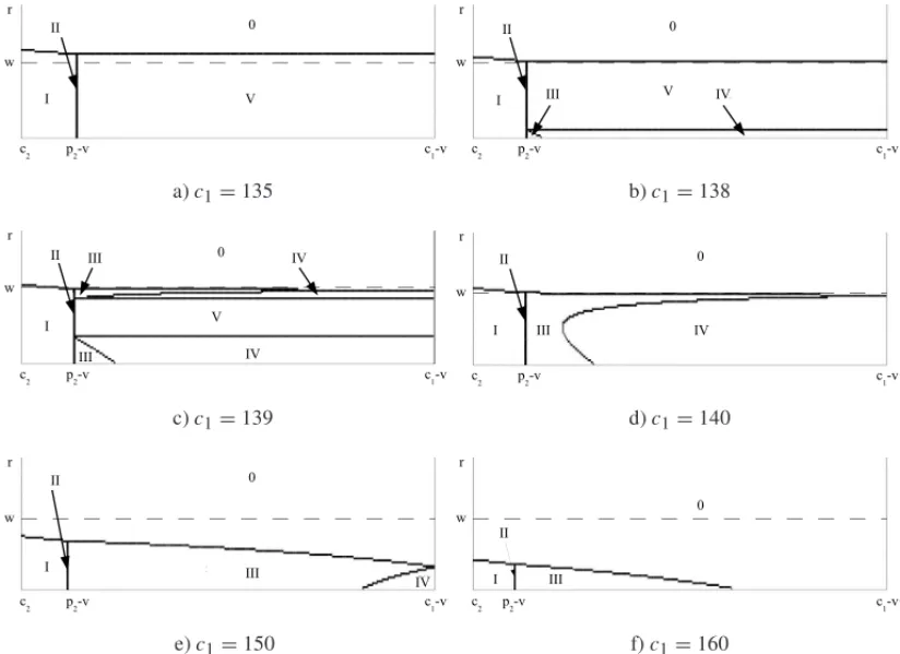
As shown through the analytical results, the return rater, and the repair costc4are two of the main drivers of the optimal strategy. Hence, below we will provide numerical results as a function of these two problem characteristics. Figure 1 shows the overall optimal strategy as a function of repair costc4and consumer returnsrfor a level of warranty claimsw=0.2 and different values of new production costc1.
First of all, we observe the trivial effect that with increasing costc1the OEM will accept less consumer returns from Figure 1. Further, the numerical results reconfirm that regardless of the consumer return rater and the new production costc1repair is the only option for dealing with warranty claims whenc4< p2−v(Scenario I).
More interestingly, forc4>p2−vthe figure nicely visualizes the change in the OEMs strategy asc1changes. Whenc1is rather small (Figure 1a), the production quantityq1and corresponding salesSD1(q1)are large enough to be able to deal with all warranty claims through replacement
and to use the remaining returns for serving the secondary market. Asc1increases, the resulting contraction of new productionq1induces the OEM to give up the secondary market whenr is small. Rather all the returns are used to replace as many warranty claims as possible (Scenarios III and IV in Figure 1b).
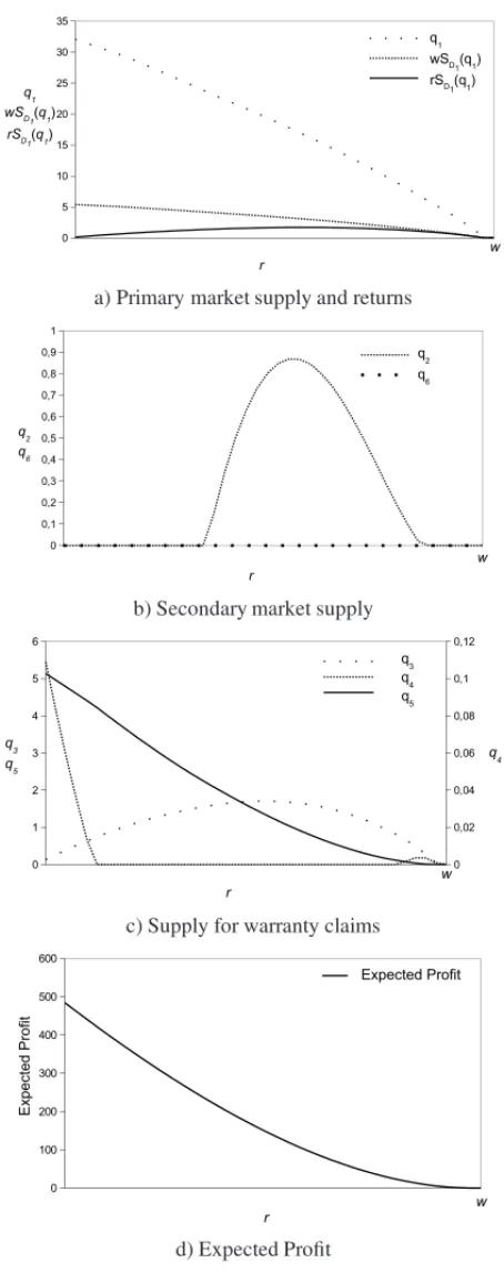
Asc1increases further, the OEMs strategy is characterized by the effect described when dis-cussing Proposition 3, see Figure 1c. Additionally, Figure 2 provides information about all the decision variables as a function ofrfor a level of repair costc4=65, which is slightly above the thresholdp2−v.
a)c1=135 b)c1=138
c)c1=139 d)c1=140
e)c1=150 f)c1=160
Figure 1– Optimal strategy as a function of repair costc4, rate of consumer returnsrand new production costc1(w=0.2,p1=183,p2=70,c2=50, v=10,D1∼U(0,100)).
ment as the sole warranty servicing strategy (Strategy V). These effects are nicely highlighted in Figures 2b and c.
While the effect concerning the secondary market has been discussed above in the context of Proposition 3, the optimal warranty servicing strategy deserves some focus here. When looking at Figure 2c we observe that for smallr repair and replacement form the optimal approach to-wards warranty claims. With increasingrrepair is reduced and eventually completely stopped. This behavior is induced by the increase in available consumer returns as shown in Figure 2a. Whileq1, and consequently the number of warranty claimswSD1(q1)continuously fall with
increasingr, the number of consumer returnsr SD1(q1)first increases and then falls. This latter
fall in the number of consumer returns also triggers another strategy switch, where the OEM eventually starts to use repair as part of its warranty servicing strategy again. In this case the amount of available returns is no longer sufficient to cover all warranty claims.
a) Primary market supply and returns
b) Secondary market supply
c) Supply for warranty claims
d) Expected Profit
Figure 2– Optimal production and supply quantities for primary market, secondary market and warranty claims as well as optimal expected profits as a function of rate of consumer returnsr (c4=65,p1=183,
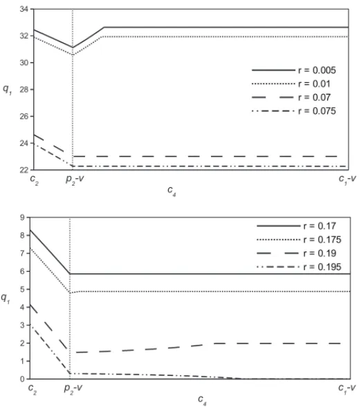
To conclude our results concerning the structural properties of the OEMs optimal strategy, let us revisit and visualize the result from Proposition 2. Figure 3 shows the optimal new production quantityq1as a function of repair costc4for different levels ofr.
Figure 3– Optimal level of new production as a function of rate of consumer returnsr and repair costc4 (p1=183,w=0.2,c1=139,p2=70,c2=50, v=10,D1∼U(0,100)).
Clearly, q1 falls asr increases as prescribed by Proposition 2 and also shown in Figure 2a. Concerning the relationship betweenq1 andc4 we see huge differences when comparing the various consumer return ratesr. From the left part of the figure we observe that for very small
In closing this section let us briefly comment on the performance implications of changes inr
andc4. It is quite clear that increases in the rate of consumer returns or the repair cost will always have detrimental effects on expected profits. This is exemplarily shown in Figure 2d.
4 CONCLUSION
In this paper we analyzed an OEMs optimal strategy for dealing with consumer returns under the requirement of servicing warranty. Using our model we characterized the different warranty servicing strategies, repair only, replacement only and the mixed approach. Further, we have shown under which conditions the OEM serves the secondary market. We find that the allocation of refurbished consumer returns is crucial but exhibits a non-trivial relationship between the secondary market and warranty servicing. Most interestingly and counter-intuitively our main findings show that when repair cost is within an intermediate range, the OEM may switch from a replacement only warranty servicing strategy to a mixed strategy including repair when the rate of consumer returns increases. As mentioned, this is due to a contraction in the new production quantity.
The link between warranty and consumer returns gives rise to a couple of interesting extensions of our model. One such extension deals with the OEMs optimal quality/durability choice for its new products. When increased R&D effort can help reducing warranty claims, while increased marketing (consumer information) effort can help reduce consumer returns, the question is how to optimally allocate the effort to these two strategies. Further, it is interesting to understand the conditions when either of the strategies is preferred.
Another important extension of the model concerns the temporal aspect related to consumer returns and warranty claims. As mentioned, consumer returns occur within up to 90 days after purchase, while warranties can extend over years. In [7] the necessity of fast reverse processes has been emphasized to account for the rapid reduction in value of returned, used products. In terms of our model this captures the trade-off between selling refurbished products on the secondary market and keeping them in stock for using them towards satisfying warranty claims at a later point in time. Besides inventory cost, the reduced value of such refurbished products will clearly influence the optimal strategy concerning the use of refurbished products towards warranty.
ACKNOWLEDGMENTS
This work has been supported by funds of the Oesterreichische Nationalbank (Anniversary Fund, project number: 14974). The authors gratefully acknowledge this financial support. The authors would like to thank Mike Galbreth and Gernot Lechner for valuable comments on the setup and framing of the model. Thanks also go to Gerald Senarclens de Grancy for help with the Figures.
APPENDIX
con-straint (6),i.e.at least oneλi =0,i ∈ {3,4,5}. Together with our assumptions p2−v >0 and
c4>0 this implies thatλw >0 in any feasible solution. Further,λrλ3λ5can’t be positive
accord-ing to the constraint (7) since the conditionsq3=0,q5=0 andq3+q5=q1−(1−r)SD1(q1)
can not hold at the same time. Note thatq1−(1−r)SD1(q1)is positive except forq1 = 0.
Finally, we are left with five scenarios in total satisfying these conditions and by combining the KKT conditions, we readily obtain Proposition 1.
Proof of Corollary 1. a) Plainly, in Scenario I repair is the only option for warranty claims. That is to say, if and only ifc4< p2−v, the OEM will choose repair as the exclusive option for dealing with defective units under the warranty scheme.
b) Obviously, the strategy of replacement only for warranty claims is possible in Scenarios II, III, IV and V. According to Scenario II, we obtainc4= p2−vandwSD1(q1)≤q1−(1−r)SD1(q1).
From Scenarios III and IV, we knowc4 > p2−v andw SD1(q1) = q1−(1−r)SD1(q1).
Finally, we havec4 > p2−v andw SD1(q1) < q1−(1−r)SD1(q1)based on Scenario V.
Hence, we learn that the OEM would like to replace all defective unites rather than repair them under the conditionsc4≥ p2−vandwSD1(q1)≤q1−(1−r)SD1(q1),i.e. c4≥ p2−vand r ≥w−q1−SD1(q1)
SD1(q1) .
c) Clearly, Scenarios II, III and IV are related to the situation that the secondary market is not served. For these three scenarios we respectively obtain the conditionsc4 = p2−v and wSD1(q1)≥q1−(1−r)SD1(q1), the conditionsc4>p2−vandwSD1(q1)≥q1−(1−r)SD1(q1)
and the conditionsc4>p2−vandwSD1(q1)=q1−(1−r)SD1(q1). In sum, we know whenever c4≥ p2−vandwSD1(q1)≥q1−(1−r)SD1(q1),i.e. c4≥ p2−vandr ≤w−
q1−SD1(q1)
SD1(q1) ,
hold, the OEM decides not to serve the secondary market.
Proof of Proposition 2. We can write[1−FD1(q1)]in Scenarios I, II, III, IV and V,
respec-tively as: c1−p2
(p1−p2) (1−r)−c2r−wc4,
c1−p2
(p1−p2) (1−r)−c2r−wc4,
c1−c4−v
(p1−p2) (1−r)−c2r−wc4−(1−r) (c4−p2+v),
c1−c4+λ4−v
(p1−p2) (1−r)−c2r−w (c4−λ4)−(1−r) (c4−λ4−p2+v),
c1−p2
(p1−p2) (1−r)−c2r−w (p2−v).
a) In Scenarios I, II and V, the coefficient ofris given by−(p1−p2)−c2<0. In Scenario III the coefficient ofris−(p1−p2)−c2+(c4−p2+v)= −p1−c2+c4+v <−p1−c2+c1<0. And in Scenario IV the coefficient ofris−(p1−p2)−c2+(c4−λ4−p2+v) <−p1−c2+c4−λ4+v= −p1−c2+λw+v <−p1−c2+c4+v <−p1−c2+c1<0. So denominators of 1−FD1(q1)
in all five scenarios decrease whenrincreases. It means that for all five scenarios 1−FD1(q1)
increases whenr increases. As a result, q1 is always decreasing when the rate of consumer returnsrincreases.
b) Similarly, it is clear to observe that in Scenarios I and IIq1decreases with increasing repair costc4and in Scenario Vq1is not affected by the repair costc4. Let us consider the derivative ofFD1(q1)with respect toc4for Scenarios III and IV. The derivative of FD1(q1)with respect to c4in Scenarios III and IV are
p1−c1−w (c1−v)+(c1−p1−c2)r
and
p1−c1−w (c1−v)+(c1−p1−c2)r
[(p1−p2) (1−r)−c2r−w (c4−λ4)−(1−r) (c4−λ4−p2+v)]2
respectively. Obviously, whenr < (p1−c1)−w (c1−v)
(p1−c1)+c2 , FD1(q1)is positive in Scenarios III and
IV. That is to say, in Scenarios III and IV q1increases with increasing repair costc4 ifr <
(p1−c1)−w (c1−v)
(p1−c1)+c2 and otherwise decreases. In sum,q1is non-decreasing wheneverc4> p2−v
andr < (p1−c1)−w (c1−v)
(p1−c1)+c2 , and is non-increasing with increasing repair costc4otherwise.
Proof of Proposition 3. When D1 ∼ U[0,b1], we know FD1(q1) =
q1
b1 and SD1(q1) =
q1− q2
1
2b1.
a) In Scenario V we haveλw =p2−vandλr =0. So we obtain
q1
b1
=(p1−p2) (1−r)−c2r−w (p2−v)−(c1−p2) (p1−p2) (1−r)−c2r−w (p2−v)
=(p1−p2)−w (p2−v)−(c1−p2)−(p1−p2+c2)r (p1−p2)−w (p2−v)−(p1−p2+c2)r
= NV −ZVr DV −ZVr .
Then we can rewritewSD1(q1) < q1−(1−r) SD1(q1)as(w+1−r)
2− NV−ZVr DV−ZVr
<2,
i.e. ZV r2− [2DV −NV −(1−w)ZV]r+w (2DV −NV)−NV <0. Hence, the existence
condition of Scenario V follows.
b) In Scenario III we haveλw =c4andλr =c4−(p2−v). So we obtain
q1
b1
= (p1−p2) (1−r)−c2r−wc4+r(c4−p2+v)−(c1−p2) (p1−p2) (1−r)−c2r−wc4−(1−r) (c4−p2+v)
= NI I I−ZI I Ir DI I I −ZI I Ir .
Then we can rewritewSD1(q1) >q1−(1−r)SD1(q1)as(w+1−r)
2− NI I I−ZI I Ir DI I I−ZI I Ir
>2,
i.e. ZI I I r2− [2DI I I −NI I I−(1−w)ZI I I]r+w (2DI I I −NI I I)−NI I I >0. Hence, the
existence condition of Scenario III follows.
REFERENCES
[1] AKCAY Y, BOYACIT & ZHANGD. 2013. Selling with money-back guarantees: The impact on prices, quantities, and retail profitability.Production & Operations Management, forthcoming. [2] BLACKBURNJD, GUIDEJRVDR, SOUZAGC & VANWASSENHOVELN. 2004. Reverse supply
[3] BLISCHKE WR & MURTHY DNP. 1992. Product warranty management – I: A taxonomy for warranty policies.European Journal of Operational Research,62: 127–148.
[4] DAVIS S, GERSTNER E & HAGERTY M. 1995. Money back guarantees in retailing: Matching products to consumer tastes.Journal of Retailing,71: 7–22.
[5] GEYERR, VANWASSENHOVELN & ATASUA. 2007. The economics of remanufacturing under limited component durability and finite product life cycles.Management Science,53: 88–100. [6] GUIDE JR VDR & VAN WASSENHOVELN. 2009. The evolution of closed-loop supply chain
research.Operations Research,57: 10–18.
[7] GUIDEJRVDR, SOUZAGC, VANWASSENHOVELN & BLACKBURNJD. 2006. Time value of commercial product returns.Management Science,52: 1200–1214.
[8] FERGUSONME, GUIDEVDR JR. & SOUZAGC. 2006. Supply chain coordination for false failure returns.Manufacturing & Service Operations Management,8: 376–393.
[9] FERGUSONME, FLEISCHMANNM & SOUZAGC. 2011. A profit-maximizing approach to disposi-tion decisions for product returns.Decision Sciences,42: 773–798.
[10] INDERFURTHK,DEKOKAG & FLAPPERSDP. 2001. Product recovery in stochastic remanufactur-ing systems with multiple reuse options.European Journal of Operational Research,133: 130–152. [11] ISKANDARBP, MURTHYDNP & JACKN. 2005. A new repair-replace strategy for items sold with
a two-dimensional warranty.Computers & Operations Research,32: 669–682.
[12] KHOUJAM. 1999. The single-period (news-vendor) problem: literature review and suggestions for future research.Omega,27: 537–553.
[13] LIX, LIY & CAIX. 2011. Quantity decisions in a supply chain with early returns remanufacturing.
International Journal of Production Research,50: 2161–2173.
[14] MURTHYDNP, DJAMALUDINI & WILSONRJ. 1995. A consumer incentive warranty policy and servicing strategy for products with uncertain quality.Quality and reliability engineering interna-tional,11: 155–163.
[15] MURTHYDNP & BLISCHKEWR. 1992. Product warranty management – III: A review of mathe-matical models.European Journal of Operational Research,63: 1–34.
[16] MURTHYDNP & DJAMALUDINI. 2002. New product warranty: A literature review.International Journal of Production Economics,79: 231–260.
[17] MURTHYDNP & NGUYENDG. 1988. An optimal repair cost limit policy for servicing warranty.
Mathematical and Computer Modelling,11: 595–599.
[18] NGUYENDG & MURTHY DNP. 1986. An optimal policy for servicing warranty.Journal of the Operational Research Society37: 1081–1088.
[19] NGUYENDG & MURTHYDNP. 1989. Optimal replace-repair strategy for servicing items sold with warranty.European Journal of Operational Research,39: 206–212.
[21] SHULMANJD, COUGHLANAT & SAVASKANRC. 2009. Optimal restocking fees and information provision in an integrated demand-supply model of product returns.Manufacturing & Service Oper-ations Management,11: 577–594.
[22] SHULMANJD, COUGHLANAT & SAVASKANRC. 2011. Managing consumer returns in a compet-itive environment.Management Science,57: 347–362.
[23] SOUZA GC. 2013. Closed-loop supply chains: A critical review, and future research. Decision Sciences, forthcoming.
[24] YALABIK B, PETRUZZI NC & CHHAJED D. 2005. An integrated product returns model with logistics and marketing coordination.European Journal of Operational Research,161: 162–182. [25] ZUO MJ, LIUB & MURTHY DNP. 2000. Replacement-repair policy for multi-state deteriorating