Forecasting stock-return volatility in the time-frequency domain

Forecasting Stock-Return

Volatility in the time-frequency

domain

Final Dissertation Work presented to Universidade Católica Portuguesa

to obtain the degree of Master Degree in Finance

by

Gui Duarte Diniz de Abreu Bragança Retto

(PhD) Prof. Gonçalo Faria and (PhD) Prof. Fábio Verona

iii

Acknowledgments

First and foremost, I would like to express my profound gratitude to both Prof. Gonçalo Faria and Prof. Fabio Verona for their valuable guidance, for all the support they gave this research and for always steering me into the right direction. Definitively, they were always available to answer my questions, providing me the answers, tools and feedback that allowed me to successfully complete my dissertation.

I would also like to thank my family for providing me unfailing supporting as well as continuous encouragement throughout all my years of study that culminated with writing this thesis. This accomplishment would not have been possible without them.

Finally, I would like to dedicate this dissertation to my grandmother, Marisa, who recently passed away. I will never forget you.

v

Resumo

Este estudo foca nos modelos autorregressivos de heterocedasticidade condicional, em especial nos modelos GARCH. A amostra principal usa dados do retorno do índice do S&P500 ajustados a divisão e dividendos de 1990 a 2008, usando uma janela fora da amostra de 2001 até ao final da amostra. O objetivo principal é analisar o desempenho das previsões do modelo num domínio tempo-frequência e, em seguida, compará-los com resultados em um cenário de domínio de tempo. Para fazer uma análise de domínio tempo-frequência, usamos técnicas de wavelets para decompor as séries temporais S&P500 originais em diferentes frequências, cada uma delas originalmente configurada no domínio do tempo. Em última análise, o objetivo é ver se a decomposição com wavelets traz um desempenho aprimorado na previsão/modelagem da volatilidade, observando a função de perdas de previsão de Quasi-Verossimilhança (QL), bem como os índices médios de perdas de previsão ao quadrado (MSFE). Embora a decomposição com wavelets ajude a capturar componentes periódicos ocultos das séries temporais originais, os resultados de domínio de frequência em termos de função de perda (QL e MSFE) não superam o resultado original do domínio do tempo para qualquer frequência dada. No entanto, a maioria das informações para a volatilidade futura é capturada em poucas frequências da série temporal do S&P500, especialmente, na parte de alta frequência dos espectros, representando horizontes de investimento muito curtos.

Palavras-chave: volatilidade, GARCH, decomposição com wavelets, função de perdas

vii

Abstract

This research focuses on generalized autoregressive conditional heteroskedasticity (GARCH) model. The main sample uses daily split-adjusted and dividend-split-adjusted log-return data of the S&P500 index ranging from 1990 to 2008, using an out-of-sample window from 2001 until the end of the sample. The main goal is to analyze the performance of the model forecasts in a time-frequency domain and then to compare them with results in a time-domain scenario. To make a time-frequency domain analysis, this research uses wavelets techniques to decompose the original S&P500 time series into different frequencies brands, each of them originally set in time-domain. Ultimately, the aim is to see if the wavelet decomposition brings an enhanced performance on forecasting/modelling volatility by looking at the Quasi-Likelihood forecasting losses (QL) as well as the mean squared forecasting losses ratios (MSFE). Although the wavelet decomposition helps to capture hidden periodic components of the original time-series, frequency-domain results in terms of loss function (QL e MSFE) don’t outperform the original time-domain result for any given frequency. Nevertheless, most of the information for future volatility is captured in few frequencies of the S&P500 time-series, specially in the high-frequency part of the spectra, representing very short investment horizons.

ix

Content

List of Tables ... xiii

1- Introduction ... 1

2- Literature Review ... 5

2.1- Modelling and Forecasting Volatility ... 5

2.2- Forecasting Stock-Return Volatility ... 8

2.3- Forecasting in Frequency-Domain ... 13

2.4- Frequency Decomposition ... 15

2.4.1- Wavelets ... 15

3-Data ... 19

4-Methodology and Forecasting Evaluation ... 20

4.1- Forecasting Procedure ... 20

4.2- GARCH ... 21

4.3- Volatility Proxy ... 23

4.4- Loss Functions and MSFE ratios ... 24

5-Frequency-Domain Methodology ... 27

5.1- Wavelets ... 27

5.2- Forecasting evaluation in the frequency-domain ... 30

6- Results ... 31

7- Conclusions ... 33

8- Bibliography ... 34

xi

List of Figures

Figure 1- Full Sample Returns and Inferred Volatility ... 40

Figure 2- Autocorrelation function of S&P500 returns and squared returns ... 41

Figure 3-Autocorrelation function of standardized residuals and squared standardized residuals 42 Figure 4- S&P500 returns in the OOS period ... 43

Figure 5- OOS ex-post proxy (r2) values ... 44

Figure 6- OOS GARCH (1,1) volatility forecasts ... 45

Figure 7- Daily OOS QL loss values ... 46

Figure 8- OOS S&P500 decomposed returns in 𝐷2 frequency (short-term) ... 47

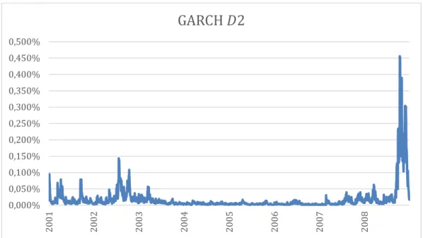
Figure 9- OOS GARCH (1,1) volatility forecasts based on S&P500 𝐷2 frequency ... 48

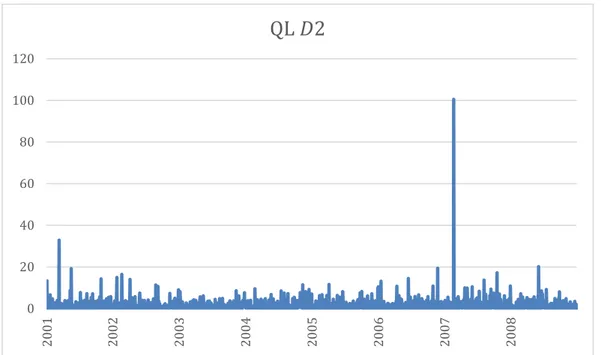
Figure 10- OOS QL loss values in D2 frequency ... 49

xiii

List of Tables

Table 1- GARCH (1,1) full sample parameter estimation ... 51

Table 2- Full sample variables summarized statistics ... 52

Table 3- Mean QL loss, MSFE PM, MSFE GARCH and MSE ratio in OOS period ... 53

1- Introduction

Stock market volatility is a statistical measure of the dispersion of returns for a given security or market index. It is measured by using the standard deviation of logarithmic returns or variance between returns over a given period. Usually, the higher the volatility, the higher the potential returns, but they come with greater risk. Stock market volatility is thus a market measure for economic uncertainty.

It’s important to understand the dynamics of stock market volatility since it’s a topic of major interest to policy makers and market practitioners. In particular, policy makers are interest in the determinants of volatility and its effects on economy, while market practitioners are interested in analyzing the effects of volatility on the pricing and hedging of derivatives position, since the price of every derivative security is affected by volatility fluctuations. In both cases, forecasting stock market volatility constitutes a fundamental instrument to risk management where Value-at-Risk models are the most commonly used. Even portfolio management models, such as the CAPM (Sharpe, 1964), are based on the “mean variance” theory, and therefore considers volatility as a key factor.

A problem about volatility is that it isn’t directly observed (like returns are), and thus needs to be estimated. In fact, we can see this from the Black and Scholes (1973) formula, in which volatility is the only unknown parameter/variable and needs to be forecasted. It has been pointed out that option prices (reflected in implied volatility) should have information about future market stock return. At that point in time (1980’s), forecasting volatility was easier since almost all options traded had short maturity dates, and for that reason volatility was assumed to remain almost constant. However, the

2

derivative market has since then grown exponentially and we can now find an enormous number and contracts with different and longer maturity periods, making it difficult to accurately price the value of such products, since volatility changes over long periods of time. For this reason, proxies are generally constructed and used to measure and model volatility. One popular approach is to use the daily squared returns (r2) as an ex-post proxy, which this study considers to evaluate volatility forecasts accuracy. Although it’s considered to be a noisy proxy, it does capture one of volatility key features that is, that volatility isn’t constant and varies over time. Another related property, is that conditional variance exhibits momentum, and for that reason past volatility can be used to explain current volatility (de Pooter, 2007).

The most widely used model to illustrate and capture the conditional variance is the generalized autoregressive conditional heteroskedasticity (GARCH) model proposed by Engle (1982), Bollerslev (1986) and Taylor (1986).

This study explores the performance of stock return volatility forecasting within the class of autoregressive conditional heteroskedasticity models, especially focusing on the GARCH (1,1) model since it’s considered to be the state-of-art model in the literature for this purpose. This model is usually preferred as it’s a better fit for modeling time series which data exhibits heteroskedasticity, volatility clustering, fat-tails distribution and price spikes.

While most of the literature on modeling and forecasting volatility has been only focused in time-domain analyses, this study uses a recent approach that focuses in a jointly time-frequency scenario. Particularly, wavelets techniques have recently provided great relevance in economic research these past years. These techniques are used to deeper analyze volatility’s behavior, which information is used with a forecasting purpose.

3

The aim of this study is to see if we can provide better insight and statistically significant improvements on forecasting and modeling volatility by using wavelets to decompose our original time series (in this case, the S&P500 return index) into different frequencies.

The remainder of this thesis is organized as follows: Section 2 gives a generalized literature review of the standard models used to forecast stock return volatility an extends this analysis into the frequency-domain, Section 3 discusses the data used, Section 4 explains the econometric framework used for forecasting volatility, the ex-post volatility proxy used to evaluate those forecasts and the frequency decomposition process as well as their evaluation. Section 5 reports the results of this research in both time and frequency domain. Finally, Section 6 concludes.

5

2- Literature Review

2.1- Modelling and Forecasting Volatility

Volatility modeling and forecasting has always been of interest for many financial analysis, options and portfolio management since it’s an important parameter for pricing financial derivatives. For obvious reasons, it’s not only important to know the current value of volatility, but also to evaluate how this value will evolve and what its future value is going to be. Forecasting volatility has been a much-debated topic over the years, since it’s a challenging and complex task to get an accurate prediction of its future values. While large positions in volatile assets are undesirable, since volatility reverts to a fixed mean and has zero expected return on the long-run, small positions can provide valuable hedging, for example, against crisis, lowering prices that drive simultaneously both correlations and volatilities up.

The main models to forecast volatility are time-series models and implied volatilities models, which rely on observed option prices.

Theoretically, the implied volatility from option prices should contain all relevant and available information and thus should be a good estimate of future realized volatility. However, this isn’t always the case, since there’s a risk premium because volatility risk cannot be perfectly hedged [as stated by Bollerslev and Zhou (2005)]. Another implication is that implied volatility is only available for certain time horizons and limited set of assets. Because of this, the most common used models for volatility forecasting are time series models, which are the models used in this research, focusing on the class of autoregressive conditional heteroskedastic models.

6

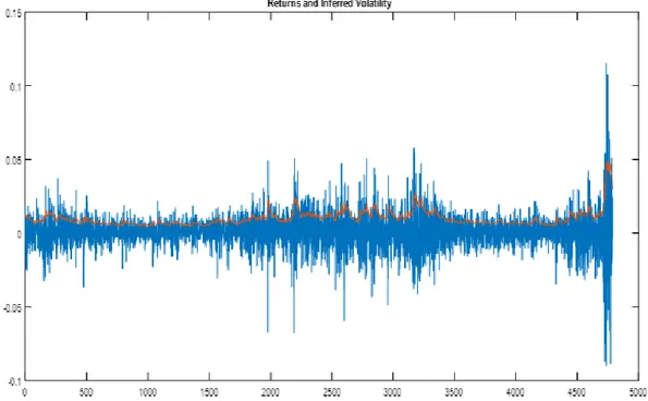
In almost all financial time-series the variance isn’t constant and changes over time, so models are heteroscedastic and time-series exhibit long-memory as well as volatility clustering, portraying periods of low market uncertainty followed by periods of high market uncertainty (or vice-versa). For example, volatility of S&P500 was extremely low during the years of 2003 to 2007, before reaching record-breaking values during the market collision of 2008 (see Figure A returns and inferred volatility over 4500 days and Figure F for the out-of-sample GARCH (1,1) volatility forecasts in the fall of 2008).

Modelling and forecasting volatility has been one of literature’s main challenge as it is complicated task to accurately estimate their future values. This research relates to the first main stream of literature that focuses on standard models used to make volatility forecasts.

Modeling and forecasting of volatility started when Engle (1982) developed the Autoregressive Conditional Heteroskedasticity (ARCH) model. The ARCH model, although it was first designed to measure and explain the dynamics of inflation uncertainty, was the earliest path-breaking model to explain non-linear dynamics and to model the conditional heteroscedasticity in volatility. It’s conditional because next period volatility (t+1) is conditional on the information set available at the current period (t), and heteroskedasticity means that volatility changes over time. One important feature of these models is that they assume that the conditional variance is a function of the squares of past observations as well as past variances, where the error term captures the residual result that’s left unexplained by the model. It also assumes that the variance of the current error term is related to the size of the previous year’s error terms. The ARCH models attempt to model the variance of those error terms and, at the same time, they try to correct the problems resulting from heteroskedasticity.

7

The Generalized Autoregressive Conditional Heteroskedasticity (GARCH) model is an extension of the ARCH model and was introduced by Engle (1982), Bollerslev (1986) and Taylor (1986). This is the state-of-art model for volatility forecasting [Zakaria and Shamsuddin (2012), Lindbald (2017)].

Similarly to ARCH models, GARCH models are used to model financial markets variables in which volatility varies over time, becoming more volatile in periods of financial distress and less volatile in periods of steady economic growth, hence exhibiting volatility clustering. 1 _{The model also uses values of} past squared observations as well as past variances to model the future variances at time t. Typically, the error term in traditional GARCH models is assumed to be normally distributed.

The ARCH and GARCH model have been extensively surveyed throughout the years [see e.g. Andersen and Bollerslev (1998), Bollerslev et al. (1994), Diebold (2004), Engle and Patton (2001)]. GARCH models are usually more preferred for forecasting applications because they describe volatility with less parameters, and, more importantly, they are less likely to breach the non-negativity constraint of the conditional variance (see sub-section 4.2).

Hansen and Lunde (2005) compared 330 different ARCH/GARCH models to test if any of those could outperform the standard GARCH (1,1) but they conclude that it can hardly be beaten.

GARCH models and their extensions are used to this day since they can account for characteristics that are commonly associated with financial time series (like excess kurtosis and volatility clustering).

The most commonly used approach for parameter estimation is by maximum likelihood (MLE), also, under the assumption that the standardized innovations (residuals) are i.i.d. normally distributed

8

In this study we use the GARCH (1,1) model. The first 1 in (1,1) refers to how many autoregressive lags (ARCH terms) appear in the equation, while the second 1 refers to how many moving average lags are used (GARCH terms)

2.2- Forecasting Stock-Return Volatility

This research is also related to another stream of literature that focuses on forecasting stock return volatility at different forecasting horizons. The volatility of stock returns captures the severity with which the market price of the security/stock fluctuates. The more swings it exists in prices, the more volatile the market is and thus the more unpredictable the future market stock price is going to be. When forecasting stock return volatility, the choice of how much data to use in estimation and forecasting as well as the forecasting horizon can be an issue if parameters are unstable, since data from distant past can bias estimates and thus produce inadequate forecasts.

The relationship between time-varying volatility and returns has been studied by Bollerslev et al. (1988), Bollerslev et al. (1992), Glosten et al. (1993), among others.

When forecasting and modelling stock return volatility, the focus has largely been on short-horizon forecast (usually one step-ahead forecasts) Engle (1982), Bollerslev (1986), Anderson and Bollerslev (1998), Brownless et al. (2011) and Lindbald (2017) show that, for those horizons, the GARCH (1,1) model performs well.

Even though longer horizons forecasts have been less emphasized, Ghysels et al (2006) showed that for longer horizons the GARCH-MIDAS model, an

9

extension of the GARCH model, generates better forecasts (forecasting advantages become more apparent at monthly horizons). Ghysels et al (2006) thus argue that, with GARCH extensions, volatility can be indeed forecastable at those horizons, making it a useful tool for risk management.

An extended theoretical overview of various key concepts of volatility modeling and forecasting is given by Poon and Granger (2003) and Anderson et al. (2006). Anderson et al. (2006) present a variety of procedures for volatility modeling and forecasting, based on GARCH, stochastic volatility models2

and realized volatility modelling. Anderson et al. (2006) extends this discussion to the multivariate problem of forecasting conditional covariance’s and correlations. They conclude by also giving insight into a topic of discussion of recent literature where they defend that the use of high frequency measures, data and predictors can significantly improve the volatility forecasting performance that will be discussed further.

Although GARCH models are considered to be the state-of-art for modelling and forecasting stock return volatility, they also have some flaws. First, both ARCH and GARCH models assume that positive and negative shocks on stock returns have the same impact in volatility. This, however, isn’t true and this asymmetry is considered to be one of the model’s biggest limitation. This asymmetry is generally known as the leverage effect: negative stock returns significantly increase volatility on the following days whereas positive stock returns don’t, or at least, not in the same proportion [Black (1976), Nelson (1991); Anderson et al. (2006); de Pooter (2007)]. A plausible explanation for this phenomenon is that the asymmetric relationship between

2 _{Stochastic volatility models are considered as complementary and not competitors of GARCH models since they}

10

the sign of stock returns and volatility is based on financial leverage. For example, a decrease in a stock value will increase financial leverage and, as a result, volatility goes up. For that reason, alternative GARCH formulations were first proposed by Black (1976). Additionally, literature has developed asymmetric models that could adjust for this phenomenon, like the Exponential GARCH (EGARCH) model proposed by Nelson (1991) which allows asymmetric effects of positive and negative shocks on returns.

Second, GARCH models tend to perform best under stable market conditions.

Moreover, as shown by Lindbald (2017) including macroeconomic variables seems to improve predictions of stock return volatility in recessions. Lindbald (2017) uses an asymmetric GJR-GARCH model proposed by Glosten et al. (1993), and also adjusts for leverage effect. Although there are periods where macroeconomic variables bring some predictability, Lindbald (2017) shows there are also periods where the GARCH (1,1) model produces more accurate forecasts.

Asymmetric models can be useful to adjust for this phenomenon, but empirical findings remain ambiguous since results aren’t clear cut. In fact, some authors defend that asymmetric GARCH models are unable to outperform the standard GARCH (1,1) (Van Dijk and Franses 1996) or their forecasting results don’t significantly improve compared to GARCH (1,1) forecasts (Ramasamy and Munisamy, 2012), while other authors argue that they can outperform them, especially in periods of recessions [Poon and Granger (2003); Brownlees et al. (2011)].

The difference in the empirical results mentioned above could be explained by different factors: the choice of the model, the length of the sample or frequency used, as well as the forecasting horizon.

11

Another typical limitation of GARCH models is that they often fail to fully capture the fat-tailed financial returns problem stated by Bollerslev (1986), even after adjusting for heteroskedasticity. This issue is also addressed in Brownlees et al. (2011) paper, they replace the simple Gaussian specification for a Student t likelihood function, but results aren’t as good as the proposed methodology, since it doesn’t bring statistically significant improvements. Connected to the fact that short horizon volatility doesn’t appear to violate the Gaussian assumption, while at longer horizons more tail events tend to exist, this research undertakes one-day ahead volatility forecasts.

In relation to the large literature on volatility forecasting of stock returns, Brownlees et al. (2011) explored their performance within the class of autoregressive conditional heteroskedasticity (ARCH) models and their extensions, demonstrating that the baseline GARCH model is a good descriptor of volatility, making it consistent with findings so far. Additionally, they evaluate volatility models across different forecasting horizons and asset classes.

Brownlees et al. (2011) use two ex-post proxies for S&P500 future volatility: the log squared returns (r2) and the realized volatility (RV) estimator from Anderson et al. (2003). 3 _{Both proxies are unbiased measures of true volatility.} Brownlees et al. (2011) results are reported by evaluating the model’s volatility forecasts using two loss functions, the quasi-likelihood (QL) and the mean squared error loss (MSE) functions. Even though better results are presented from the QL losses based on RV, Brownlees et al. (2011) defend that by using a sufficiently long out-of-sample history, results converge to similar values regardless of the proxy’s choice. Although data from distant past could bias

12

future estimates, this is a clear sign that models perform best when using longer data series. They also conclude there was no systematic large gains by modifying their base procedure with alternatives considered (by allowing for Student t innovations, short, medium or long estimation window).

The second part of 2008, known for being the start of the greatest crisis since the Great Depression of 1929, lead financial institutions to create a wide variety of “risk aversion” indicators. By computing the equity variance premium indicator 4 _{Bekaert and Hoerova (2014) showed it can be a} significant predictor of stock returns, while the conditional variance (which measures volatility and not stock returns) can’t, although the latter has a relatively higher predictive power for unstable financial conditions. The financial meltdown triggered in fact a near-record surge in volatility (VIX index, known as S&P500 “fear” index, hit highs of 80%), but surprisingly Brownlees et al. (2011) results based on one-day-ahead forecasts showed that there was no deterioration in the out-of-sample volatility forecasting accuracy during the turmoil, and although longer-horizons forecasts exhibit more deterioration and are larger in the tail of distribution, they argue that results from GARCH remained within a 99% confidence interval. Brownlees et al. (2011) also criticize one of the most widely used risk measures, the Value at Risk, since this measure focus on short-term risk although been used to measure the long-term risk.

In line with Brownlees et al. (2011) research, this study uses the daily squared returns (r2) as an ex-post proxy for future volatility, and evaluates the conditional variance forecasts by computing the Quasi-Likelihood loss

4 _{The difference between the squared VIX index and an estimate of the conditional variance of the stock}

13

function advocated by Patton (2009) and the mean square forecasting error ratio.

2.3- Forecasting in Frequency-Domain

The third stream of literature to which this research relates, is the one on modelling and forecasting financial and economic variables in a frequency-domain scenario.

Literature on forecasting stock market return volatility has mainly been focused on time-domain analysis, which is good for investors that tend to concentrate on stock market activity over the long horizons. A time-domain analysis aggregates the behavior of traders across all horizons, when in fact they make their decisions over different investment horizons as pointed out by Barunik and Vacha (2015), consistently with the Heterogeneous Market Hypothesis: the financial market is composed by participants that work over different trading frequencies

Recent developments on volatility forecasting include models based on high frequency volatility measures. As Anderson et al. (2003) point out, using volatility estimators to exploit the information contained in high-frequency data can bring substantially improvements, since such ex-post measures can be directly used for modelling and forecasting volatility dynamics. Engle and Gallo (2006), Corsi et al. (2010), Hansen et al. (2010), Mcmillan and Speight (2012) also made important contributions in this topic, suggesting that volatility can be directly observed when high frequencies data is applied.

Martens et al. (2004) propose a non-linear model for realized volatilities using high-frequency data that incorporates stylized facts of the GARCH volatility literature, particularly day-of-the-week effects, leverage effects and volatility level effects. They’re in-sample results show that all non-linearities

14

are highly significant and improve the description of the data. For shorter horizons up to 10 days, modelling these non-linearities produces superior volatility forecasts than a linear ARFI model, making it especially useful for short-term risk management. For longer time-horizons Martens et al. (2004) defend that incorporating these non-linearities don’t seem to bring benefits at all.

Note that the papers described above only look at data on different frequencies (for instance, using intra-daily data instead of daily-data) and not on frequency decomposition of an original time series.

Although there’s an extensive literature on modelling and forecasting volatility and some even do use high frequency measures, there’s yet to unveil the full potential of making a jointly time-frequency analysis.

In finance, the interest in frequency domain tools has been growing in recent years [e.g. Bandi et al. (2016); Barunik and Vacha (2017); Berger (2016) Faria and Verona (2018)], complementing a time-domain analysis by capturing hidden periodic oscillations and separating the noise of the short-term component from its trend (long short-term component). This research is related to these papers (and not to the previously papers that use high frequency data) since we use the same procedure, extracting the frequencies scales properly by pre-processing the original time-series with wavelet techniques. The main difference is that this research focuses on forecasting volatility at those exact scales that we get from frequency decomposition and not using a combination of different scales like Faria and Verona (2018). Therefore, the main research question is if frequency decomposition of the time-series can bring benefits in terms of modelling and forecasting stock return volatility. Ultimately, we evaluate the accuracy of results of the

15

estimation and compare them to the results from the original analysis (time-domain).

2.4- Frequency Decomposition

2.4.1- Wavelets

While most of the forecasting models are set in time-domain, wavelet transforms helps to make deeper analysis by extracting features from specific frequencies, representing the most recent milestone in financial econometrics. Since it’s a novel instrument it can be useful in many domains. By pre-processing data with wavelets, it allows to effectively account for hidden periodic components (Capobianco, 2004). Crowley (2007) and Aguiar-Conraria and Soares (2014) provided reviews of economic and finance applications of discrete and continuous wavelets tools.

Wavelet functions are useful tool for financial modeling and may be used for forecasting as well. Recent research have used wavelets with a forecasting purpose such as Rua (2011), Faria and Verona (2018), Barunik and Vacha (2017) and Berger (2016), and they already show great potential.

Through a wavelet multiresolution analysis, Rua (2011) decomposes time series into different time-scale components and fits a model to each scale. Rua (2011) proposes a wavelet approach for factor-augmented forecasting to test the forecasting ability of GDP growth, where results suggest that forecasting performance is enhance when factor-augmented models and wavelets are used together.

16

The discrete wavelet transform multiresolution analysis allows to decompose the original time series into its several components, each of them capturing the oscillations of the original variable within a specific frequency interval. Faria and Verona (2018) undertook this methodology, showing that the out-of-sample forecast of Equity Risk Premium (ERP) in the U.S. market can be significantly improved by considering the frequency-domain relationship between the ERP and several potential predictors.

In their working paper, Faria and Verona (2018) show that the low-frequency component (trend), of the term spread5 _{when properly extracted} from the data, is indeed a very strong equity risk premium out-of-sample predictor. It outperforms even the Short Interest Index (see Rapach et al. (2016), known for being the strongest predictor for ERP so far. Faria and Verona (2018) show that it has a remarkable forecasting power of ERP for different forecasting horizons both in-sample and out-of-sample periods, and that, there are significant utility gains when making forecasts using the proper frequency of the original time series.

When forecasting volatility in the frequency-domain, literature is very scarce and only started to be addressed in recent years, so it can be considered to be one of literature’s main gaps. However, first steps already have been taken by Barunik and Vacha (2015) and Berger (2016) that used wavelet tools with the purpose of studying volatility.

As traders operate over different time horizons6_{, Barunik and Vacha (2015)} use wavelets to decompose the integrated volatility into different time-scales, with high frequency data and multiple time-frequency decomposed volatility

5 _{Difference between the US long-term 10-year government bond and the 3-month Treasury bill} 6 _{The length of time that the investor expects to hold the security/portfolio}

17

measures. Their proposed methodology is moreover able to account the impact of jumps, using a jump wavelet two scale realized volatility estimator to measure exchange volatility in time-frequency domain and then study the influence of intra-day investment horizons on daily volatility forecasts. They compare their estimator to several most popular estimators (e.g. realized variance, bipower variance, among others) and Barunik and Vacha (2015) show that the wavelet based estimator proves to bring significant improvement in volatility estimation and forecasting.

A frequency decomposition of analysis of volatility parameters seems to be a useful tool for a forecasting purpose. It can also give interesting insights into the volatility process. More importantly, by undertaking a frequency-domain analysis, Barunik and Vacha revealed that “most of the information for future volatility comes from the high-frequency part of the spectra representing very short investment horizons” (Barunik and Vacha, 2015, p. 1).

To separate short-run noise from the long-run trends Berger (2016) used wavelet decomposition to transform financial return series into its frequencies and investigated the relevance of different timescales in the VaR framework, showing that the relevant information needed to compute daily VaR is described by different time-scales of the original returns series. It also unveils, that VaR forecasts are mainly captured by the first scales or frequency brands, comprising the short-run information.

The analysis of the conditional volatility forecasts based on different timescales achieved through wavelets has not yet been investigated further. Similarly to Rua (2011), Faria and Verona (2018) and Barunik and Vacha (2017), this research uses wavelets to frequency-decompose the time series of S&P500 returns. The aim is to separate the noise of financial returns

short-18

term components from its long-run trend and then use the information extracted within specific frequencies to forecast volatility. Ultimately, the evaluation of those results will show if the wavelet methodology brings any benefits to our forecasting procedure.

19

3- Data

This study uses daily split-adjusted and dividend-adjusted log-return data on the S&P500 index from the Center for Research in Security Prices (CRSP) DataStream. The sample period ranges from 1990 to 2008, which comprises periods of expansions as well as recessions, including the beginning of the Great Financial crisis in late 2008. An out-of-sample exercise is more relevant to evaluate effective return predictability in real time. So, this research, the out-of-sample period starts at 2001 and goes until the end of 2008.

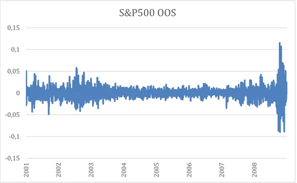
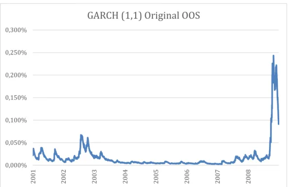
This out-of-sample period is characterized by episodes of high volatility (for example, the recessions from early 2000’s) as well as periods that exhibit low volatility levels (mostly, from 2003 to 2007). Furthermore, the data chosen also captures volatility forecasts during the triggering of the last great financial crisis at September 2008. In the fall of 2008, equity volatility in US reached a peak and volatility measures escalated in a matter of hours/days. We can see that from the last days (>4500 days) in Figure 1 that plots S&P500 returns which exhibit great dispersion during the turmoil and the inferred volatility at those days. We can see it more clearly in Figure 4 that plots the OOS S&P500 returns which took on a wider range of values than usual during the turmoil and in Figure 6 the OOS GARCH (1,1) volatility forecasts also increased in the fall of 2008.

20

4- Methodology and Forecasting Evaluation

4.1- Forecasting Procedure

Let {𝑦𝑡}𝑡𝑇 = 1 denote a time-series of continuously compounded returns

(including stock-splits and dividends) and 𝐼𝑡 denotes all historical known

information available at time 𝑡 . The unobserved variance of returns

conditional on the information available at t is therefore denoted as 𝜎_{𝑡+𝑖|𝑡}2 = var [𝑦_𝑡+𝑖|𝐼𝑡]. The variance predictions are obtained from volatility

models, which are generically represented as:

𝑦𝑡+1= 𝜖𝑡+1√𝑓𝑡+1 (3.1)

where 𝑓𝑡+1 is a measurable function due to the information available 𝐼𝑡 and

𝜖_𝑡+1 is an identically distributed zero mean and unit variance innovation. That is, the difference between the observed value of a variable at time t and the forecasted value based on information available prior to t, is assumed to follow a normal distribution. The parameter 𝑓𝑡+1 is determines the evolution

of the conditional variance, which is typically a function of historical returns as well as unknow parameters to be estimated. This is the parameter that volatility models try to predict.

The forecasting procedure is done as follows. For each day t of the sample, we estimate the model parameters by maximizing a Gaussian likelihood using all available returns and information ending prior to t. This research uses the GARCH (1,1) model to make one-day ahead forecasts, resulting in a daily volatility forecast path {𝑓𝑡+𝑖|𝑡}.

21

The out-of-sample forecasts are generated using a sequence of expanding windows. We use the initial sample until the end of the year 2000 to make the first OOS forecasts. Then, the sample is increased by one observation and thus a new OOS forecasts is produced. We make this procedure until the end of the full sample. The full OOS period therefore goes from January 2001 to December 2008.

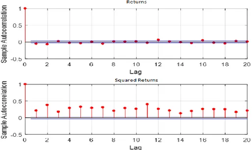
Before estimating our model and starting the forecasting procedure, we computed a sample autocorrelation function to see if S&P500 split-adjusted and dividend-adjusted returns exhibit serial correlation, this is, if past returns gives us any relevant information that would help to predict future returns. Looking the top graph at Figure 2, the answer is no since for all the lags they are barely statistically significant, underlying that past returns information isn’t useful and short-term returns are difficult to predict, which is a well-known fact.

4.2- GARCH

The GARCH (1,1) model from Engle (1982) and Bollerslev (1986) as said before, is seen in literature as the state-of-art model for forecasting volatility. It differs from a typical ARCH model by incorporating the squared conditional variance as an additional explanatory variable. The GARCH (1,1) describes the volatility process as:

The volatility process described by GARCH models is:

22

Where 𝜔 is the model’s constant, 𝛼 is the ARCH parameter and 𝛽 is the GARCH parameter. 𝑓𝑡+1 are the next period GARCH volatility forecast that’s

conditional on the combination of current squared returns (𝑟𝑡2) as well as

information available from current period forecasts.

The key features from this volatility process are its mean reversion (shown by the imposed restriction 𝛼 + 𝛽 < 1) and its symmetry, that is, the model considers that what influences future volatility is the magnitude of past returns, and not their signs. Another main restriction of the GARCH model is the non-linear constraint, that is, all the explanatory variables must be positive 𝜔 > 0; 𝛼 > 0; 𝛽 > 0); which can clearly be seen by the fact that it’s impossible to have a negative variance since it consists of squared variables. Note that the squared returns of our data are in the ARCH component.

GARCH model’s parameters coefficients are achieved by maximizing likelihood and their values are reported in Table 1. From the values t-statistics and comparing them with a normal distribution, we can clearly see that both ARCH and GARCH parameters reported in this table have a p-value< 0.01 so both parameters are statistically significant (null hypothesis rejected). Key variables calculated from our data are summarized in Table 2. Furthermore, Figure 1 plots the full sample conditional volatility forecasts (orange line, calculated from the squared root of conditional variance) as well as the original split-adjusted and dividend-adjusted S&P500 returns (blue line). Initially, the model seems to fit good to the data since it tracks well the volatility clusters, increasing the conditional volatility when they occur.

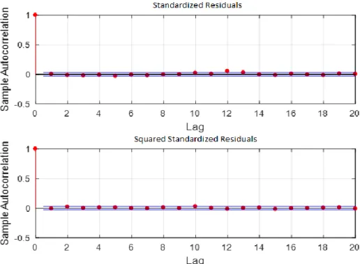
To check if it fits our data correctly, we also compute the standardized residuals (returns/conditional volatility) as well the squared standardized residuals and their sample autocorrelation function, where both should not exhibit serial correlation. From Figure 3, it seems that the standardized residuals and squared standardized residuals don’t exhibit serial correlation.

23

4.3- Volatility Proxy

Following most of the literature, this study uses daily squared returns 𝑟2 as an ex-post proxy for volatility, and can be obtained by squaring the split-adjusted and dividend-split-adjusted log returns of S&P500 index. So, for each day, we have an ex-post value for true volatility.

The variance of returns is denoted as follows:

𝜎𝑡2= 𝐸(𝑟𝑡2) − [𝐸(𝑟𝑡)]2 (3.3)

Which can be seen as the average of the squared returns differences from their mean. From the equation above (3.3), we can see why 𝑟2 is considered to be a noisy proxy for volatility, since we 𝜎𝑡2 ≅ E(rt2) under the strong

assumption that [𝐸(𝑟𝑡)]2 ≅ 0. Before high frequency data, many researchers

resorted to daily squared returns as a volatility proxy. Although being a noisy proxy, it’s an unbiased one and it reflects one of volatility key features: volatility isn’t constant and varies over time.

Moreover, and since squared returns are essentially representing our variance, we also computed a sample autocorrelation function. As we can see from the bottom graph in Figure 2, the squared returns do have serial correlation, statistically significant throughout the sample, meaning that past squared returns do capture information for future volatility.

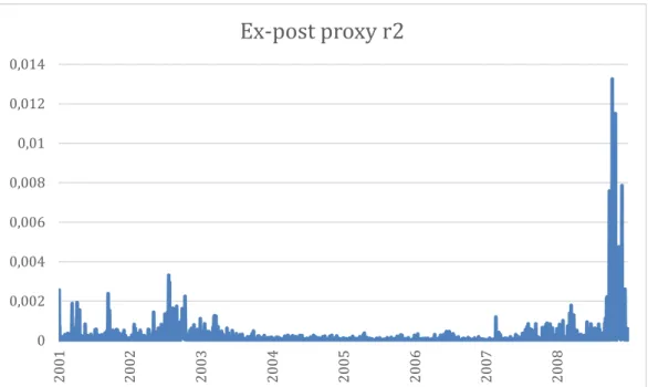
Since the proxy is used for an out-of-sample exercise, Figure 5 plots the squared returns values throughout the out-of-sample period. These values will be used to evaluate our model’s forecasting accuracy.

24

4.4- Loss Functions and MSFE ratios

To evaluate the accuracy of the results of the estimation this research uses the out-of-sample volatility forecast losses as suggested by Patton (2009). It’s a measure of predictive accuracy, so the smaller the average loss are, the better the model/proxy predictive power is. Table 3 summarizes the results and reports daily forecasting results for the GARCH model using the loss functions 𝐿(𝜎𝑡2, 𝑓𝑡|𝑡−𝑘). The main loss functions presented in this study is the

one that’s traditionally used in volatility forecasting literature: the quasi-likelihood (QL) loss function. Another way to evaluate the results is by analyzing our model’s MSFE ratios. This exercise is done in the out-of-sample period, since researchers consider to be a more effective measure to evaluate predictability. 𝑀𝑆𝐹𝐸𝑃𝑀 = 𝑚𝑒𝑎𝑛 [( 𝜎̂𝑡2)2− (𝐹𝐶𝑃𝑀)2] (3.4) 𝑀𝑆𝐹𝐸𝐺𝐴𝑅𝐶𝐻= 𝑚𝑒𝑎𝑛 [( 𝜎̂𝑡2)2− (𝑓𝑡|𝑡−𝑘) 2 ] (3.5) 𝑀𝑆𝐹𝐸 𝑟𝑎𝑡𝑖𝑜: 𝑀𝑆𝐹𝐸_{𝑀𝑆𝐹𝐸}𝐺𝐴𝑅𝐶𝐻 𝑃𝑀 (3.6) 𝑄𝐿: 𝜎̂𝑡2 𝑓_{𝑡|𝑡−𝑘}− log 𝜎̂_𝑡2 𝑓_{𝑡|𝑡−𝑘}− 1 (3.7)

Where 𝜎̂𝑡2 is an unbiased ex-post proxy of conditional variance [in this case

the squared returns (𝑟2)], and 𝑓𝑡|𝑡−𝑘 is volatility forecasts from the GARCH

25

mean squared forecasting error of our prevailing mean variance benchmark, mathematically, the mean of the difference of our squared proxy from our prevailing mean variance benchmark forecasts in the out-of-sample period. The same rational underlies the mean squared forecasting error of our GARCH model (𝑀𝑆𝐹𝐸𝐺𝐴𝑅𝐶𝐻), but this time, it is calculated instead from the

mean of the difference between our squared proxy and (𝑓𝑡|𝑡−𝑘) 2

, the latter being the our GARCH (1,1) squared volatility forecasts based on t-k information.

After computing the 𝑀𝑆𝐹𝐸𝑃𝑀 and 𝑀𝑆𝐹𝐸𝐺𝐴𝑅𝐶𝐻, we get the MFSE ratio by

dividing the mean squared error from the predictive model by the relative to the historical prevailing mean benchmark (𝑀𝑆𝐹𝐸_{𝑀𝑆𝐹𝐸}𝐺𝐴𝑅𝐶𝐻

𝑃𝑀 ).

Brownless et al. (2011) show that while the MSE loss depends on the additive forecast error (𝜎̂𝑡2− 𝑓𝑡|𝑡−𝑘)

2

, the QL loss depends on the

multiplicative forecast error 𝜎̂𝑡2

𝑓𝑡|𝑡−𝑘 . Brownlees et al. (2011) explains that since

QL loss function depends only on the multiplicative forecast error, the loss series is under the null hypothesis that the forecasting model (GARCH) is correctly specified. The mean-squared error, which depends on additive errors, scales with the square of variance and therefore can contain high levels of serial dependence even under the null.7 _{Brownlees et al. (2011) also states} that the bias of QL is independent of the volatility level while MSE has a bias proportional to the square of the true variance. This means that large MSE losses are a consequence of high volatility although not corresponding necessarily to a deterioration on the model’s forecasting ability. For these reasons, this research calculates the MSFE ratio relative to the prevailing mean instead of the MSE loss function.

7 _{If we divide MSE by 𝜎̂}

𝑡4 the resulting quantity will be independent and identically distributed under the null that the forecasting model is correctly specified.

26

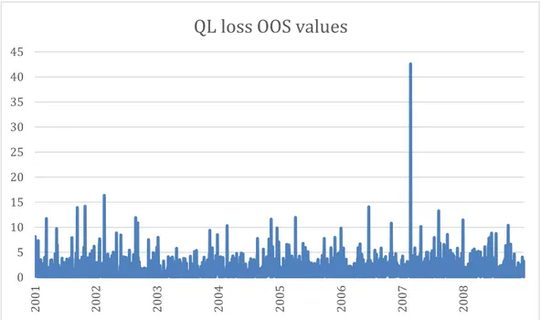
Figure 7 plots the out-of-sample QL loss values which this research uses to evaluate forecasting accuracy, while Table 3 reports the mean QL loss as well as the MSFE PM, the MSFE GARCH and the MSFE ratio relative to the prevailing mean in the OOS period.

27

5- Frequency-Domain Methodology

5.1- Wavelets

We now move to the analysis in the frequency-domain by decomposing the original time-series into several different components, each of them accounting for properties in that particular frequency brand and defined in time-domain.

To extract the frequencies from the S&P500, we use wavelets filtering methods. In line with Rua (2011) and Faria and Verona (2018), the frequency decomposition method used is known as maximal overlap discrete wavelets transform multiresolution analysis (MODWT MRA). Doing this will help re-evaluating the squared returns proxy as well the GARCH (1,1) forecasting performance by using information of each frequency components time series. By applying this method, the original time series of S&P500 index is decomposed into:

𝑆&𝑃500(𝑇𝑆,𝑡) = 𝑆&𝑃500(𝐷1)𝑡+. . . +𝑆&𝑃500(𝐷𝑗)_𝑡 + 𝑆&𝑃500(𝑆𝑗)_𝑡 (3.9)

Where 𝑆&𝑃500(𝑇𝑆,𝑡) is our original time-series of S&P500 index returns

throughout the full sample, &𝑃500(𝐷𝑗)_𝑡 , j = 1, 2,…, J are the wavelet details

or number of multiresolution scales under analysis and 𝑆&𝑃500(𝑆𝑗)𝑡 is the

wavelet smooth (low-frequency part of the spectra). The original time series of the S&P500 index is therefore decomposed into J+1 components [𝑆&𝑃500(𝐷₁)_𝑡 to 𝑆&𝑃500(𝐷𝑗)_𝑡 and 𝑆&𝑃500(𝑆𝑗)_𝑡 ] each defined in the

time-domain and representing the fluctuation of the original time series of S&P500 in a specific daily-frequency brand. For small j, the J wavelet components represent the higher frequency components of the original time-series, its

28

short-term dynamics. As J increases, the J wavelet components start representing lower frequencies movements of the original time-series, representing the long-term dynamics of our original variable. At last, the wavelets smooth captures the lowest frequency dynamics and so the original time-series trend. In other words, the discrete wavelet multiresolution analysis maps the original of S&P500 original time series in the time-domain and represents its constituents in a timescale domain.

Note that if all J+1 frequency-decomposed components are added, then the original time-series of S&P500 returns is recovered.

Considering the choice of J, the number of observations dictates the maximum number of frequencies that can be used. 8

This research performs a J=10 level MODWT MRA to the S&P500 time series using the Haar wavelet filter with reflecting boundary conditions9_. Since this research uses daily data, the first components 𝑆&𝑃500(𝐷1)𝑡

captures oscillations of the S&P500 time series between 2 and 4 days.

𝑆&𝑃500(𝐷2)𝑡 ; 𝑆&𝑃500(𝐷3)𝑡 ; 𝑆&𝑃500(𝐷4)𝑡 ; 𝑆&𝑃500(𝐷5)𝑡 ; 𝑆&𝑃500(𝐷6)𝑡 ;

𝑆&𝑃500(𝐷₇)_𝑡 ; 𝑆&𝑃500(𝐷8)𝑡 ; 𝑆&𝑃500(𝐷9)𝑡 and 𝑆&𝑃500(𝐷10)𝑡 capture

oscillations of the S&P500 returns between 4-8, 8-16, 16-32, 32-64, 64-128, 128-256, 256-512, 512-1024 and 1024-2018 days respectively. At last, the smooth component, 𝑆&𝑃500(𝑆𝑗)_𝑡, which can be re-denoted in 𝑆&𝑃500(𝐷11)𝑡 captures

the trend and oscillations of the S&P500 and volatility forecast with a period longer than 2018 days (see Figure 11)

8 _{Consider N as the number of observations in the IS period, J must satisfy the next constraint: 𝑁 > 2}𝐽_{. In} this research there’s 2779 IS observations.

29

By decomposing the original S&P500 into J+1 frequency we get new squared returns within each specific frequency for each day. Because of this, our volatility model will make forecasts using the information set available at those exact same frequencies as well as our newly squared returns for each specific scale. The main difference from our original 𝑓𝑡+1 volatility forecasts of

GARCH (1,1) model in (3.2) is that 𝑟𝑡2 is now a frequency decomposed

variable, so within each day we will have squared returns for all the different frequency used.

By doing so, it allows to evaluate the model’s conditional variance forecasts within a specific frequency and we’ll continue to make a daily OOS evaluation.

So, for each day of the sample we estimate:

𝑓𝑡+1|𝐷_𝐽 = 𝜔 + 𝛼𝑟𝑡|𝐷𝐽

2 _{+ 𝛽𝑓}

𝑡 (3.10)

By using these frequencies components, our volatility forecasts will be 𝑓_{𝑡+1|𝐷𝑗} for each day using a specific frequency of the S&P500 time-series.

So, for each OOS day we will have 𝑓𝑡+1|𝐷1; 𝑓𝑡+1|𝐷2; 𝑓𝑡+1|𝐷3; 𝑓𝑡+1|𝐷4; 𝑓𝑡+1|𝐷5; 𝑓_𝑡+1|𝐷6; 𝑓𝑡+1|𝐷7; 𝑓𝑡+1|𝐷8; 𝑓𝑡+1|𝐷9; 𝑓𝑡+1|𝐷10 and 𝑓𝑡+1|𝑆𝐽 where all first ten volatility forecasts are the ones based on S&P500 𝐷𝐽 corresponding frequency

component and 𝑓𝑡+1|𝑆𝐽 is the volatility forecasts based on the trend component of S&P500. We note that, the sum of all those frequency-decomposed variances forecasts within a day won’t give the original out-of-sample volatility forecasts from our GARCH model for that day.

30

5.2- Forecasting evaluation in the frequency-domain

To evaluate the forecasting ability of our GARCH (1,1) model, we continue to use the out-of-sample loss functions as well as the MSFE ratios explained in sub-section (4.4). Now, both functions are calculated using the frequency decomposed volatility forecasts.

The daily squared returns (r2) continues to be our ex-post proxy for volatility to make comparisons with the results we get from a time-frequency domain perspective. For example, the mean out-of-sample QL for oscillations between 4 and 8 days is calculated as:

QL|D2: mean( ∑ 𝜎 ̂_𝑡2 𝑓_𝑡+1|𝐷2 2011 𝑡=1 − log 𝜎 ̂_𝑡2 𝑓_𝑡+1|𝐷2− 1) (3.11)

Where 𝜎̂𝑡2 is the proxy values for volatility covering the OOS period

(2001-2008) and 𝑓𝑡+1|𝐷1 are GARCH (1,1) volatility forecasts for each out-of-sample day, based on the wavelet details being used (in this case, the out-of-sample volatility forecasts underlying the information between 4 and 8 days (𝐷2) of

S&P500 frequency decomposed time-series). The daily QL|D₂ losses are plotted

in Figure 10.

The same process is done for the MSFE ratios, that is, the 𝑀𝑆𝐹𝐸𝐺𝐴𝑅𝐶𝐻 now

31

6- Results

We now evaluate the variance forecasts of the GARCH (1,1) model by analyzing the daily out-of-sample QL loss function (see Figure 7) and MSFE ratios. Table 3 reports the results of the mean of QL losses and MSFE ratios throughout the out-of-sample (2001-2008) period. Those results are based only in a time-domain scenario. The mean QL loss of the GARCH (1,1) is quite high, which can be explained from the fact that our ex-post proxy captures much of the noise and the latter damages the forecasting accuracy. Interestingly, results from MSFE ratio are however significantly better. Recall that a MSFE ratio under 1 implies that the model produces more accurate volatility forecasts than the historical prevailing mean variance benchmark.

After making a time-domain analysis, we extend this research by addressing estimations of volatility forecast in a frequency decomposed scenario and their respective evaluation. The aim is to see if by de-noising and capturing hidden periodic components of the original S&P500 time series, brings benefits compared to Brownlees et al. (2011) original forecasts evaluation. To evaluate the predictability of a frequency decomposed method, we compute both QL losses and MSFE ratios for each specific frequency being used. Summarized frequency-decomposed results are reported in Table 4. Overall, the best frequency-decomposed result was given with wavelet filter haar (also known as db1) using a frequency scale of 4-8 days.10 _{This is}

consistent with Barunik an Vacha (2015) and Berger (2016) findings that most of the information for future volatility comes from the high-frequency part of

10 _{This research also considered different type of filtering methods like Daubechies (from d2 to d12) Symlets (from}

sym2 to sym12) and Coiflets (coif 2, coif4, coif5) although none of these presented better results than the reported Haar filter

32

the spectra representing very short investment horizons, since the frequency 𝐷2 represents S&P500 index short term dynamics. Frequencies from 8-16 until

512-1024 days ( 𝐷3 to 𝐷9 ), were the frequencies that exhibited most

deterioration in terms of QL losses and MSE ratios, especially the frequency 32-64 (𝐷5) that reached mean high QL losses of 45,31) making it clear that all

those frequencies aren’t desirable to use for a forecasting purpose. The last frequency 𝐷11 is plotted in Figure 11 and captures the trend of S&P500

original series.

It’s clear that for all the frequencies used both QL losses and MSFE ratios are higher than the original time-domain analysis.

33

7- Conclusions

Although wavelet techniques are indeed a useful tool and can be successfully used to forecast economic and financial variables summarized results from this study demonstrate that there’s no increases in the predictability of volatility. We evaluate this predictability by computing both QL losses and MSFE ratios for the different frequencies used, and we see that for all the frequencies, both of QL losses and MSFE ratios results are higher than the original analysis. Hence, the frequency-domain results aren’t better than those achieved in a time-domain scenario. Despite this fact, they show that volatility forecasting losses are smaller when high frequencies are used. In fact, the 4 to 8 days frequency gives the best results since it has the lowest QL loss and MSFE ratio from all the frequency brands (see Figure 8, Figure 9 and Figure 10).

This research is a first step towards a better understanding of decomposed univariate financial time-series. It remains to be tested in future research different frequencies combinations and their respective forecasts, since this research only focus on each specific frequency brand. It would also be interesting to undertake the same methodology using high frequency measures to proxy for future volatility, since many authors defend they exhibit some potential.

34

8- Bibliography

Aguiar-Conraria, L. and Soares M. J. (2014). The Continuous Wavelet Transform: Moving Beyond Uni and Bivariate Analysis. Journal of Economic Surveys 28(2), 344-375.

Andersen, T. G. and Bollerslev, T. (1998). Answering the skeptics: Yes, standard volatility models do provide accurate forecasts. International Economic Review, 39(4), 885-905.

Andersen, T. G., Bollerslev, T., Christoffersen, P. F., and Diebold, F. X. (2006). Volatility and correlation forecasting. Handbook of economic forecasting, 1, 777-878.

Andersen, T., Bollerslev, T., Diebold, F., and Labys, P. (2003). Modeling and forecasting realized volatility. Econometrica, 71(2), 579-625.

Bandi, F., Perron, B., Tamoni, A. and Tebaldi, C. (2016). The Scale of Predictability, Working Papers 509

Barunik, J. and Vacha, L. (2015). Realized wavelet-based estimation of integrated variance and jumps in the presence of noise. Quantitative Finance 15(8), 1347-1364.

Bekaert, G., and Hoerova, M. (2014). The VIX, the variance premium and stock market volatility. Journal of Econometrics, 183(2), 181-192.

35

Berger, T. (2016). Forecasting Based on Decomposed Financial Return Series: A wavelet analysis. Journal of Forecasting, 35, 419-433.

Black, F. (1976). Studies of stock market volatility changes. Proceedings of the American Statistical Association, Business and Economic Statistics Section, 177– 181.

Black, F. and Scholes, M. (1973). The pricing of options and corporate liabilities. Journal of political economy, 81(3), 637-654.

Bollerslev, T. (1986). Generalized Conditional Autoregressive Heteroscedasticity. Journal of Econometrics, 31, 307-327.

Bollerslev, T., Chou, R. and Kroner, K. (1992). ARCH modeling in finance: A selective review of the theory and empirical evidence. Journal of Econometrics 52, 5–59.

Bollerslev, T., Engle, R.F. and Nelson, D.B. (1994). ARCH models. Handbook of Econometrics, 4. 2959–3038.

Bollerslev, T., Engle, R.F. and Wooldridge, J.M. (1988). A capital asset pricing model with time varying covariances. Journal of Political Economy 96, 116–131.

Bollerslev, T. and Zhou, H. (2005). Volatility puzzles: A simple framework for gauging return-volatility regressions. Journal of Econometrics 131, 123-150.

36

Brownlees, C. and Gallo, G. (2006). “Financial econometric analysis at ultra highfrequency: data handling concerns”. Computational Statistics and Data Analysis 51(4), 2232–2245.

Brownlees, C., Engle, R. and Kelly, B. (2011). A practical guide to volatility forecasting trough calm and storm. Journal of Risk, 14(2), 3-22

Brownlees, C., Engle, R. and Kelly, B. (2011). A practical guide to volatility forecasting through calm and storm (Appendix). Technical Report.

Capobianco, E. (2004). “Multiscale Analysis of Stock Index Return”. Computational Economics 23, 219–237.

Corsi F., Pirino, D. and Renò, R. (2010). Threshold Bipower Variation and the Impact of Jumps on Volatility Forecasting, Journal of Econometrics 159(2), 276-288.

Crowley, P. M. (2007). A Guide to Wavelets for Economists. Journal of Economic Surveys 21(2), 207-267.

de Pooter, M. (2007). Modelling and forecasting stock return volatility and the term structure of interest rates. (No. 414). Rozenberg Publishers.

Diebold, F.X. (2004). The Nobel memorial prize for Robert F. Engle. Scandinavian Journal of Economics 106, 165–185.

Engle, R. (1982). Autoregressive conditional heteroscedasticity with estimates of the variance of United Kingdom inflation. Econometrica 50(4), 987–1007.

37

Engle, R. and Gallo, G. (2006). A multiple indicators model for volatility using intradaily data. Journal of Econometrics 131(1), 3–27.

Engle, R. and Patton, A.J. (2001). “What good is a volatility model?”. Quantitative Finance, 1, 237–245.

Faria, G. and Verona, F. (2018). The equity risk premium and the low frequency of the term spread, Working Paper available at SSRN

Faria, G. and Verona, F. (2018). Forecasting stock market returns by summing the frequency decomposed parts. Journal of Empirical Finance, 45, 228-242.

Ghysels, E., Santa-Clara, P. and Valkanov, R. (2006). Predicting volatility: getting the most out of return data sampled at different frequencies. Journal of

Econometrics, 131(1-2), 59-95.

Glosten, L. R., Jagannathan, R. and Runkle, D. E. (1993). On the Relation Between the Expected Value and the Volatility of the Nominal Excess Return on Stocks, Journal of Finance, 48, 1779–1801.

Hansen, Peter R. and Lunde, A. (2005). A forecast comparison of volatility models: Does anything beat a garch (1,1)? Journal of Applied Econometrics 20, 873–889.

Lindbald, A. (2017). Exploring the time-variation in long-term stock market volatility forecasts, Unpublished paper, University of Helsinki.

38

Martens, M. and Zein, J. (2004). Predicting Financial Volatility: High-Frequency Time Series Forecasts Vis-`a-Vis Implied Volatility, Journal of Futures Markets, 24, 1005–1028.

Mcmillan, D. G. and Speight, A. E. H. (2012). Daily FX Volatility Forecasts: Can the GARCH (1,1) Model be beaten using high-frequency data?, Journal of Forecasting, 31(4) 330-343.

Nelson, D. B. (1991). Conditional Heteroskedasticity in asset returns: a new approach. Econometrica 59(2), 347-370.

Patton, A. (2009). Volatility forecast comparison using imperfect volatility proxies. Journal of Econometrics, 160, 246-256.

Poon, S. and Granger, C. J. (2003). Forecasting volatility in financial markets: a review. Journal of Economic Literature, 51(2), 478–539.

Poon, S. and Granger, C. (2005). Pratical issues in forecasting volatility. Financial analysts journal, 61(1), 45-56.

Ramasamy, R. and Munisamy, S. (2012). Predictive accuracy of GARCH, GJR and EGARCH models select exchange rates application. Global Journal of Management and Business Research, 12(15).

Rapach, D. E., Ringgenberg, M. C., and Zhou, G. (2016). Short interest and aggregate stock returns, Journal of Financial Economics, 121(1), 46-65.

39

Rua, A. (2011). A wavelet approach for factor-augmented forecasting. Journal of Forecasting 30(7), 666-678.

Sharpe, W. F. (1964). Capital asset prices: A theory of market equilibrium under conditions of risk. The journal of finance, 19(3), 425-442.

Van Djick, D. and Franses, P. H. (1996). Forecasting stock market volatility using (non-linear) Garch models. Journal of Forecasting, 15(3), 229-235´

Zakaria, Z. and Shamsuddin, S. (2012). Empirical evidence on the relationship between stock market volatility and macroeconomics volatility in Malaysia. Journal of Business Studies Quarterly, 4(2), 61.

40

9- Tables and Figures

Figure 1-The blue line plots the S&P500 split-adjusted and dividend-adjusted returns throughout our full sample period (4790 days), The orange line plots the conditional volatility resulting from our estimated GARCH (1,1) model.

41

Figure 2- The upper graph plots the autocorrelation function of the S&P500 split-adjusted and dividend-adjusted index return while the lower graph plots the autocorrelation function of the squared returns.

42

Figure 3- The upper graph plots the autocorrelation function of the standardized residuals (returns/conditional volatility). The lower graph plots the autocorrelation function of the squared standardized residuals.

43

Figure 4- The blue line reflects the S&P500 split adjusted and dividend adjusted returns in the OOS period (2001-2008). -0,15 -0,1 -0,05 0 0,05 0,1 0,15 20 01 20 02 20 03 20 04 20 05 20 06 20 07 20 08

S&P500 OOS

44

Figure 5- The blue line represents our ex-post volatility proxy (r2) values in the OOS period (2001-2008).

0 0,002 0,004 0,006 0,008 0,01 0,012 0,014 20 01 20 02 20 03 20 04 20 05 20 06 20 07 20 08

Ex-post proxy r2

45

Figure 6- The blue line plots the GARCH (1,1) volatility forecasts percentages in the OOS period (2001-2008). 0,000% 0,050% 0,100% 0,150% 0,200% 0,250% 0,300% 20 01 20 02 20 03 20 04 20 05 20 06 20 07 20 08

46

Figure 7- Daily QL losses, where the blue lines are each value of QL losses achieved from function 3.8 (using values from Figure 5 and Figure 6) for each out-of-sample day. The mean of these values is reported in Table 1. 0 5 10 15 20 25 30 35 40 45 20 01 20 02 20 03 20 04 20 05 20 06 20 07 20 08

47

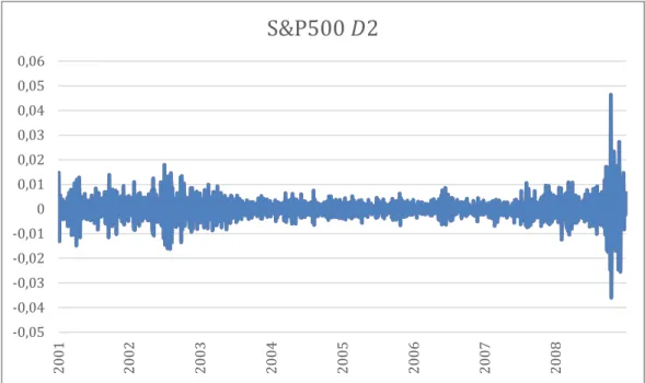
Figure 8- The blue line plots S&P500 OOS returns based on a 𝐷2 frequency brand which is obtained

from wavelet decomposition. This frequency captures the original time-series short-term behavior (4 to 8 days). -0,05 -0,04 -0,03 -0,02 -0,01 0 0,01 0,02 0,03 0,04 0,05 0,06 20 01 20 02 20 03 20 04 20 05 20 06 20 07 20 08

S&P500 𝐷2

48

Figure 9- The blue line plots the OOS GARCH (1,1) forecasts based on a S&P500 frequency 4-8 days (see graph Figure 8).

0,000% 0,050% 0,100% 0,150% 0,200% 0,250% 0,300% 0,350% 0,400% 0,450% 0,500% 20 01 20 02 20 03 20 04 20 05 20 06 20 07 20 08

GARCH 𝐷2