M A C RO E C O L O G I C A L M E T H O D S
Discrimination capacity in species
distribution models depends on
the representativeness of the
environmental domain
Alberto Jiménez-Valverde1*, Pelayo Acevedo1,2, A. Márcia Barbosa3,4, Jorge M. Lobo5and Raimundo Real1
1Department of Animal Biology, University of Málaga, Spain,2Department of Animal Health, Instituto de Investigación en Recursos Cinegéticos IREC, Ciudad Real, Spain,3‘Rui Nabeiro’ Biodiversity Chair, Centro de Investigação em Biodiversidade e Recursos Genéticos (CIBIO), University of Évora, Portugal,4Division of Biology, Imperial College London, UK,5Department of Biogeography and Global Change, Museo Nacional de Ciencias Naturales, Madrid, Spain
A B S T R A C T
Aim When faced with dichotomous events, such as the presence or absence of a species, discrimination capacity (the ability to separate the instances of presence from the instances of absence) is usually the only characteristic that is assessed in the evaluation of the performance of predictive models. Although neglected, cali-bration or reliability (how well the estimated probability of presence represents the observed proportion of presences) is another aspect of the performance of predic-tive models that provides important information. In this study, we explore how changes in the distribution of the probability of presence make discrimination capacity a context-dependent characteristic of models. For the first time, we explain the implications that ignoring the context dependence of discrimination can have in the interpretation of species distribution models.
Innovation In this paper we corroborate that, under a uniform distribution of the estimated probability of presence, a well-calibrated model will not attain high discrimination power and the value of the area under the curve will be 0.83. Under non-uniform distributions of the probability of presence, simulations show that a well-calibrated model can attain a broad range of discrimination values. These results illustrate that discrimination is a context-dependent property, i.e. it gives information about the performance of a certain algorithm in a certain data population.
Main conclusions In species distribution modelling, the discrimination capacity of a model is only meaningful for a certain species in a given geographic area and temporal snapshot. This is because the representativeness of the environmental domain changes with the geographical and temporal context, which unavoidably entails changes in the distribution of the probability of presence. Comparative studies that intend to generalize their results only based on the discrimination capacity of models may not be broadly extrapolated. Assessment of calibration is especially recommended when the models are intended to be transferred in time or space.
Keywords
Area under the ROC curve, calibration, classification, contingency matrix, discrimination, probability, reliability, species distribution modelling, uncertainty.
*Correspondence: Alberto Jiménez-Valverde, Department of Animal Biology, University of Málaga, 29071 Málaga, Spain.
E-mail: [email protected] and [email protected]
I N T RO D U C T I O N
Models, as simple representations of a complex world, make possible the quantification and understanding of natural phe-nomena and the generation of predictions (Soetaert & Herman, 2009). Predicting dichotomous events is necessary in a variety of every-day situations ranging from assessment of the quality of a wine to diagnostic medicine (Swets et al., 2000). In the fields of ecology, biogeography and evolution, predicting species occur-rence (species distribution modelling, herein SDM; for recent reviews see Franklin, 2009; Peterson et al., 2011) has become an important approach in overcoming what has been called the Wallacean shortfall, i.e. the general lack of knowledge about the distribution of species (Whittaker et al., 2005).
For models to be considered useful, they need to be evaluated (Rykiel, 1996). Usually, predictive performance is the only facet on which researchers focus their attention, and it is desirable that the predictions match the observations as closely as possi-ble. When faced with a dichotomous event, the most common practice is to assess discrimination capacity, i.e. the effectiveness of the scoring rule (S; usually called suitability in SDM) for separating the positive (instances of presence of the species, Y= 1) from the negative (instances of absence of the species, Y= 0) outcomes (Harrell et al., 1984). The area under the receiver operating characteristic (ROC) curve (AUC) has been a widely adopted statistic in measuring discrimination power (Hilden, 1991; Swets et al., 2000; Lobo et al., 2008; for extensive details on the ROC analysis see Krzanowski & Hand, 2009). The AUC can be interpreted as the probability P(S|Y= 1> S|Y = 0), i.e. the probability that a positive case chosen at random will be assigned a higher S than a negative case chosen at random. Therefore, what is important for the AUC is the ranking of the S-values, not their absolute difference. This simple interpreta-tion has probably contributed to its widespread use, though it is not exempt from criticism (Hilden, 1991; Lobo et al., 2008; Peterson et al., 2008; Jiménez-Valverde, 2012). In this study, the AUC will be used to account for discrimination as it is a common statistic and because our results do not depend on the metric used but are relevant for any discrimination measure.
If S is expressed as probability of presence, then the calibra-tion of the model is an addicalibra-tional aspect of predictive perform-ance that should be assessed (note that transformations of S can be used to recalibrate any kind of scoring rule; see Thomas et al., 2001). Calibration has different meanings; in statistics, the most widely used meaning refers to the model fitting process. In this study, we understand calibration (or reliability) as the degree to which the observed proportion of positive cases (empirically estimated probabilities) equates to the model estimated prob-abilities in any given testing data set (Harrell et al., 1984; Hosmer & Lemeshow, 2000). In a well-calibrated model, P(Y= 1|S)= S. For instance, in a SDM context, one would want 80% of the locations predicted with a probability of 0.8 to be occupied by the focus species. The calibration graph, in which P(Y= 1|S) is plotted as a function of S, is an easy way to assess calibration (Harrell et al., 1996); the graph of a perfectly calibrated model will match the identity (45°) diagonal (for further details see
Sanders, 1963; Pearce & Ferrier, 2000). Calibration and discrimi-nation are two aspects of a multi-sided general concept, that is, prediction performance (Sanders, 1963; Miller et al., 1991; Pearce & Ferrier, 2000). Although they refer to different qualities of the models, a priori, some constraints and trade-offs exist, and calibration and discrimination are not entirely independent from each other (Murphy & Winkler, 1992). For instance, the reader may have already realized that, at first glance, a perfectly calibrated model cannot achieve perfect discrimination (Diamond, 1992).
Pearce & Ferrier (2000) were the first to formally introduce the calibration concept in the SDM field. These authors dis-cussed the differences between discrimination and calibration, explained how to measure and interpret the calibration of models and illustrated how the two concepts tell us different things about the performance of models. Recently, Phillips & Elith (2010), inspired by Hirzel et al. (2006), have suggested a way to approximate a calibration curve when no absence records are available, a common situation in biodiversity studies. Under this scenario of lack of absence data, the empirical probabilities cannot be estimated, so the calibration plot cannot be built. Under certain strong assumptions, the presence-only calibration (POC) plot devised by Phillips & Elith (2010) may be a way to deal with this shortcoming. Unfortunately, apart from these commendable efforts, and contrary to what happens in other scientific domains, few authors in SDM have paid attention to calibration, while most of them have focused just on discrimination.
In this study, we describe the basic relationships that exist between calibration and discrimination and show, using easy-to-understand simulations, that for these relationships to hold, uniformity in the distribution of S is a necessary assumption. We explore in depth how non-uniformity in the distribution of S indicates that discrimination capacity is a context-dependent characteristic of models. For the first time, we fully explain the dramatic implications that ignoring the context-dependence of discrimination can have in the interpretation of species distri-bution models.
C A L I B R A T I O N A N D D I S C R I M I N A T I O N : B A S I C P A T T E R N S A N D TR A D E - O FF S
Two points need to be emphasized before proceeding. First, throughout this paper it is assumed that there is reliable infor-mation about the positive as well as the negative cases, at least for model evaluation. As said before, because of the increasing avail-ability of presence data in digital biodiversity databases, in the last few years there has been a notable interest in developing ways of predicting species distributions without using absence data. Instead, pseudo-absences (a sample of locations with no information about the presence or absence of the species) or background data (a sample of locations representing the envi-ronmental variation of the study area) are often used together with presence data for model training and evaluation (see Peter-son et al., 2011; but see Royle et al., 2012). However, without absence data for model testing, the application of discrimination
measures such as the AUC is questionable (Jiménez-Valverde, 2012). In addition, calibration can only be properly assessed if reliable absence data allow the estimation of the observed prob-ability P(Y = 1|S). Second, the evaluation of models can be performed at different levels. On one extreme, the accuracy of models can be assessed only on the training data, i.e. using entirely non-independent data. On the other, the interest may lie in testing the model under completely different circumstances using independent data (for example, from a different region or time). In between, there is a continuum in the degree of inde-pendence of the testing data set, and the researcher has to choose the level of independence according to the intended application of the model. Thus, throughout this paper, and unless stated explicitly, we will not refer to the degree of independence of the testing data and we will assume that it has been chosen properly according to the aim of the research; the revealed patterns and main conclusions are valid for any degree of independence.
That a perfectly calibrated model cannot attain perfect dis-crimination can be proved with a simple simulation exercise (see Appendix S1 in Supporting Information). A vector sjof S-values
was generated by picking a sample of n = 10,000 random numbers from a uniform distribution, j being the iteration number. A second vector wj, of the same length as sj, was
gener-ated in the same way. To create vector yjwith the information
about the outcomes of the binary event (e.g. the presence or absence of the focal species in SDM) the following condition was set:
ifwij<sijthenyij=1,elseyij=0,
where i denotes the cases (in SDM, the spatial locations) and ranges from 1 to 10,000. In this way, sjis a well-calibrated scoring
rule with respect to yj. The prevalence (i.e. the proportion of
positive outcomes in the sample) equals 0.5 because, given a perfectly calibrated model,
P Y( = =) P Y( = S f S S) ( ) = , −∞ ∞
∫
1 1 1 2 dwhere f(S) is the probability density function of S.
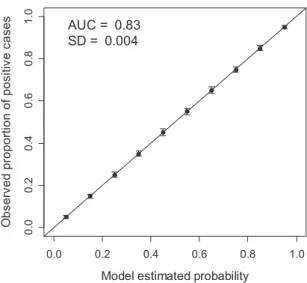
The AUC was computed using the ROCR (Sing et al., 2009) package for R (R Development Core Team, 2009). The proce-dure was repeated 100 times (j= {1, . . . , 100}) and the mean AUC was calculated (the simulation can be repeated by readers by copying and pasting the code of Appendix S1 in the R console). In Fig. 1 the results of the simulation are shown. The calibration plot shows that s is an almost perfectly calibrated prediction (it is not perfect because of the random sampling variation). To generate this plot, sjwas divided into 10 intervals
(bins, t= {1, . . . , 10}) of fixed cutpoints (following Lemeshow & Hosmer, 1982) so ntª 1000. Mean P(Y = 1|St) was plotted as a
function of mean stfor the 100 iterations (note that in the R
script provided in Appendix S1 only the last iteration is plotted as an example). A mean AUC value of 0.83 (SD⫾ 0.004) was obtained. Our simulation thus corroborates the result of Diamond (1992), who obtained the same AUC value for a per-fectly calibrated model via formal mathematical demonstration.
It is worth noting that a value of 0.83 does not represent ‘out-standing’ or ‘very good’ discrimination according to Hosmer & Lemeshow (2000) and Pearce & Ferrier (2000), respectively.
Extreme cases – note that these are not simulations but theo-retical constructs – are idealized in Fig. 2. When the calibration departs from perfection and the model overestimates P(Y= 1|St)
for the bins below certain t and underestimates P(Y = 1|St)
for the bins above that t (Fig. 2a), then discrimination cap-acity increases and the AUC exceeds the base 0.83 value (0.83< AUC < 1). In the reverse situation, when the model underestimates P(Y = 1|St) for the bins below certain t and
overestimates P(Y= 1|St) for the bins above that t (Fig. 2b),
discrimination capacity decreases and the AUC falls behind the base 0.83 value (0.5< AUC < 0.83). Note that a global calibra-tion index based on squared errors would yield the same value for both scenarios depicted in Fig. 2(a) and (b). If P(Y= 1|St)=
1 for every bin above certain t and P(Y= 1|St)= 0 for every bin
below that t (Fig. 2c), then discrimination is perfect and AUC= 1. In the reverse situation, when P(Y= 1|St)= 0 for every bin
above certain t and P(Y= 1|St)= 1 for every bin below that t
(Fig. 2d), then AUC= 0. Note that AUC values below 0.5 mean that the model is useful for discrimination but not for ranking, i.e. it is using the information in the inverse way (Fawcett, 2006), so an AUC of 0 also means perfect discrimination. If P(Y= 1|St)
is constant for every t (Fig. 2e), then discrimination is no better than chance and AUC = 0.5. The last situation refers to the scenario in which P(Y= 1|St)= 1 for some bins and P(Y = 1|St)
= 0 for the others but, contrary to the cases shown in Fig. 2(c) and (d), the bins show an alternating pattern (Fig. 2f). In this
0.0 0.2 0.4 0.6 0.8 1.0 0 .0 0 .2 0 .4 0 .6 0. 8 1 .0
Model estimated probability
s es ac evi ti s o p f o n oit r o p or p d ev r es b O AUC = 0.83 SD = 0.004
Figure 1 Calibration plot of the simulations showing the mean model estimated probability (x-axis) against the mean observed proportion of positive cases (y-axis) for 10 equal-size probability intervals (bins) and 100 iterations (see text for details). The graph shows that the simulated scoring rules are almost perfectly calibrated, whereas the mean area under the receiver operating
characteristic (ROC) curve (AUC) is 0.83 (SD⫾ 0.004). Solid line:
identity line indicating perfect calibration; whiskers: standard deviation.
case, the AUC can have any value between 0 and 1. For instance, in a forecast with a calibration plot like the one shown in Fig. 2(f), where P(Y= 1|St)= 0 and P(Y = 1|St)= 1 alternate one
at a time and P(Y= 1|S1)= 0, the AUC equals 0.6. The interesting point to highlight here is that, although the AUC is always lower than 1 (i.e. ranking is not perfect), this sort of scoring rules perfectly resolves the classification task of separating the positive from the negative outcomes (Hilden, 1991; Flach, 2010). Although these scenarios may not be common (especially in cases in which S has a natural order such as in probabilistic models), spotting them may help to detect and understand
the effect of new interactive factors that condition the outcome of the event (see Appendix S2).
B RE A K I N G D O W N T H E TR A D E - O FF S : D I S C R I M I N A T I O N D E P E N D S O N T H E D I S T R I B U T I O N O F S
The AUC value equals 0.83 in a perfectly calibrated model if and only if ntis constant for every bin. To show the
implica-tions of the violation of this condition, we ran simulaimplica-tions (see pseudocode in Appendix S3) in which, starting from an almost
Figure 2 Different idealized calibration plots of scoring rules that deviate from perfect calibration, and their relationship with discrimination (the sample size is the same for every bin). (a) Better discrimination than a perfectly calibrated model [area under the receiver operating characteristic curve (AUC) higher than the base value of 0.83]. (b) Worse discrimination than a perfectly calibrated model (AUC lower than the base value of
0.83). (c) Perfect discrimination (AUC=
1). (d) Perfect discrimination, but the scoring rule is using the information in the wrong way (low values correspond to positive outcomes and high values correspond to negative outcomes,
AUC= 0). (e) Discrimination is no
better than chance (AUC= 0.5).
(f) Perfect discrimination, but the AUC is lower than 1.
perfectly calibrated scoring rule (n= 10,000), ntwas
progres-sively reduced (see Fig. 3). First, sjand yjwere created as
out-lined in the previous section. Second, nt was decreased in
certain bins to nª 15 [nt was maintained (ntª 1000) in the
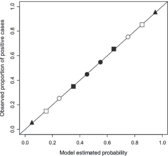
remaining bins], as 15 seems to be the minimum sample size necessary to estimate P(Y = 1) with admissible accuracy (Jovani & Tella, 2006). A first ‘set A’ of simulations was run in which the bins that were reduced followed the scheme: t= 5 and t= 6 (level 1); t = 4, t = 5, t = 6 and t = 7 (level 2); t = 3, t= 4, t = 5, t = 6, t = 7 and t = 8 (level 3); t = 2, t = 3, t = 4, t= 5, t = 6, t = 7, t = 8 and t = 9 (level 4). In a second ‘set B’, the reduction pattern was as follows: t= 1 and t = 10 (level 1); t= 1, t = 2, t = 9 and t = 10 (level 2); t = 1, t = 2, t = 3, t = 8, t= 9 and t = 10 (level 3); t = 1, t = 2, t = 3, t = 4, t = 7, t = 8, t= 9 and t = 10 (level 4). In total, 800 simulations were run (100 iterations¥ 2 sets ¥ 4 levels). The AUC was computed for each iteration and a mean AUC value was obtained for each level on each set. To assess calibration, the Hosmer–Lemeshow goodness-of-fit statistic (H-L; Lemeshow & Hosmer, 1982) was calculated for each iteration and a mean H-L was obtained for each level on each set.
The results showed that, although calibration did not change (Fig. 4a), the AUC significantly varied from level to level (Fig. 4b), ranging from 0.59 (⫾ 0.012) to 0.96 (⫾ 0.005). The AUC increased as sample size was reduced in the intermediate bins (set A); in contrast, it decreased as sample size was reduced in the outermost bins (set B).
G E N E R A L D I S C U S S I O N
The existence of a trade-off between calibration and discrimi-nation is not a new point (Murphy & Winkler, 1992). Under ideal conditions, increasing calibration compromises discrimi-nation in the sense that it is impossible to achieve perfect cali-bration and perfect discrimination if the sample size is constant for every bin (Diamond, 1992). Thus, under a uniform distri-bution of S, a perfectly calibrated model will yield an AUC of 0.83 (Fig. 1). Considering this base discrimination value, multi-ple discrimination–calibration combinations are possible and only deviations from perfect calibration will yield AUC values closer to 1 (Fig. 2). However, as we have shown in this study, the relationship between calibration and discrimination becomes complicated if the sample size differs among probability inter-vals (i.e. non-uniform distributions of S), which is commonly the case. In fact, if S= 0 for every negative case and S = 1 for every positive case, then the scoring rule will be perfectly cali-brated and will have a perfect discrimination capacity (AUC= 1). However, the predictions of such a model would be highly uncertain (Murphy & Winkler, 1992) aside from the fact that this is a very unlikely situation in real-world SDM scenarios. Complete separation of the outcomes is a well-known problem in statistical model fitting, as it avoids the correct estimation of the parameters (Lesaffre & Albert, 1989), producing uninforma-tive models.
In the second edition of their seminal work on logistic regres-sion, Hosmer & Lemeshow (2000) already noted that discrimi-nation depends on the distribution of the probabilities, and warned that discrimination measures coming from a 2¥ 2 con-tingency matrix (e.g. sensitivity, commission rate and others; for a review see Fielding & Bell, 1997) cannot be used to compare model performance (Hosmer & Lemeshow, 2000, pp. 158–160). Here, using simulations and the AUC as a threshold-independent measure, we have demonstrated this point, a fact that is far from trivial. The same model can be unsoundly quali-fied as ‘bad’, ‘good’ or ‘excellent’ – from a discrimination capacity point of view – depending on the distribution of the S-values. Discrimination is thus context specific, i.e. it depends on the configuration of the testing data set. This will happen even if the model is equally well (or badly) calibrated in the different con-texts. In the field of SDM this has two very important implica-tions, which we discuss below.
First, it explains the devilish effect of the geographic extent (or geographic background) raised by Lobo et al. (2008) and Jiménez-Valverde et al. (2008), which results in a negative rela-tionship between the relative occurrence area (the extent of the area occupied by the species relative to the total extent of the study area) and discrimination capacity. For the same total geo-graphic extent, and due to the frequent spatial autocorrelation among environmental variables (Legendre, 1993), the size of the species’ occurrence area conditions the distribution of the S-values in such a way that small areas bias S towards extreme values. This is the main reason why rare species usually yield higher discrimination values than widespread species, even though the models may be equally well (or ill) calibrated for
0.0 0.2 0.4 0.6 0.8 1.0 0. 0 0 .2 0. 4 0 .6 0. 8 1 .0
Model estimated probability
s es ac evi ti s o p f o n oit r o p or p d ev r es b O 0.0 0.2 0.4 0.6 0.8 1.0 0. 0 0 .2 0. 4 0 .6 0. 8 1 .0
Model estimated probability
s es ac evi ti s o p f o n oit r o p or p d ev r es b O
Figure 3 Scheme of the simulations performed to show the dependence of discrimination on the distribution of the probabilities. A first ‘set A’ of simulations was run in which the
bins that were reduced followed the scheme:
•
(level 1);•
and䊏 (level 2);•
,䊏 and 䊊 (level 3);•
,䊏, 䊊 and 䊐(level 4). In a second ‘set B’, the reduction pattern was as follows: 䉱 (level 1); 䉱 and 䊐 (level 2); 䉱, 䊐 and 䊊 (level 3); 䉱, 䊐, 䊊
both types of species. Precisely because discrimination is a context-dependent property, Jiménez-Valverde et al. (2008) concluded that the AUC should not be the only performance indicator used to compare distribution models between species, as the results may just be trivial (note that the same applies to any other discrimination measure). Most importantly, these authors stressed that higher discrimination values can be obtained simply by increasing the geographic extent of analysis (see also Barve et al., 2011; Acevedo et al., 2012), a fact that compromises the robustness of many SDM studies.
A second and less apparent consequence is that discrimina-tion may not be used to compare different modelling techniques for the same data population and to draw general conclusions beyond that population. Different techniques will be parameter-ized in different ways, yielding different distributions of S and, therefore, different discrimination values. A priori, there is no reason to assume that these differences in the distributions of S between techniques will be consistent among case studies/data populations. Discrimination capacity is an entirely context-dependent property; therefore, generalizations based on any dis-crimination statistic are unfounded. A ‘good’ or ‘bad’ model – from a discrimination point of view – can be qualified as ‘good’ or ‘bad’ only in the specific situation in which it was evaluated. In SDM, this means that discrimination is only informative in a concrete spatial, temporal and taxonomic context. This happens because the representativeness of the environmental domain changes with the geographical and temporal context, which unavoidably entails changes in the distribution of S. Broad com-parisons of models based only on discrimination statistics that aim to find the ‘best’ algorithm for every situation and taxon are flawed (see also Terribile et al., 2010). Statisticians know that no classification method can be universally advocated, and that the improved performance of new complex techniques may not be as relevant or useful as it may seem at first (Hand, 2006, and references therein). So, the weight given to the modelling tech-nique in SDM may be, on most occasions, unjustified. As pointed out by some authors, data quality is probably the most important factor influencing general model performance, an aspect to which much more effort and resources should be
devoted (Lobo, 2008; Jiménez-Valverde et al., 2010; Feeley & Silman, 2011; Rocchini et al., 2011).
The relevance of discrimination or calibration will depend on the intended application of the model (Pearce & Ferrier, 2000; Vaughan & Ormerod, 2005). If the ranking or the classification of the cases in a specific context (i.e. in a concrete data popula-tion) is the main interest, then discrimination capacity is impor-tant and may be an appropriate criterion for selecting the best model. But if the quantitative value of S is of interest, then calibration should be preferred. The probability values contain information about the uncertainty of the predictions (Keren, 1991; Murphy & Winkler, 1992). A well-calibrated model will give the probability that a certain case has to show the event, i.e. in an SDM study, it will tell us the probability of a location containing the focal species. It has been argued that, for some applications in SDM, it could be useful to convert probability maps into categorical (presence/absence) maps (Jiménez-Valverde & Lobo, 2007). Whether this is useful or not, this con-version implies the loss of information about the uncertainty of the predictions; this fact suggests the adequacy of publishing the probability maps at least as online supplementary material. Given a case with the event and another case without the event, the AUC will tell us the probability that both cases have of being correctly classified, but it will say nothing about the concrete cases or about the uncertainty of their predicted values (Hilden, 1991; Matheny et al., 2005). For two pairs of cases (0, 1), one with S-values (0.49, 0.51) and the other with S-values (0.2, 0.8), discrimination is perfect in both instances (for a threshold value of 0.5); yet, the uncertainty in the classification of these cases is not the same and the information that the S-values contain is of much more worth than that yielded by the binary classification. Following this line of thinking, some authors have questioned the expediency of discrimination to evaluate models in a decision-making context (e.g. Coppus et al., 2009). In environ-mental management and assessment, ignoring the uncertainty in the predictions may compromise decision processes, with potentially negative consequences for both the focal species and the optimization of managing resources. In temporal and/or spatial transference situations (e.g. under a climate change
sce-Figure 4 (a) Mean Hosmer–Lemeshow goodness-of-fit statistic (H-L) values and (b) mean area under the area under the receiver operating characteristic curve (AUC) values of the simulated scoring rules. In ‘set A’, sample size is reduced from the midmost to the outermost probability intervals (bins); in ‘set B’, sample size is reduced from the outer-most to the midouter-most bins. Sample size is progressively reduced in four increasing depletion levels (see Fig. 3). Grey solid lines, mean value of the H-L statistic (a) and the AUC (b) for an almost per-fectly calibrated scoring rule; grey dashed lines and whiskers, standard deviations.
nario), and because discrimination is context specific, calibra-tion may provide more informacalibra-tion about the potential performance of the models.
C O N C L U S I O N S
Model discrimination capacity depends on the distribution of the scoring values. Therefore, it is a context-dependent charac-teristic and must be interpreted as such. Although we have focused on scoring values of a probabilistic nature, it is impor-tant to realize that this context dependence is also true for non-probabilistic S-values. This means that first, discrimination capacity says little about the general performance of the models, and second, the comparison of models based on discrimination capacity cannot be extended beyond a particular data popula-tion. Discrimination may be a property of interest if the mod-eller is interested in maximizing the capacity to separate the instances of presence from the instances of absence in a certain spatio-temporal context and data population. Calibration may be of more interest if the researcher is interested in transferring the model and producing more general conclusions.
Relying on a single summary discrimination measure to assess model performance may result in a loss of valuable information and lead to misleading conclusions. Discrimination measures should not be reported alone, but should always be accompanied with information about the distribution of the scoring values. Ideally, the ROC curve as well as the model calibration plots should be shown, explicitly indicating the sample size of each bin in the plot. Relatively small or large sample sizes in certain bins could explain the discrimination values obtained, and very low sample sizes could pinpoint uncertainty in the calibration assess-ment. Instead of using bins, smooth nonparametric calibration curves might be a better screening option (Harrell et al., 1996; Phillips & Elith, 2010). In this study we have used the H-L statistic to quantitatively assess calibration because it is a classical test and because our results do not depend on which statistic is applied. However, this statistic has well-known drawbacks (see, for instance, Lemeshow & Hosmer, 1982; Hosmer et al., 1997; Kramer & Zimmerman, 2007) that may discourage its use for assessing calibration. Other measures such as the unweighted-sum-of-squares statistic (Copas, 1989), Miller’s calibration sta-tistics (Miller et al., 1991; Pearce & Ferrier, 2000) or the coefficient of determination R2using the unity line (intercept= 0 and slope= 1) instead of the regression line (Poole, 1974, cited by Romdal et al., 2005, p. 238) may be preferred.
Finally, we would like to emphasize that our position is not to deny or demonize the use of discrimination measures for the assessment of model performance, but just to bring awareness of their limitations. The results presented here are of broad interest for any research(er) dealing with classification of dichotomous events. Taking into account the significance of the areas of research in which SDM is applied (see Peterson et al., 2011) and the widespread use of discrimination as the only way to assess model quality, the implications of our simulation study are noteworthy.
A C K N O W L E D G E M E N T S
The study was partially supported by projects CGL2009-11316/ BOS-FEDER and CGL2011-25544. A.J.-V. was supported by the MEC Juan de la Cierva Program. P.A. was supported by the Vicerrectorado de Investigación of the University of Málaga. A.M.B. was supported by a post-doctoral fellowship from Fundação para a Ciência e a Tecnologia (Portugal), co-financed by the European Social Fund. The ‘Rui Nabeiro’ Biodiversity Chair receives funding from Delta Cafés. Lucía D. Maltez kindly reviewed the English. Thanks to Paulo De Marco and another three anonymous referees for their constructive feedback.
R E F E RE N C E S
Acevedo, P., Jiménez-Valverde, A., Lobo, J.M. & Real, R. (2012) Delimiting the geographical background in species distribu-tion modelling. Journal of Biogeography, 39, 1383–1390. Barve, N., Barve, V., Jiménez-Valverde, A., Lira-Noriega, A.,
Maher, S.P., Peterson, A.T., Soberón, J. & Villalobos, F. (2011) The crucial role of the accessibility area in ecological niche modeling and species distribution modeling. Ecological Mod-elling, 222, 1810–1819.
Copas, J.B. (1989) Unweighted sum of squares test for propor-tions. Applied Statistics, Journal of the Royal Statistical Society Series C, 38, 71–80.
Coppus, S.F.P., van der Veen, F., Opmeer, B.C., Mol, B.W.J. & Bossuyt, P.M.M. (2009) Evaluating prediction models in reproductive medicine. Human Reproduction, 24, 1774–1778. Diamond, G.A. (1992) What price perfection? Calibration and discrimination of clinical prediction models. Journal of Clini-cal Epidemiology, 45, 85–89.
Fawcett, T. (2006) An introduction to ROC analysis. Pattern Recognition Letters, 27, 861–874.
Feeley, K.J. & Silman, M.R. (2011) Keep collecting: accurate species distribution modelling requires more collections than previously thought. Diversity and Distributions, 17, 1132– 1140.
Fielding, A.H. & Bell, J.F. (1997) A review of methods for the assessment of prediction errors in conservation presence/ absence models. Environmental Conservation, 24, 38–49. Flach, P.A. (2010) ROC analysis. Encyclopedia of machine
learn-ing (ed. by C. Sammut and G.I. Webb), pp. 869–875. Sprlearn-inger, New York.
Franklin, J. (2009) Mapping species distributions. Spatial infer-ence and prediction. Cambridge University Press, Cambridge. Hand, D.J. (2006) Classifier technology and the illusion of
progress. Statistical Science, 21, 1–15.
Harrell, F.E., Lee, K.L., Califf, R.M., Pryor, D.B. & Rosati, R.A. (1984) Regression modelling strategies for improved prog-nostic prediction. Statistics in Medicine, 3, 143–152.
Harrell, F.E., Lee, K.L. & Mark, D.B. (1996) Multivariable prog-nostic models: issues in developing models, evaluating assumptions and adequacy, and measuring and reducing errors. Statistics in Medicine, 15, 361–387.
Hilden, J. (1991) The area under the ROC curve and its com-petitors. Medical Decision Making, 11, 95–101.
Hirzel, A.H., Le Lay, G., Helfer, V., Randin, C. & Guisan, A. (2006) Evaluating the ability of habitat suitability models to predict species presences. Ecological Modelling, 199, 142–152. Hosmer, D.W. & Lemeshow, S. (2000) Applied logistic regression,
2nd edn. Wiley, New York.
Hosmer, D.W., Hosmer, T., le Cessie, S. & Lemeshow, S. (1997) A comparison of goodness-of-fit tests for the logistic regres-sion model. Statistics in Medicine, 16, 965–980.
Jiménez-Valverde, A. (2012) Insights into the area under the receiver operating characteristic curve (AUC) as a discrimina-tion measure in species distribudiscrimina-tion modelling. Global Ecology and Biogeography, 21, 498–507.
Jiménez-Valverde, A. & Lobo, J.M. (2007) Threshold criteria for conversion of probability of species presence to either–or presence–absence. Acta Oecologica, 31, 361–369.
Jiménez-Valverde, A., Lobo, J.M. & Hortal, J. (2008) Not as good as they seem: the importance of concepts in species distribution modelling. Diversity and Distributions, 14, 885– 890.
Jiménez-Valverde, A., Lira-Noriega, A., Soberón, J. & Peterson, A.T. (2010) Marshalling existing biodiversity data to evaluate biodiversity status and trends in planning exercises. Ecological Research, 25, 947–957.
Jovani, R. & Tella, J.L. (2006) Parasite prevalence and sample size: misconceptions and solutions. Trends in Parasitology, 22, 214–218.
Keren, G. (1991) Calibration and probability judgments: con-ceptual and methodological issues. Acta Psychologica, 77, 217– 273.
Kramer, A.A. & Zimmerman, J.E. (2007) Assessing the calibra-tion of mortality benchmarks in critical care: the Hosmer– Lemeshow test revisited. Critical Care Medicine, 35, 2052–2056.
Krzanowski, W.J. & Hand, D.J. (2009) ROC curves for continuous data. Chapman & Hall, Boca Raton, FL.
Legendre, P. (1993) Spatial autocorrelation: trouble or new para-digm? Ecology, 74, 1659–1673.
Lemeshow, S. & Hosmer, D.W. (1982) A review of goodness of fit statistics for use in the development of logistic regression models. American Journal of Epidemiology, 115, 92–106.
Lesaffre, E. & Albert, A. (1989) Partial separation in logistic discrimination. Journal of the Royal Statistical Society: Series B (Methodological), 51, 109–116.
Lobo, J.M. (2008) More complex distribution models or more representative data? Biodiversity Informatics, 5, 14– 19.
Lobo, J.M., Jiménez-Valverde, A. & Real, R. (2008) AUC: a mis-leading measure of the performance of predictive distribution models. Global Ecology and Biogeography, 17, 145–151. Matheny, M.E., Ohno-Machado, L. & Resnic, F.S. (2005)
Dis-crimination and calibration of mortality risk prediction models in interventional cardiology. Journal of Biomedical Informatics, 38, 367–375.
Miller, M.E., Hui, S.L. & Tierney, W. (1991) Validation tech-niques for logistic regression models. Statistics in Medicine, 10, 1213–1226.
Murphy, A.H. & Winkler, R.L. (1992) Diagnostic verification of probability forecasts. International Journal of Forecasting, 7, 435–455.
Pearce, J. & Ferrier, S. (2000) Evaluating the predictive perform-ance of habitat models developed using logistic regression. Ecological Modelling, 133, 225–245.
Peterson, A.T., Papes¸, M. & Soberón, J. (2008) Rethinking receiver operating characteristic analysis applications in eco-logical niche modelling. Ecoeco-logical Modelling, 213, 63–72. Peterson, A.T., Soberón, J., Pearson, R.G., Anderson, R.P.,
Martínez-Meyer, E., Nakamura, M. & Araújo, M.B. (2011) Ecological niches and geographic distributions. Princeton Uni-versity Press, Princeton.
Phillips, S.J. & Elith, J. (2010) POC plots: calibrating species distribution models with presence-only data. Ecology, 91, 2476–2484.
Poole, R.W. (1974) An introduction to quantitative ecology. McGraw-Hill, New York.
R Development Core Team (2009) R: a language and environ-ment for statistical computing. Version 2.10.1. R Foundation for Statistical Computing, Vienna, Austria. Available at: http:// www.R-project.org.
Rocchini, D., Hortal, J., Lenygel, S., Lobo, J.M., Jiménez-Valverde, A., Ricotta, C., Bacaro, G. & Chiarucci, A. (2011) Uncertainty in species distribution mapping and the need for maps of ignorance. Progress in Physical Geography, 35, 211– 226.
Romdal, T.S., Colwell, R.K. & Rahbek, C. (2005) The influence of band sum area, domain extent, and range sizes on the latitudinal mid-domain effect. Ecology, 86, 235–244. Royle, J.A., Chandler, R.B., Yackulic, C. & Nichols, J.D. (2012)
Likelihood analysis of species occurrence probability from presence-only data for modelling species distributions. Methods in Ecology and Evolution, 3, 545–554.
Rykiel, E.J. (1996) Testing ecological models: the meaning of validation. Ecological Modelling, 90, 229–244.
Sanders, F. (1963) On subjective probability forecasting. Journal of Applied Meteorology, 2, 191–201.
Sing, T., Sander, O., Beerenwinkel, N. & Lengauer, T. (2009) ROCR: visualizing the performance of scoring classifiers. R package version 1.0-4. Available at: http://CRAN.R-project.org/package=ROCR (accessed January 2011). Soetaert, K. & Herman, P.M.J. (2009) A practical guide to
eco-logical modelling. Springer, Dordrecht.
Swets, J.A., Dawes, R.M. & Monahan, J. (2000) Better decision through science. Scientific American, 283, 82–87.
Terribile, L.C., Diniz-Filho, J.A.F. & De Marco, P. (2010) How many studies are necessary to compare niche-based models for geographic distributions? Inductive reasoning may fail at the end. Brazilian Journal of Biology, 70, 263–269.
Thomas, L.C., Banasik, J. & Crooks, J.N. (2001) Recalibrating scorecards. Journal of the Operational Research Society, 52, 981–988.
Vaughan, I.P. & Ormerod, S.J. (2005) The continuing challenges of testing species distribution models. Journal of Applied Ecology, 42, 720–730.
Whittaker, R.J., Araújo, M.B., Jepson, P., Ladle, R.J., Watson, J.E.M. & Willis, K.J. (2005) Conservation biogeography: assessment and prospect. Diversity and Distributions, 11, 3–23.
S U P P O R T I N G I N F O R M A T I O N
Additional supporting information may be found in the online version of this article at the publisher’s web-site.
Appendix S1 R code for the simulation of binary events and almost perfectly calibrated scoring rules.
Appendix S2 Improper receiver operating characteristic curves.
Appendix S3 Pseudocode of the simulations.
B I O S K E T C H
Alberto Jiménez-Valverde is currently a Juan de la Cierva researcher at the University of Málaga. He is interested in broad-scale patterns of biodiversity and, particularly, in understanding the relative importance of environmental, biotic and historical factors in limiting species geographical ranges. He is also very interested in methodological and conceptual issues related to species distribution models, and in the ecology and biogeography of spiders.