Comparing two scale lengths in the context of a customer satisfaction survey

(1)

i

COMPARING TWO SCALE LENGTHS IN THE

CONTEXT OF A CUSTOMER SATISFACTION

SURVEY

Adriana Pereira Raupp

Dissertation presented as partial requirement for obtaining

the Master’s degree in Statistics and Information

(2)

i

NOVA Information Management School

Instituto Superior de Estatística e Gestão de Informação

Universidade Nova de Lisboa

COMPARING TWO SCALE LENGTHS IN THE CONTEXT OF A

CUSTOMER SATISFACTION SURVEY

by

Adriana Pereira Raupp

Dissertation presented as partial requirement for obtaining the Master’s degree in Information Management, with a specialization in Marketing Research and CRM

Advisor: Professor Pedro Coelho

(3)

i

ABSTRACT

In addition to tangible assets, nowadays, companies are being measured by their orientation towards customers. Thereby, organizations are making efforts to survey and understand their customers’ needs, which would result in customer satisfaction and ultimately bring competitive gains.

Customer satisfaction surveys can be done in several ways, within the various methodologies used across the world, since the 1990s. To this end, there are a couple industry standards in customer satisfaction measurement, such as the American and the European Customer Satisfaction indexes. Customers were surveyed in several attributes, which estimated other attributes that could culminate in the estimation of the satisfaction index. Indeed, this is done by using partial least squares structured equation modeling.

In this study, the methodology for the European Customer Satisfaction Index, ECSI, was applied to the customers of an online company in Brazil called Singu. Although, the ECSI methodology uses a scale length of ten points, in this work a five-point scale was used simultaneously, aiming at comparing the results obtained with both surveys and evaluating which one estimates best in this context. In the conclusion, results show why the longer scale is the best option in the end, in spite of having significant fewer respondents.

KEYWORDS

(4)

ii

INDEX

1. Introduction ... 1

1.1. Literature Review ... 2

2. Study Description ... 5

2.1. ECSI ... 5

2.2. Data ... 7

3. Results... 9

3.1. Rescaling ... 9

3.2. Descriptive Analysis ... 10

3.3. SEM Analysis ... 13

3.3.1. Reflective Model... 13

3.3.2. Structural Model... 17

4. Conclusion ... 23

5. Final Considerations ... 25

6. Bibliography ... 26

(5)

iii

LIST OF FIGURES AND TABLES

Figure 2.1 – SEM ECSI ... 6

Table 2.2 – Frequency ... 7

Table 2.3 – Demographic ... 8

Table 2.4 – Indicators ... 8

Table 3.1 – t Test for conversions ... 10

Table 3.2 – Mean ... 10

Table 3.3 – Skewness... 11

Table 3.4 – Kurtosis ... 12

Table 3.5 – Composite Reliability ... 13

Table 3.6 – Outer Loadings: Converted 5 ... 14

Table 3.7 – Outer Loadings: Original 10 ... 15

Table 3.8 – Average Variance Expected ... 15

Table 3.9 – Fornell Larcker: Converted 5 ... 16

Table 3.10 – Fornell Larcker: Original 10... 16

Table 3.11 – Inner VIF: Converted 5 ... 17

Table 3.12 – Inner VIF: Original 10 ... 17

Table 3.13 – Path Coefficients: Converted 5 ... 18

Table 3.14 – Path Coefficients: Original 10 ... 19

Table 3.15 – Total Effects: Converted 5 ... 19

Table 3.16 – Total Effects: Original 10 ... 19

Table 3.17 – P values: Path Coefficients ... 20

Table 3.18 – R square ... 20

Table 3.19 – Adjusted R square ... 21

Table 3.20 – f square: Converted 5 ... 21

Table 3.21 – f square: Original 10 ... 22

(6)

iv

LIST OF ABBREVIATIONS AND ACRONYMS

ECSI European Customer Satisfaction Index ACSI American Customer Satisfaction Index SEM Structured Equations Model

PLS Partial Least Squares KPI Key Performance Indicators AVE Average Variance Explained VIF Variance Inflation Factor

(7)

1

1. INTRODUCTION

Since the last decades, companies are being measured not only by their tangible assets, but also by their intangible assets. One of the most valuable intangible assets is the business methodology, especially when the processes inside a company are reoriented towards the customers´ needs, instead of focusing solely on the production end. This is a new paradigm for companies, being customer-centric, in the sense of understanding customers’ needs to satisfy them somehow, without compromising the company, resulting, ultimately, in competitive gains.

Market researches are a way of connecting the company to the customers via information, which is collected with instruments such as observation or survey. Customer satisfaction surveys can measure the satisfaction of product/service transactions post consume or it can measure the clients’ satisfaction as a whole, as a result of a cumulative process. The latter is able to measure the clients’ satisfaction in relation to the company (COELHO & VILARES, n.d.).

There are several ways of collecting responses in a survey; the option for one or another depends on the objectives and nature of the study. Scales are a very frequent approach to evaluate consumers’ preferences and characteristics; however even scales vary significantly in format.

These physical forms of representation of the answers are called the shape of scales. Response scales can be arranged in three major types: Verbal, Numerical, and Pictorial. Verbal scales are the most objective type of scale, since each point will be associated with a phrase, leaving the respondent free to choose and not having the need to make any association with each point. Because it needs to have a phrasing in each point, sometimes verbal scales lack in single dimensionality, which means the words chosen are not the same or exact opposites for each point, making it difficult for both the respondent and the analyst to interpret the question. A Likert scale is a famous verbal scale, usually used in the market research field to measure attitudes, commonly written with 5 points.

On the other hand, the use of numerical scales reduces the risk of the scale being multi-dimensional, since the words are substituted by numbers. However, the words chosen for describing the extremes must be in single-dimension. Another problem arises when this type of shape is selected: the level of interpretation customers will need to interpret the question may be higher due to the number of points between the anchored points in the extremes of the scale. The higher the number of points, the more difficult it is for the respondents to interpret and answer the question.

Some situations require a different shape of scale, in the form of images. A pictorial scale is mostly used when interviewing children or when the situation asks for more informality in the interview. Due to the subjective nature of this scale, best if used sparingly since it can render more difficult analysis. Pain is also usually measured with figures. Tools for measuring pain should be easy and quick, while at the same time efficient. Having simple tools for describing pain has benefits such as improving its relief, decreased measurement workload on people who should be treating (Hicks, Von Baeyer, Spafford, Van Korlaar, & Goodenough, 2001).

It might be considered easier to use a pictorial rating scale to measure subjective objects, for example pain, however, in a research it was proven that numerical rating scale with eleven points and verbal rating scale with 7 points also work well. What is most important is not the scale type, but other survey attributes that may interfere in the results, such as the wording of the extremes of the

(8)

2 scale, how the survey was administered, time frames, interpretation of the results, classification cut-offs, etc. (Hjermstad et al., 2011).

This dissertation aims to compare two of the traditional options in the field of rating scales, a five-point and ten-five-point length numerical scale, anchored in the extremes, in the context of a customer satisfaction survey. This will be done considering the critical analysis in the bibliography and previous research. It also aims to present the differences in the ability of interpretation and results of the statistical analysis between the two rating scales.

1.1. L

ITERATURE

R

EVIEW

Currently, due to the competitiveness between companies in different industries, it is becoming more difficult to build advantage. For this reason, companies are concentrating all efforts to satisfy customers, as it is considered that establishing customer-focused strategies is a way to have a better business performance (Ngo & Nguyen, 2016).

Therefore, it is important for companies to measure and evaluate the performance of a product or service, and to produce Key Performance Indicators (KPI) for the company from these evaluations. Training their employees to meet KPIs derived from market research is paramount (Lee & Park, 2015). Thus, changing the organization culture towards this purpose is imperative.

Nonetheless, the instrument for colleting customers’ evaluations is paramount for obtaining good result measurement. When designing a questionnaire, it is important to establish, among other features, the number of points on the scale used. There is no consensus in literature on the ideal length of scales for a market research survey (Friedman & Amoo, 1999).

Longer scales tend to estimate better the respondent’s evaluation of each attribute, due to smaller intervals. But, what shorter scales lack in precision, they gain in less effort from the respondents, generating larger amount of responses, which produces better quality results (Coelho & Esteves, 2007).

It is necessary to find a balance between the possibility of having discriminated responses and the effort requested from the interviewee. Further, when designing a survey, one need to consider that the larger the scale, the more variability the responses will have, which can compromise the accuracy of the results, since the distribution of answers will be more scattered (Dawes, 2008). At the end, there is a tradeoff between increase in accuracy, by using a smaller scale, and increase in precision, by adding points in a scale (Friedman & Amoo, 1999).

The larger the scales in a survey, the more variability and the more reliability the results will have. In addition to this, finer scales produce less kurtosis due to larger variance (Dawes, 2008). This is ideal, since transforming a data set with the objective of normalizing it always risks losing information. Another fact a researcher has to take into consideration is that Likert scales tend to show negative skew, which may also influence statistical analysis and could require normalization of data (Peterson & Wilson, 1992).

(9)

3 The subject under study influences the optimal number of points. Previous research concluded that a choice from 5 to 11 points is generally best. If the object being rated does not require a high level differentiation, even 3 points could be appropriate, yet, surveys measuring behavior or perception should use larger scales (Friedman & Friedman, 1986).

Furthermore, one has to decide if the scale used should have even or odd numbers. If using the even option on a study, respondents can select the middle point because they are genuinely indifferent to the topic or because they do not want to answer the question. Some authors have concluded on this matter that, when there are middle points in a scale, it is usually oversampled.

However, sometimes when applying a questionnaire, there are some topics where people genuinely do not have experience or opinion on it, so in these cases they can choose an alternative option which is “do not know” or other similarly constructed sentence. By adding this option as a possible answer, it would allow for more meaningful responses, when forced to choose without experience, responses are less accurate (Friedman & Amoo, 1999). If researchers choose to include this option though, one should be careful in not adding it in the most important question of the survey, since it is imperative to have a concrete response on the specific characteristic or object under study.

A popular belief is that people from various socio-demographic backgrounds would have different ease with varying scale lengths, but it was shown that this is not true. Researchers must consider carefully the wording when developing a questionnaire, but it has been proven that both a survey with a 5 or a 10-point scale have resulted in similar non-response rates and mean scores, which indicates that these scale lengths do not increase the effort of the respondent (Coelho & Esteves, 2007).

Regarding the description of the points, there are several options; it is possible to define only the anchors of the scale, or all of the points, or even define the points as the description, i.e., without a number associated. There have been some discussions about if adding or not the labels on the scale. Some of them argue that, if not labeled, it will increase the measurement error, by cause of the respondent making their own inferences, which might be different from the researchers’. There are no statistical impacts between a fully described or anchored scales (Eutsler & Lang, 2015).

In addition, it is also important to select carefully the category descriptors; they should depend on the target audience. Not only the target population must be familiar with the wording used, but the adjectives chosen are also a tool to compute means and parametric statistics to make further analysis. The interpretation of the anchors has to create equal-interval frequency scales. Some adjectives can unbalance a scale that is supposedly balanced, not using the same adjective to anchor the extremes, for example, or using similar but not equal adjectives. When evaluating customer perceptions, numbers associated with points can also influence the respondents, the impact of negative numbers is very strong compared to a scale of 0 to 10 (Friedman & Amoo, 1999).

Furthermore, when choosing a medium to apply customer satisfaction questionnaires, one has to consider other factors, such as budget and target population. At a very low cost and broad reach, online surveys sent by email have a great advantage over traditional media, such as telephone or post. A direct result of the reach and the easiness to fill the questionnaire is that the response rate is

(10)

4 usually higher (Ilieva, Baron, & Healey, 2002) and faster (Gunter, Nicholas, Huntington, & Williams, 2002).

How to reach a target population is important because it depends on the characteristics of such population. In the past, online surveys were not considered optimal (Gunter et al., 2002) since fewer people had access to the internet. Sixteen years later, this is less relevant for a company that provides online services exclusively, yet one could argue that this population could have become more diverse.

The way to evaluate online companies differs from traditional markets. A study has shown that, although initially, price was considered the main driver, it is less relevant on assessing an e-business success than satisfaction with the quality of service. Due to this, new technical dimensions need to be considered in the Perceived Quality construct, such as user experience and interface (Hsu, 2008).

(11)

5

2. STUDY DESCRIPTION

The data for this work was collected as a customer satisfaction survey on the company Singu. It is a mobile service company that operates in the Brazilian market by connecting beauty professionals to clients via an app for mobile phones. At the moment, the services offered are three and the coverage is limited to the city centers of Rio de Janeiro and of São Paulo. They have been operating for about 2 years and currently have a database of clients of around 15,000.

The target population used was the clients of the company under study who have used at least one service, at least one time.

Two surveys were developed following the methodologies described in Section 2.2. In order to guarantee quality to the research, data was collected from the target population in three moments: an exploratory research, to refine customer perceptions of the service; a pilot questionnaire (for both types of researches, exploratory and conclusive) to test the questions, the flow, and the understanding by respondents; and a conclusive research, when the results were quantified and then analyzed.

The research and the statistical analysis follows the European Customer Satisfaction Index, (ECSI), which is a tested and successful methodology used all over European countries and the rest of the world. The methodology consists of 27 indicators with 7 latent variables, and estimation is done using a Partial Least Squares (PLS) applied to a Structural Equation Model (SEM). ECSI uses a 10-point scale. In order to compare the results obtained with different scales, the questionnaires were not only adapted to the context of the Brazilian language and culture, but adapted to the context of this particular company, which is not a sector currently analyzed by ECSI, and to the use of a 5-point scale.

The tools used to analyze data for this work were SAS and SmartPLS (Ringle, Wende, & Becker, 2015).

2.1. ECSI

The methodological approach for this work was based on ECSI. Companies that use ECSI can better predict the company's future results, especially when considering the loyalty attribute, to better diagnose satisfaction issues. The intrinsic model to be applied is able to: (a) explain and quantify the variables involved in satisfaction estimation; (b) better integrate all areas of the company by using an approved methodology; and (c) produce better benchmarks, as comparison inside and outside of the industry is easier, since data of others companies are available.

ECSI contains sets of causal relationships, and can indicate the relationship between the antecedents (customer expectations, perceived service quality, image and perceived value) and the consequences (satisfaction, customer complaints and customer loyalty) of customer satisfaction (Deng, Yeh, & Sung, 2013), as we can observe in Figure 2.1, with antecedents in blue color and consequences in yellow color.

(12)

6 Figure 2.1 – SEM ECSI

The methodological approach for the ECSI model is structural, probabilistic and simultaneous. A structured approach means that different attributes will have different weights in the estimation of the satisfaction of clients. And each of these attributes, named latent variables, is estimated by specific indicators. The indicators are the questions of the survey. In general, there are twenty-seven indicators, which can estimate 7 attributes of the company: image, expectation, perceived quality, perceived value, satisfaction, loyalty and complaints. Some of these influence just one attribute, but others may influence up to three attributes, e.g. Expectations construct only influences Satisfaction while Image and Perceived Value influence three constructs each: Loyalty, Satisfaction and Perceived Value, the former, and Satisfaction, Expectations and Perceived Quality, the latter.

The probabilistic approach means that the model uses a sample and it generalizes the results for the whole population, avoiding extra expenses in surveying the entire population. Furthermore, the model is estimated simultaneously, since it recognizes the interdependence nature of the estimation of the attributes, for both exogenous and endogenous latent variables. As opposed to estimating each relationship at a time, the simultaneous model considers all possible relationships at the same time, thus estimating better parameters.

The scale format used on ECSI surveys are ten-point, previous study comparing this to a 5-point scale showed similar results, but it compared two surveys done by random digit dialing, in Portugal. The present study aims to compare the same two lengths on surveys applied via internet forms. The analysis done on this study was not focused on how socio-demographic characteristics could affect the results, but more on the data characteristics itself.

(13)

7

2.2. D

ATA

The surveys were done online, which is cheapest and fastest way of collecting the most quantity of data. The tool used was Google Forms, which is a free, with no limitations in both format and data size. The questionnaires were exactly the same for both surveys; the only difference was the scale length. Respondents had between the 29th of November 2017 to 11th of December 2017 to answer the survey, and were limited to sending their answer only one time, to avoid bias.

The sampling frame was provided by the company, as it has a database with the registered emails of all users of the app. The emails were divided randomly into two mailing lists and each received a link to one of the surveys along with an explanation letter.

Since there is a possibility that some app users may have registered their email with the company and not used any service, it was necessary to have a qualifying question. To this end, the target population filter used was “How many times have you used the app?”. If the answer was “Never”, the survey would end up there. All other type of answers to this question would qualify for continuing to answer the survey.

Each questionnaire form was sent to around 11,500 users. The questionnaire using the scale of five points had 319 responses, while the one with ten points had 209. We should consider the evaluations of the surveyed customers relevant since more than 70% of them have used the services of the company more than once, hence accumulating experiences and not evaluating based on one sole opportunity. Table 2.2 shows the frequency in percentages that the customers used or not the company’s service for both forms.

Original 5 Original 10 1 time 23.8% 25.4% 2 to 5 times 48.9% 51.7% 6 or more 25.7% 19.1% Never 1.6% 3.8% Table 2.2 – Frequency

After filtering for only those respondents who have used the service of the company at least once, 314 customers were surveyed using the five-length scale and 201 on the ten-length. In Table 2.3, we can see how similar both populations are, especially when considering the most significant users in quantity, from age 26 to 45, which represent, in both, more than 70%. Also, in Table 2.3, we can see the percentages of the gender of the population that preferred to answer about it.

Original 5 Original 10 Less than 18 years 0.3% 0.0% 18 to 25 years 22.6% 15.9% 26 to 35 years 55.4% 58.7% 36 to 45 years 17.2% 17.9% 46 to 55 years 2.5% 3.0% 56 to 65 years 1.9% 4.0% More than 65 0.0% 0.5%

(14)

8 years

Female 98.1% 99.0%

Male 1.6% 0.5%

Prefer not to say 0.3% 0.5% Table 2.3 – Demographic

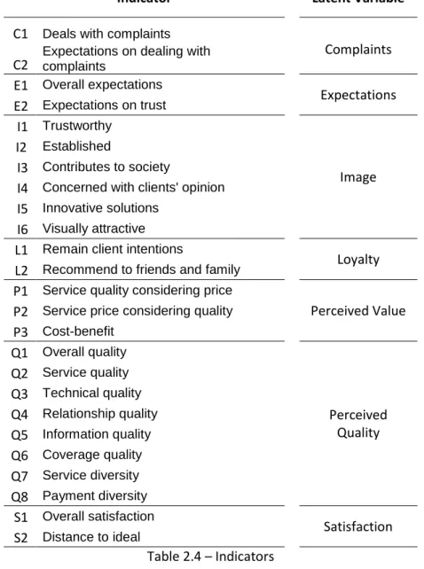
Aside from the qualification question and the demographic questions, the questionnaire was built considering the latent variables of the ECSI model. In Table 2.4 there is a list of the indicators and the corresponding latent variables, showing what the questions intended to measure. The indicators aim to reflect the latent variables that are not possible to be measured directly.

Indicator Latent Variable

C1 Deals with complaints

Complaints C2 Expectations on dealing with complaints

E1 Overall expectations Expectations E2 Expectations on trust I1 Trustworthy Image I2 Established I3 Contributes to society

I4 Concerned with clients' opinion

I5 Innovative solutions

I6 Visually attractive

L1 Remain client intentions

Loyalty L2 Recommend to friends and family

P1 Service quality considering price

Perceived Value P2 Service price considering quality

P3 Cost-benefit Q1 Overall quality Perceived Quality Q2 Service quality Q3 Technical quality Q4 Relationship quality Q5 Information quality Q6 Coverage quality Q7 Service diversity Q8 Payment diversity S1 Overall satisfaction Satisfaction S2 Distance to ideal Table 2.4 – Indicators

(15)

9

3. RESULTS

3.1. R

ESCALING

In order to compare both 5-point and 10-point studies, the scales needed to have the same size. The rescaling was done, at first, by converting the both extremes of the five-length scale in 1 and 10, then, the middle point, 3, was converted to a 5, however, in the end this showed to be a poor conversion.

A new results table was created, with the difference between the values of the ten-length scale and the five-length converted for all the variables. With the new results, a T test was run on the averages of each variable to verify if the difference between the surveys was statistically significant or not, at a 90% significance level.

As mentioned, the conversion was poor due to the fact that the five-length converted was significantly negatively biased in five variables: I2, Q5, C1, C2 and S2.

In light of this, the change was made to the middle point rescaling. The rescaling was done at the actual middle point of the scale, the third point of the five-length scale became a 5.5, the second point was transformed in a 3.25 and the fourth point is now a 7.75 (Dawes, 2008) . When testing the difference for the ten-length scale to the newly converted five-length, the results were significantly more balanced. At a 90% confidence level, only two variables were statistically different: I1 and I2.

Variable Pr >|t| 5 Pr >|t| 5.5 S1 0.3879 0.9764 I1 0.2285 0.0529 I2 0.0003 0.0349 I3 0.2522 0.9179 I4 0.5507 0.9426 I5 0.2800 0.9607 I6 0.1174 0.6938 E1 0.1902 0.7004 E2 0.8274 0.3212 Q1 0.4736 0.7982 Q2 0.1776 0.6571 Q3 0.2983 0.9955 Q4 0.3394 0.8313 Q5 0.0602 0.4995 Q6 0.9512 0.4462 Q7 0.2746 0.9196 Q8 0.2767 0.6659 P1 0.2859 0.9395 P2 0.1102 0.6747 P3 0.2650 0.9037 C1 0.0536 0.2784 C2 0.0784 0.4109

(16)

10

L1 0.4639 0.9903

L2 0.9615 0.5747

S2 0.0537 0.5107

Table 3.1 – t Test for conversions

All of the following analysis was done considering the second rescaling, which is: 3 converted to 5.5.

3.2. D

ESCRIPTIVE

A

NALYSIS

Mean

The overall results were higher, on average, in a 10-point scale than the 5-point.

Table 3.1 shows the mean scores of the converted and original results for all the variables in the survey.

Variable Converted 5 Original 10 Difference

S1 7.441879 7.5572139 0.1153349 I1 8.2874204 8.0547264 -0.232694 I2 5.9944268 6.5572139 0.5627871 I3 6.9474522 7.0995025 0.1520503 I4 7.6138535 7.6567164 0.0428629 I5 7.2770701 7.3084577 0.0313876 I6 7.2699045 7.5174129 0.2475084 E1 6.9187898 7.0746269 0.1558371 E2 7.8144904 7.7263682 -0.0881222 Q1 7.3702229 7.39801 0.0277871 Q2 7.2555732 7.4825871 0.2270139 Q3 7.5636943 7.7114428 0.1477485 Q4 7.6353503 7.6218905 -0.0134598 Q5 6.8471338 7.1641791 0.3170453 Q6 7.9434713 7.8109453 -0.132526 Q7 7.2555732 7.1940299 -0.0615433 Q8 8.058121 8.2587065 0.2005855 P1 6.7826433 6.9353234 0.1526801 P2 6.1449045 6.4228856 0.2779811 P3 6.8829618 7.0696517 0.1866899 C1 7.0477707 7.3432836 0.2955129 C2 6.8542994 7.1293532 0.2750538 L1 6.9832803 7.0199005 0.0366202 L2 7.5923567 7.4626866 -0.1296701 S2 6.6536624 6.8706468 0.2169844 Table 3.2 – Mean

(17)

11 Skewness

Skewness is a measure of symmetry on the probability of distribution. As per usual, data derived from survey is non-normal, as is observable on Table 3.2.

All variables are negatively skewed, but some questions had significant amount of answers on the left side of the distribution probability tail: I1, Q6 and Q8. This means that this data may not be suitable for statistical tests. It would be recommendable to transform these to normalize the results. Also, the Original 10 survey has a more accentuated skewness, this may be due to the fact that this questionnaire had less answers, so the curve is more fragmented and each individual observation has more importance than compared to the ones in the Converted 5.

Variable Converted 5 Original 10

S1 -0.93 -1.36 I1 -1.46 -1.7 I2 -0.08 -0.71 I3 -0.57 -0.86 I4 -1.09 -1.2 I5 -0.68 -1.12 I6 -0.48 -1.05 E1 -0.74 -1.0 E2 -1.15 -1.49 Q1 -0.77 -1.15 Q2 -0.77 -1.19 Q3 -0.93 -1.27 Q4 -0.96 -1.25 Q5 -0.51 -1.03 Q6 -1.1 -1.26 Q7 -0.48 -1.09 Q8 -1.28 -1.68 P1 -0.53 -0.79 P2 -0.29 -0.54 P3 -0.68 -0.9 C1 -0.61 -0.99 C2 -0.59 -0.89 L1 -0.67 -0.87 L2 -1.0 -1.04 S2 -0.57 -1.08 Table 3.3 – Skewness

(18)

12 Kurtosis

As with skewness, kurtosis is a measure of the probability of distribution. Excess kurtosis in a normal distribution is zero.

All variables have some excess, positive or negative, but I1, Q6 and Q8, have a very high excess. This means that this data may not be suitable for statistical tests. It would be recommendable to

transform these to normalize the results.

The interpretation of this excess I1, Q6 and Q8 is that the answers to these questions have a high probability of occurring with the mean.

The 10 points scale has more accentuated curves in comparison to the 5 point convert scale’s flatter curves.

Variable Converted 5 Original 10

S1 0.56 1.05 I1 2.37 2.15 I2 -0.11 0.57 I3 -0.08 -0.14 I4 0.54 0.5 I5 -0.05 0.49 I6 -0.08 1.0 E1 -0.22 0.17 E2 0.85 1.31 Q1 0.13 0.46 Q2 0.11 0.43 Q3 0.65 1.35 Q4 0.17 0.67 Q5 -0.33 0.44 Q6 0.89 1.42 Q7 -0.13 0.99 Q8 1.27 2.63 P1 -0.47 -0.21 P2 -0.48 -0.63 P3 -0.26 0.12 C1 -0.45 0.01 C2 -0.28 -0.15 L1 -0.72 -0.39 L2 -0.15 -0.18 S2 -0.07 0.4 Table 3.4 – Kurtosis

(19)

13

3.3. SEM

A

NALYSIS

After specifying the measurement model and the structural model, we have to assess the results for both. In the case of this study, the models assessed will be the reflective and the structural.

3.3.1. Reflective Model

Reliability

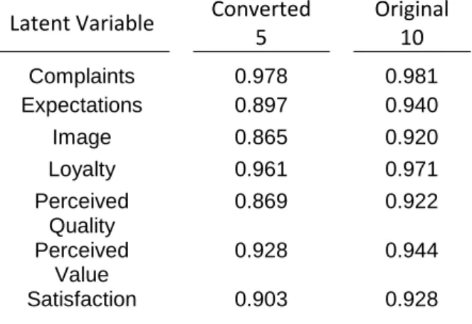
Internal consistency is a test that indicates whether the composites of one latent variable are consistent with each other. It is also called composite reliability. The measurement is in each latent variable, and the value must be higher than 0.7, otherwise the indicators will lack correlation, however, values larger than 0.95 may indicate redundancy of an indicator.

In this study, both the converted 5-length scale and the 10-length scale have internal consistency, and it is higher in the ten-length scale.

However, in both cases the same two latent variables, Loyalty and Complaints, tested for very high composite reliability, as seen in Table 3.4. Both of these constructs have two indicators; in this case, it would be interesting to do the analysis without the indicators that have smaller outer loadings in each of the constructs, if the internal consistency is still good, the analysis with less indicators is better.

Latent Variable Converted 5 Original 10 Complaints 0.978 0.981 Expectations 0.897 0.940 Image 0.865 0.920 Loyalty 0.961 0.971 Perceived Quality 0.869 0.922 Perceived Value 0.928 0.944 Satisfaction 0.903 0.928

Table 3.5 – Composite Reliability

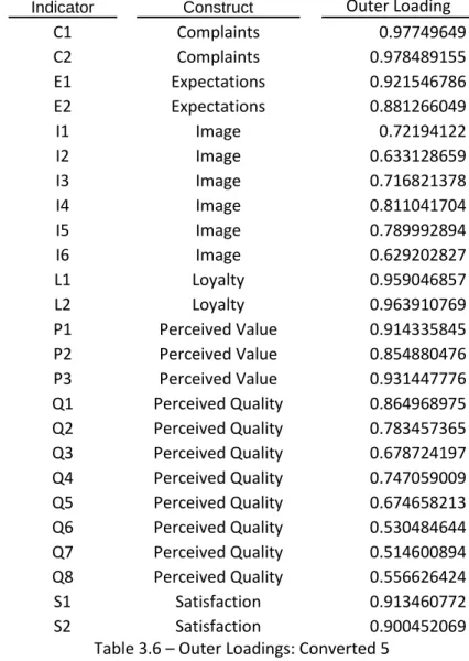
A latent variable should explain a substantial part of each indicator's variance, usually at least 50%. This also implies that the variance shared between the construct and its indicator is larger than the measurement error variance. This means that an indicator's outer loading should be above 0.708 since that number squared (0.7082) equals 0.50. Note that, in most instances, 0.70 is considered close enough to 0.708, thus accepted. Generally, indicators with outer loadings between 0.40 and 0.70 should be considered for removal from the scale only when deleting the indicator leads to an increase in the composite reliability.

As seen in Tables 3.5 and 3.6, the indicators of the converted 5-length scale have a poorer relationship with the latent variables than the indicators of the original 10-length scale. The first one

(20)

14 has 7 indicators with an outer loading smaller than 0.7, making the second scale, 10-length, preferable in this context.

However, from the Table 3.6, we also observe that the indicators Q6 and Q8 in the 10-length should be considered for removal, only if this increases the test of internal consistency.

Indicator Construct Outer Loading

C1 Complaints 0.97749649 C2 Complaints 0.978489155 E1 Expectations 0.921546786 E2 Expectations 0.881266049 I1 Image 0.72194122 I2 Image 0.633128659 I3 Image 0.716821378 I4 Image 0.811041704 I5 Image 0.789992894 I6 Image 0.629202827 L1 Loyalty 0.959046857 L2 Loyalty 0.963910769 P1 Perceived Value 0.914335845 P2 Perceived Value 0.854880476 P3 Perceived Value 0.931447776 Q1 Perceived Quality 0.864968975 Q2 Perceived Quality 0.783457365 Q3 Perceived Quality 0.678724197 Q4 Perceived Quality 0.747059009 Q5 Perceived Quality 0.674658213 Q6 Perceived Quality 0.530484644 Q7 Perceived Quality 0.514600894 Q8 Perceived Quality 0.556626424 S1 Satisfaction 0.913460772 S2 Satisfaction 0.900452069

Table 3.6 – Outer Loadings: Converted 5

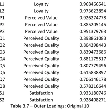
Indicator Construct Outer Loading

C1 Complaints 0.982279058 C2 Complaints 0.980469592 E1 Expectations 0.944946187 E2 Expectations 0.938162699 I1 Image 0.831026231 I2 Image 0.818780217 I3 Image 0.753145946 I4 Image 0.876468192 I5 Image 0.853886252 I6 Image 0.725630996

(21)

15 L1 Loyalty 0.968466541 L2 Loyalty 0.973623854 P1 Perceived Value 0.926274778 P2 Perceived Value 0.885205145 P3 Perceived Value 0.951379763 Q1 Perceived Quality 0.898861083 Q2 Perceived Quality 0.804398443 Q3 Perceived Quality 0.839473686 Q4 Perceived Quality 0.881175517 Q5 Perceived Quality 0.807779496 Q6 Perceived Quality 0.615838897 Q7 Perceived Quality 0.706146178 Q8 Perceived Quality 0.578216644 S1 Satisfaction 0.933180746 S2 Satisfaction 0.928408271

Table 3.7 – Outer Loadings: Original 10

Convergent Validity

Average Variance Extracted (AVE), or Convergent Validity, is defined as the grand mean value of the squared loadings of the indicators associated with the construct (i.e., the sum of the squared loadings divided by the number of indicators). Using the same logic as applied for the individual indicators, an AVE value of 0.50 or higher indicates that, on average, the construct explains more than half of the variance of its indicators. Conversely, an AVE of less than 0.50 indicates that, on average, more error remains in the items than the variance explained by the construct.

In this study, since the majority of the outer loadings of the five-length converted scale are less than 0.70, this makes it a worse option. Also, the AVE confirms the poor explanation of its indicators by the latent variable Perceived Quality, as seen in Table 3.7.

The ten-length original scale has less poor loadings on the Perceived Quality Construct indicators; this explains why the AVE of this construct is higher than in the five-length scale.

Latent Variable Converted 5 Original 10 Complaints 0.956 0.963 Expectations 0.813 0.887 Image 0.519 0.659 Loyalty 0.924 0.943 Perceived Quality 0.461 0.600 Perceived Value 0.811 0.849 Satisfaction 0.823 0.866

(22)

16 Discriminant Validity

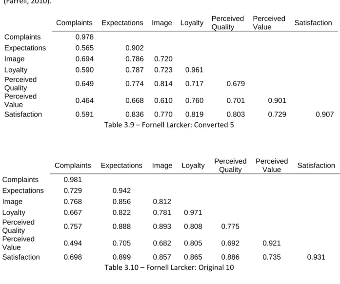
Establishing discriminant validity implies that a construct is unique and captures phenomena not represented by other constructs in the model. Indicator’s outer loading on the associated construct should be greater than all of its loadings on other constructs (cross loadings). According to Fornell-Larcker criterion (Fornell & Fornell-Larcker, 1981): the square root of each constructs’ AVE should be greater than its highest correlation with any other construct. Fornell-Larcker criterion is based on the idea that a construct shares more variance with its associated indicators than with any other construct. Although it seems that the ten-length performs better in this test, in both studies the Image and the Perceived Quality construct do not satisfy the requisite of the discriminant validity, which implies that the two constructs, which are conceptually different, are not sufficiently different in terms of their empirical standards, as shown in Tables 3.8 and 3.9. Thus, in this case, discriminant validity is not established.

The construct Image seems to have fewer issues than the Perceived Quality, which already had issues in previous evaluations. Some items that are measuring Perceived Quality have poor relationship with the construct and, as previous evaluations suggested, running the analysis without a couple (the ones with lowest outer loading) could yield a more satisfactory result in the discriminant validity test (Farrell, 2010).

Complaints Expectations Image Loyalty Perceived Quality Perceived Value Satisfaction Complaints 0.978 Expectations 0.565 0.902 Image 0.694 0.786 0.720 Loyalty 0.590 0.787 0.723 0.961 Perceived Quality 0.649 0.774 0.814 0.717 0.679 Perceived Value 0.464 0.668 0.610 0.760 0.701 0.901 Satisfaction 0.591 0.836 0.770 0.819 0.803 0.729 0.907

Table 3.9 – Fornell Larcker: Converted 5

Complaints Expectations Image Loyalty Perceived Quality Perceived Value Satisfaction Complaints 0.981 Expectations 0.729 0.942 Image 0.768 0.856 0.812 Loyalty 0.667 0.822 0.781 0.971 Perceived Quality 0.757 0.888 0.893 0.808 0.775 Perceived Value 0.494 0.705 0.682 0.805 0.692 0.921 Satisfaction 0.698 0.899 0.857 0.865 0.886 0.735 0.931

(23)

17

3.3.2. Structural Model

Collinearity Assessment

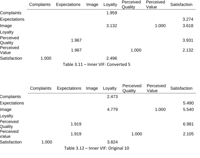
Collinearity boosts standard error, and reduces the ability of rejecting the null hypothesis (path coefficients are significantly not different than zero), especially with PLS-SEM that uses smaller samples (more standard error due to sampling error). It also results in erroneous estimation of the path coefficients, as well as the signs of the effect. To assess the collinearity, we calculate tolerance or Variance Inflation Factor (VIF).

VIF should be lower than 5. If there are collinearity issues, one should treat them, by eliminating constructs, merging into one or creating a high order (dividing constructs).

In this study, it is possible to verify that the model from the ten-length scale has collinearity issues in comparison with the model derived from the five-length converted scale. This may be due to the fact that the sample of the longer scale is smaller in number of respondents than the sample of the shorter converted scale. In Tables 3.10 and 3.11 the inner VIF is shown for the five-length converted scale and original ten-length scale studies.

Complaints Expectations Image Loyalty Perceived Quality Perceived Value Satisfaction Complaints 1.959 Expectations 3.274 Image 3.132 1.000 3.618 Loyalty Perceived Quality 1.967 3.931 Perceived Value 1.967 1.000 2.132 Satisfaction 1.000 2.496

Table 3.11 – Inner VIF: Converted 5

(24)

18 Path Coefficients

The path coefficients represent the estimated change in the endogenous construct for a unit change in the exogenous construct. The goal of PLS-SEM is to identify not only significant path coefficients in the structural model but significant and relevant effects.

With this purpose, Tables 3.12 and 3.13 presents the path coefficients for the converted 5-length scale and the original 10-length scale studies. In turn, Tables 3.14 and 3.15 shows the results for Total Effects to the converted 5-length scale and the original 10-length scale studies.

To test the significance of path coefficients, one should use the bootstrapping procedure: subsamples are randomly drawn (with replacement) from the original set of data. Each subsample is then used to estimate the model. This process is repeated until a large number of random subsamples have been created. The path coefficients estimated from the subsamples are used to derive standard errors for the estimates. With this information, t values are calculated to assess each path coefficient's significance.

Table 3.17 shows the P values for the significance of the path coefficients. At a 90% level of significance, all the coefficients in the converted 5 scale are significant, but in the original 10, two coefficients have failed the test: Complaints  Loyalty and Image  Loyalty.

This could be due to the considerable smaller sample that the longer scale has, or to a poor measuring of the constructs Loyalty, Image and Complaints.

When we first analyzed the skewness and kurtosis, we saw that I1 performed non-normally, and this variable should be considered for removal on a second run of the model. The Image construct also failed in the discriminant validity test, the cross loading with the Expectations construct was higher than the indicator’s outer loading.

After, when analyzing reliability, Loyalty and Complaints indicated some redundancy of indicators, and were higher on the longer scale. And when assessing colinearity in the Structural model, this scale has also failed, but one of the reasons for this was the previously mentioned smaller sample.

Complaints Expectations Loyalty Perceived Quality Perceived Value Satisfaction Complaints 0.100 Expectations 0.417 Image 0.168 0.610 0.127 Loyalty Perceived Quality 0.602 0.226 Perceived Value 0.246 0.701 0.215 Satisfaction 0.591 0.630

(25)

19

Complaints Expectations Loyalty Perceived Quality Perceived Value Satisfaction Complaints 0.094 Expectations 0.424 Image 0.087 0.682 0.148 Loyalty Perceived Quality 0.768 0.279 Perceived Value 0.173 0.692 0.141 Satisfaction 0.698 0.725

Table 3.14 – Path Coefficients: Original 10

Complaints Expectations Loyalty Perceived Quality Perceived Value Satisfaction Complaints 0.100 Expectations 0.247 0.287 0.417 Image 0.310 0.408 0.530 0.428 0.610 0.525 Loyalty Perceived Quality 0.282 0.602 0.329 0.477 Perceived Value 0.385 0.668 0.449 0.701 0.652 Satisfaction 0.591 0.689

Table 3.15 – Total Effects: Converted 5

Complaints Expectations Image Loyalty Perceived Quality Perceived Value Satisfaction Complaints 0.094 Expectations 0.296 0.335 0.424 Image 0.405 0.481 0.546 0.472 0.682 0.580 Loyalty Perceived Quality 0.422 0.768 0.478 0.605 Perceived Value 0.442 0.705 0.501 0.692 0.634 Satisfaction 0.698 0.791

Table 3.16 – Total Effects: Original 10

Converted 5 Original 10

Complaints_ -> Loyalty 4.4% 14.8%

Expectations -> Satisfaction 0.0% 0.0%

Image -> Loyalty 0.3% 38.5%

Image -> Perceived Value 0.0% 0.0%

Image -> Satisfaction 1.7% 5.9%

Perceived Quality -> Expectations 0.0% 0.0% Perceived Quality -> Satisfaction 0.3% 0.0%

Perceived Value -> Expectations 0.0% 0.3%

(26)

20

Perceived Value -> Satisfaction 0.0% 0.5%

Satisfaction_ -> Complaints 0.0% 0.0%

Satisfaction_ -> Loyalty 0.0% 0.0%

Table 3.17 – P values: Path Coefficients

R square and Adjusted R square

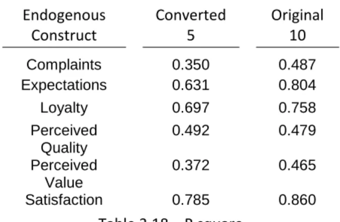
The coefficient of determination R square represents the amount of variance in the endogenous constructs explained by all of the exogenous constructs linked to it. R square values of 0.75, 0.50, or 0.25 for endogenous latent variables can, as a rough rule of thumb, be respectively described as substantial, moderate, or weak. However, researchers want models that are good at explaining the data (thus, with high R square values) with fewer exogenous constructs. Such models are called parsimonious.

Also, the Adjusted R square has to be considered, since R square will always increase when a construct is added to the model, as the Adjusted R square considers in its formula the number of constructs.

In this study, the Adjusted R square is more indicated, since we are comparing models with different number of observations. Tables 3.16 and 3.17 show the results for the R square and adjusted R square for the converted 5-length scale study and the original 10-length scale.

All constructs, except Perceived Quality, are more explained by the exogenous constructs in the ten-length scale than in the five-ten-length, which means that the longer scale is better. In the ten-ten-length, Perceived Quality has to be addressed, again, by comparing the results with the ones of an analysis without some indicators.

Endogenous Construct Converted 5 Original 10 Complaints 0.350 0.487 Expectations 0.631 0.804 Loyalty 0.697 0.758 Perceived Quality 0.492 0.479 Perceived Value 0.372 0.465 Satisfaction 0.785 0.860 Table 3.18 – R square

(27)

21 Endogenous Construct Converted 5 Original 10 Complaints 0.347 0.485 Expectations 0.628 0.802 Loyalty 0.694 0.755 Perceived Quality 0.490 0.476 Perceived Value 0.370 0.462 Satisfaction 0.782 0.857

Table 3.19 – Adjusted R square

f square

In addition to evaluating the R square values of all endogenous constructs, the change in the R square value caused by the omission of a specified exogenous construct from the model can be used to evaluate whether the omitted construct has a substantive impact on the endogenous constructs. Where R square included and R square excluded are the R square values of the endogenous latent variable when a selected exogenous latent variable is included in or excluded from the model. The formula for the f square is:

f square = (R square included – R square excluded)/(1-R square included),

whose values of 0.02, 0.15, and 0.35 (Cohen, 1988), respectively, represent small, medium, and large effects. This study also shows that the effect size relates to the R square of the model, so, if the longer scale has a larger R square, than its effects will also be larger than the smaller scale.

Tables 3.18 and 3.19 shows the f square results for the converted 5-length scale and the original 10-length scale study.

(28)

22

(29)

23

4. CONCLUSION

In light of this analysis, the option for a five points length scale or a ten points length scale is still not clear. At first, the longer scale had a significant lower number of respondents. What we gain in better estimation with the longer scale, the finer intervals demand more time to choose.

Although it has a higher skewness, the ten-length scale has performed better in almost all tests. It has a higher internal consistency, which means that its composites are more correlated in each of the survey’s variable. The longer scale has higher outer loadings and, consequently, higher variance explained by the composites when compared to the smaller scale. It also has more variance explained by the exogenous constructs on the endogenous ones. With ten points, we can observe higher discriminant validity when compared to the smaller scale. The only two tests the ten-length performed worse than the smaller scale was on the VIF and on the significance of the Path

Coefficients, but this is due to having a smaller sample than the shorter survey.

Three variables have performed in a non-normal way since the descriptive observations until the very last tests. I1, Q6 and Q8 were very highly skewed and had excessive kurtosis, because of this, the constructs they were measuring had trouble in the model evaluation. Q6 and Q8 are considerable for removal since they did not present indicator reliability, but only if the results of this removal

increases the AVE of the construct Perceived Quality. Neither the Image or Perceived Quality

construct had discriminant validity, there is a possibility that this would be present if the analysis was re-run without the three non-normal variables.

Due to the nature of the company, one could think that the shorter scale, quicker to answer, would perform better, but the ten-length scale is still a better option for assessing customer satisfaction. However, the market researcher must be aware of the limitations of this scale, since it will yield fewer respondents and the assessment of the results may be impaired by this.

(30)

24

Test Converted

5 Original 10

Respondents Higher Lower

Mean Lower Higher

Skewness Lower Higher

Kurtosis Lower Higher

Composite Reliability Lower Higher

Loading Reliability Lower Higher

Convergent Validity (AVE) Lower Higher

Discriminant Validity (Fornell-Larcker) Not

Established Not Established

Collinearity (VIF) Lower Higher

Precision of Path Coefficients

(Bootstrapping) Higher Lower

Adjusted R² Lower Higher

f² Lower Higher

(31)

25

5. FINAL CONSIDERATIONS

The PLS SEM bias has to be considered: structural model relationships are generally underestimated and measurement model relationships are generally overestimated.

This study only compared one format of scale, with numbers and verbally anchored on the extremes, it would be interesting to compare the ten-length scale used here with one that had verbal

description in all the points, this could yield more respondents than the 201 of this study. What could also yield more responses would be if the scale was 7 points, however, since this study aimed to compare with the ECSI approach, I opted for the 10 point scale.

If the survey was valid for a longer period than the thirteen days it was available and if an email with a reminder to complete the survey was sent after a 10 days of the first email, the ten length scale could have had more respondents and the model would be better.

Other particularity of this study is that it was done online, I do not reject that the results could be different if done using a different data collection method, but I question the advantage of other types of interview due to the online nature of the company and the relationship with the clients maintained through online communication.

(32)

26

6. BIBLIOGRAPHY

Coelho, P. S., & Esteves, S. P. (2007). The choice between a five-point and a ten-point scale in the framework of customer satisfaction measurement. International Journal of Market Research,

49(3), 313–340. Retrieved from

http://apps.isiknowledge.com.ezproxy.leidenuniv.nl:2048/full_record.do?&colname=WOS&sea rch_mode=CitingArticles&qid=3&page=1&product=UA&SID=N2GHKB752fODHdA7Fc2&doc=3 COELHO, P. S., & VILARES, M. J. (n.d.). SATISFAÇÃO E LEALDADE DO CLIENTE: METODOLOGIAS DE

AVALIAÇÃO, GESTÃO E ANÁLISE. ESCOLAR. Retrieved from

https://books.google.pt/books?id=uTRHvgAACAAJ

Cohen, J. (1988). Statistical power analysis for the behavioral sciences. Lawrence Earlbaum

Associates. https://doi.org/10.1234/12345678

Dawes, J. (2008). Do data characteristics change according to the number of scale points used? An experiment using 5-point, 7-point and 10-point scales. International Journal of Market

Research, 50(1), 61–77. https://doi.org/Article

Deng, W. J., Yeh, M. L., & Sung, M. L. (2013). A customer satisfaction index model for international tourist hotels: Integrating consumption emotions into the American customer satisfaction index. International Journal of Hospitality Management, 35, 133–140.

https://doi.org/10.1016/j.ijhm.2013.05.010

Eutsler, J., & Lang, B. (2015). Rating scales in accounting research: The impact of scale points and labels. Behavioral Research in Accounting, 27(2), 35–51. https://doi.org/10.2308/bria-51219 Farrell, A. M. (2010). Insufficient discriminant validity. Journal of Business Research, 63(3), 324–327.

https://doi.org/10.1016/j.jbusres.2009.05.003

Fornell, C., & Larcker, D. F. (1981). Evaluating Structural Equation Models with Unobservable Variables and Measurment Error. Journal of Marketing, 18(1), 39–50.

https://doi.org/10.2307/3151312

Friedman, H. H., & Amoo, T. (1999). Rating The Rating Scales. The Journal of Marketing Management. https://doi.org/10.2307/3151463

Gunter, B., Nicholas, D., Huntington, P., & Williams, P. (2002). Online versus offline research: Implications for evaluating digital media. Aslib Proceedings.

https://doi.org/10.1108/00012530210443339

Hicks, C. L., Von Baeyer, C. L., Spafford, P. A., Van Korlaar, I., & Goodenough, B. (2001). The Faces Pain Scale - Revised: Toward a common metric in pediatric pain measurement. Pain. https://doi.org/10.1016/S0304-3959(01)00314-1

Hjermstad, M. J., Fayers, P. M., Haugen, D. F., Caraceni, A., Hanks, G. W., Loge, J. H., … Kaasa, S. (2011). Studies comparing numerical rating scales, verbal rating scales, and visual analogue scales for assessment of pain intensity in adults: A systematic literature review. Journal of Pain

and Symptom Management. https://doi.org/10.1016/j.jpainsymman.2010.08.016

Hsu, S. H. (2008). Developing an index for online customer satisfaction: Adaptation of American Customer Satisfaction Index. Expert Systems with Applications.

(33)

27 Ilieva, J., Baron, S., & Healey, N. M. (2002). Online surveys in marketing research: pros and cons |

Nigel Healey and Janet Ilieva - Academia.edu. International Journal of Market Research. Lee, E. Y., & Park, C. S. (2015). Does advertising exposure prior to customer satisfaction survey

enhance customer satisfaction ratings? Marketing Letters, 26(4), 513–523. https://doi.org/10.1007/s11002-014-9285-2

Ngo, V. M., & Nguyen, H. H. (2016). The Relationship between Service Quality, Customer Satisfaction and Customer Loyalty: An Investigation in Vietnamese Retail Banking Sector. Journal of

Competitivenes, 8(2), 103–116. https://doi.org/10.7441/joc.2016.02.08

Peterson, R. A., & Wilson, W. R. (1992). Measuring customer satisfaction: Fact and artifact. Journal of

the Academy of Marketing Science, 20(1), 61–71. https://doi.org/10.1007/bf02723476

Ringle, C., Wende, S., & Becker, J. (2015). SmartPLS 3.2.4. Retrieved From. https://doi.org/http://www.smartpls.com