Random Environments
Patr´ıcia A. Filipe
1and Carlos A. Braumann
11 Universidade de ´Evora, Centro de Investiga¸c˜ao em Matem´atica e Aplica¸c˜oes
Rua Rom˜ao Ramalho, 59, 7000-671 ´Evora, Portugal [email protected], [email protected]
Abstract: We have considered, as general models for the evolution of animal size in a random environment, stochastic differential equations of the form dY (t) =
b (A − Y (t)) dt + σdW (t), where Y (t) = g(X(t)), X(t) is the size of an animal at
time t, g is a strictly increasing function, A = g(a) where a is the asymptotic size,
σ measures the effect of random environmental fluctuations on growth, and Wt
is the Wiener process. We have considered the stochastic Bertalanffy-Richards model (g(x) = xc with c > 0) and the stochastic Gompertz model (g(x) =
ln x). We have studied the problems of parameter estimation for one path and also considered the extension to several paths. We also used bootstrap methods. Results and methods are illustrated using bovine growth data.
Keywords: growth models; stochastic differential equations; estimation; cattle weight.
1
Introduction
The most common models used to describe the growth of an individual animal in terms of its size X(t) at time t have assumed the form of a differential equation dY (t) = b(A − Y (t))dt, Y (t0) = y0, where we made a change of variable Y (t) = g(X(t)) with g a strictly increasing function (which we assume known). We have y0 = g(x0) and A = g(a), where x0 is the size at birth and a is the asymptotic size or size at maturity of the animal. The parameter b > 0 is a rate of approach to maturity.
The Bertanlanffy-Richards model (Bertalanffy (1957) and Richards (1959)) corresponds to the choice g(x) = xc for c > 0 (typical choices are c = 1
and c = 1/3) and the Gompertz model corresponds to g(x) = ln x (can be considered the limiting case of Bertalanffy-Richards model when c → 0). If the animal is growing in a randomly fluctuating environment, we can model growth through a stochastic differential equation (SDE) of the form
dY (t) = b (A − Y (t)) dt + σdW (t), (1) where σ > 0 measures the strength of environmental fluctuations and W (t) is a standard Wiener process. Garcia (1983) applied these type of models to tree growth.
The solution of (1) is a homogeneous diffusion process with drift and diffu-sion coefficient, respectively, b(A − y) and σ2. The solution of this SDE is Y (t) = A + e−bt(y
0− A) + σe−bt Rt
0ebsdW (s) (see, for instance, Braumann (2005)). The distribution of Y (t) is Gaussian with mean A + e−bt(y
0− A) and variance σ2
2b(1 − e−2bt) and converges, as t → +∞, to a Gaussian dis-tribution with mean A and variance σ2
2b.
The data used for illustration is the weight of ”mertolengo” cattle of the ”rosilho” strand and was provided by Carlos Roquete (ICAM-UE).
2
Parameter estimation
In Filipe et al. (2007), we have considered, for a single path, the statistical problems of parameter estimation and of prediction of future sizes of an animal for model (1). Subsection 2.1 gives a brief summary of the estimation part. Subsection 2.2 presents the extension of the estimation methods to the case of several paths, assumed to be independent. We have also studied bootstrap estimation methods, shown on subsection 2.3.
2.1 Parameter estimation for a single path
Let us assume we observe the evolution of the weight of one animal at times 0 = t0 < t1 < ... < tn, and represent the weight of the animal at time tk
(k = 1, 2, ..., n) by Xk = X(tk). Let Yk = g(Xk) and Y = (Y0, Y1, ..., Yn). We want to estimate p = (A, b, σ). Since we know the transition distribu-tions of Y (t), using the fact that it is a Markov process and given Y0= y0, assumed known, we can obtain the log-likelihood function
LY(p) = −n 2ln µ 2πσ2 2b ¶ −1 2 n X k=1 ln¡1 − Ek2 ¢ − b σ2 n X k=1 (yk− A − (yk−1− A) Ek)2 1 − E2 k ,
with Ek = e−b(tk−tk−1). In terms of X the log-likelihood function is LX(p) = LY(p) + Pn k=1ln ³ dY dX ¯ ¯ x=xk ´
. The maximum likelihood estimator (MLE), ˆ
p, is obtained by maximization of LY (equivalent to maximization of LX). Using the properties of MLE and Y (t) we can obtain the Fisher information matrix and construct approximate confidence intervals for the parameters. In Filipe et al. (2007), we used data of the weight in kg of a single animal for which we had 79 observations. We have applied model (1) for the particular cases g(x) = xc (c > 0) and g(x) = ln x (c = 0) (Table 1). Some choices of c were considered and the models which turned out to be the best choices
TABLE 1. Maximum likelihood estimates, log-likelihood value and approximate 95% confidence intervals (data from one animal).
a b σ LX
c = 0(Gompertz) 407.1 ± 60.5 1.472 ± 0.354 0.226 ± 0.036 −338.12 c = 1/3 422.4 ± 81.6 1.096 ± 0.525 0.525 ± 0.083 −337.88
2.2 Parameter estimation for several paths
Assume we have data on m animals. The weight of animal number j (j = 1, 2, ..., m) is observed at times 0 = tj,0 < tj,1 < ... < tj,nj, and is, respectively, Xj,0 = X(tj,0), Xj,1 = X(tj,1), ... , Xj,nj = X(tj,nj). Let Yj,k = Y (tj,k) = g(Xj,k) (j = 1, 2, ..., m; k = 1, 2, ..., nj) and Yj = ¡
Yj,0, Yj,1, ..., Yj,nj ¢
.
For animal number j we can obtain the log-likelihood LYjby proceeding as in the case of a single path. From independence, the overall log-likelihood for the m animals is LY1,Y2,...,Ym(p) =
Pm
j=1LYj(p). The MLE ˆp is ob-tained, now, by maximization of LY1,Y2,...,Ym.
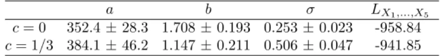
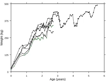
In Filipe and Braumann (2007), we have applied the procedure for the stochastic Bertalanffy-Richards model, for the cases c = 0 and c = 1/3, to the data of m = 5 animals of the same strand raised under similar condi-tions. In Figure 1 we can see the observed weights for these 5 animals. For one animal we have 79 observations and the other four have 38 observations each. Table 2 shows the results obtained.
TABLE 2. Maximum likelihood estimates, log-likelihood value and approximate 95% confidence intervals (data from 5 animals).
a b σ LX1,...,X5
c = 0 352.4 ± 28.3 1.708 ± 0.193 0.253 ± 0.023 -958.84
c = 1/3 384.1 ± 46.2 1.147 ± 0.211 0.506 ± 0.047 -941.85
2.3 Bootstrap methods
The asymptotic confidence intervals obtained from the Fisher information matrix may be quite unreliable for small sample sizes. In such case, boot-strap methods are recommended.
In Efron and Tibshirani (1993) we can find two types of bootstrap proce-dure, respectively, parametric bootstrap (PB) and nonparametric bootstrap (NPB). We have applied these two bootstrap methods for the cases c = 0 and c = 1/3.
0 1 2 3 4 5 6 Age (years) 0 125 250 375 500 Weight (kg)
FIGURE 1. Observed growth curves for the 5 animals.
For PB, we have considered the Gaussian distribution of Yk, mentioned
on section 1, and, using the MLE ˆp to approximate p, generated 1000 independent "samples", y∗i = ¡y∗i
0 , y1∗i, ..., y∗in
¢
(i = 1, ..., 1000). For each one of these "samples" we have computed the estimates ˆp∗i(i = 1, ..., 1000)
(following the procedure described in subsection 2.1), and consequently, by calculating the mean, obtained the bootstrap estimate ˆp∗.
Extending this procedure to m animals, we have generated y∗i
j = (y∗ij,0, y∗ij,1, ..., y∗i
j,nj) (i = 1, ..., 1000; j = 1, ..., m) using as an approximation of p the overall MLE, ˆp, presented in subsection 2.2. We have obtained, for each
i = 1, ..., 1000, the maximum likelihood estimates ˆp∗i as in subsection 2.2.
From the 1000 replicates ˆp∗i(i = 1, ..., 1000), to obtain ˆp∗ the procedure is
similar to the one presented for a single animal.
For the NPB method we can find in Efron and Tibshirani (1993) how to approach the problem of dependency between observations, wich must be considered in our case. We can see that
ek=¡etkYk− etk−1Yk−1− A¡etk− etk−1¢¢± r
σ2(e2tk− e2tk−1)
2b , (2)
for k = 1, ..., n, are i.i.d with standard Gaussian distribution. We have ob-tained 1000 independent replicates, e∗i=¡e∗i
0, e∗i1, ..., e∗in
¢
(i = 1, ..., 1000) where the e∗i
replacement the empirical distribution of the observed values of e1, ..., en. For each i=1,..., 1000, we have used e∗i to reconstruct, using the inverted
expression of (2), a vector of n observations y∗i. We can, then, obtain the
bootstrap estimates of the parameters in the same way as in PB.
In case we have m animals, in a similar way we must consider ejk, i.i.d
with standard Gaussian distribution. For each path we proceed as described above for a single animal.
For both PB and NPB, the standard bootstrap confidence intervals are obtained using normality and the sample standard deviation of the 1000 replicates of the estimates. We can also obtain bootstrap confidence inter-vals using the empirical quantiles, which, in our example, gives very similar results.
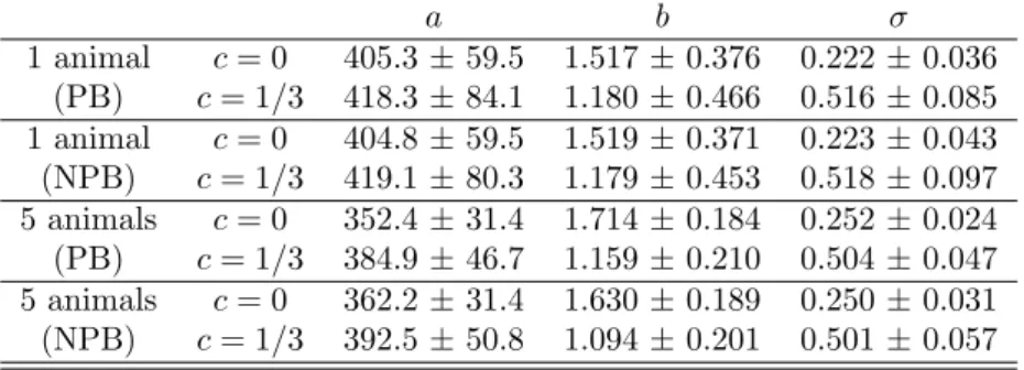
Although our data has a reasonably large sample size, for illustration pur-poses we still obtained the bootstrap estimates and 95% confidence intervals for both PB and NPB (see Table 3).
TABLE 3. Bootstrap estimates and 95% confidence intervals
a b σ 1 animal c = 0 405.3 ± 59.5 1.517 ± 0.376 0.222 ± 0.036 (PB) c = 1/3 418.3 ± 84.1 1.180 ± 0.466 0.516 ± 0.085 1 animal c = 0 404.8 ± 59.5 1.519 ± 0.371 0.223 ± 0.043 (NPB) c = 1/3 419.1 ± 80.3 1.179 ± 0.453 0.518 ± 0.097 5 animals c = 0 352.4 ± 31.4 1.714 ± 0.184 0.252 ± 0.024 (PB) c = 1/3 384.9 ± 46.7 1.159 ± 0.210 0.504 ± 0.047 5 animals c = 0 362.2 ± 31.4 1.630 ± 0.189 0.250 ± 0.031 (NPB) c = 1/3 392.5 ± 50.8 1.094 ± 0.201 0.501 ± 0.057
3
Conclusions
Stochastic differential equations models for the growth of individual ani-mals where considered and parameter estimation were developed for the case of several animals. In progress is the study of nonparametric estima-tion of the drift and diffusion coefficients, with the goal of finding a more general growth model. We have also considered the more realistic case in which we have different asymptotic expected size for different animals (to appear).
Acknowledgments: Both authors are members of CIMA, research cen-ter financed by FCT (Funda¸c˜ao para a Ciˆencia e a Tecnologia) within its ’Programa de Financiamento Plurianual’. This work was financed by FCT within the research project PTDC/MAT/64297/2006.
References
Bertalanffy, L. von. (1957). Quantitative laws in metabolism and growth.
The Quarterly Review of Biology, 34, 786-795.
Braumann, C. A. (2005). Introdu¸c˜ao ´as Equa¸c˜oes Diferenciais Estoc´asticas. Edi¸c˜oes SPE.
Efron, B. and Tibshirani, R. J. (1993). An Introduction to the Bootstrap. Chapman & Hall.
Garcia, O. (1983). A stochastic differential equation model for the height of forest stands Biometrics, 39, 1059-1072.
Filipe, P. A. and Braumann C. A. (2007). Animal growth in random envi-ronments: estimation with several paths. Bulletin of the International
Statistical Institute, vol. LXII (in press).
Filipe, P. A., Braumann C. A. and Roquete, C. J. (2007). Modelos de cresci-mento de animais em ambiente aleat´orio. In: Estat´ıstica Ciˆencia
In-terdisciplinar, Actas do XIV Congresso Anual da Sociedade Por-tuguesa de Estat´ıstica. 401-410, Edi¸c˜oes SPE.
Richards, F. (1959). A flexible growth function for empirical use. Journal