Development of a Variable Geometry Ejector for a Solar Desalination System

(1)

Diogo Nunes Couto e Sá

A Thesis in the Field of Energy Management

for the Degree of Master of Science in Mechanical Engineering

Advisor: Dr. João Soares

Co-Advisor: Dr. Szabolcs Varga

June 2019

Development of a Variable Geometry

Ejector for a Solar Desalination System

(2)

ii

(3)

iii

Abstract

There is a scarcity of fresh-water resources that with the growing of the world's population require sustainable solutions for the use of the planet’s water resources. Solar desalination is one of the solutions. Multi-effect Desalination using a Thermo Vapor Compressor (MED-TVC) presents the least energy intensive method of desalination.

MED-TVC have ejectors as key system components, which permit to attain high performance at design conditions. However, using renewable energy sources lead to an extended range of operational conditions. Ejector’s efficiency drops significantly when operating at off-design conditions. A solution is to use a variable geometry ejector, i.e. geometry adapts to operation conditions.

Research was performed to optimize the ejector entrainment ratio for various motive flow temperature conditions.

Apart from the having the movable Nozzle eXit Position (NXP) implemented on the first geometry, an ejector geometry with bigger constant area section length and other with half of the diffuser angle were created employing the movable NXP.

FLUENT, commercially available Computational Fluid Dynamics (CFD) software, was used to model every ejector geometry for each proposed motive flow temperature. A conventional finite-volume scheme, using steady-state flow and axis-symmetric conditions, was used to solve two-dimensional transport equations with the realizable k-ε turbulence model. A CFD model was successfully developed for steam ejector design and performance analysis.

The objective of the study was to investigate the optimal NXP for every simulated geometry and that way finding the optimum entrainment ratio (i.e. ejector performance). This study also assessed how changing the ejector's geometry would influence the entrainment ratio as well as the optimum position of the NXP.

The results from the study indicate that the variable geometry ejector efficiency improves compared to a conventional jet-ejector design. However, the improvement is not significant when compared to a compromise NXP position that can be found with statistical calculations. It was found that for a NXP 25 millimeters upstream of its original position, the entrainment ratio values did not differ more than 1.63% from the best entrainment ratio values for each temperature. Moreover, 120ºC motive flow was the temperature with the best entrainment ratio (170.1%).

(4)

(5)

v

Resumo

Existe uma crescente escassez global de água doce, o que associado ao crescimento da população mundial requere novas soluções sustentáveis para o uso do recurso aquífero do planeta. A dessalinização com recurso a energia solar é uma das soluções possíveis.

Ejetores permitem atingir uma performance elevada nas condições para que foi projetado. Contudo, as fontes renováveis de energia apresentam um caracter intermitente o que leva a uma gama de condições operacionais alargada. A eficiência dos ejetores decresce significativamente quando operam em condições fora das condições de projeto. Uma solução é o uso de um ejetor de estrutura variável, i.e. a geometria do ejetor adapta-se às condições de operação.

Foi realizado um estudo para a otimização do entrainment ratio de um ejetor para várias temperaturas de entrada do fluido primário. Para além de uma primeira geometria original de um ejetor, foram criadas mais duas geometrias, uma com o comprimento da secção de área constante maior e outra com metade do angulo do difusor. Em todas as geometrias foi implementado um NXP móvel.

FLUENT, um software de licença comercial para simulação de dinâmica dos fluidos computacional (CFD), foi utilizado para modelar todas as geometrias de ejetores sob todas as condições de temperatura propostas. Foi usado um esquema de volumes finitos, em estado estacionário e axi-simétrico para resolver as equações de transporte com um modelo de turbulência realizable k-ε. Um modelo CFD foi desenvolvido com sucesso para o design e análise da performance de ejetores.

O objetivo deste estudo foi investigar a posição ótima do NXP para cada geometria e temperatura simulada de forma a descobrir o melhor entrainment ratio. Outro objetivo passou por estudar de que maneira a mudança de geometria do ejetor afeta o entrainment ratio bem como na posição ótima do NXP.

Os resultados deste trabalho provam que ter um ejetor de geometria variável aumenta a eficiência do mesmo quando comparado com um ejetor de geometria fixa. Este aumento de eficiência, não é porém, significativo quando comparado com uma posição compromisso do NXP que pode ser calculada com meios estatísticos. Para um NXP 25 milímetros a montante da sua posição original, o valor de entrainment ratio não diferiu mais do que 1,63% do melhor valor para cada temperatura. Um fluxo principal de 120ºC foi o que obteve melhores resultados de entrainment ratio (170,1%).

(6)

(7)

vii

Acknowledgements

I would first like to thank my family for providing me with unfailing support and continuous incitement over my student years to overcome myself and to do not leave any goal to be unfulfilled. This is the culmination of the best education I could have asked for. This accomplishment would not have been possible without them.

I would also express my deepest gratitude to my thesis coordinators, Dr. João Soares and Dr. Szabolcs Varga. The doors to their offices were always open whenever I needed. They allowed this thesis to be my own work, but steered me in the right direction at every crucial phase or whenever they saw the need to. Working with them was a great experience, without their knowledge I am sure I would not have done this work with the same confidence and most importantly I would definitely not had learn so much as I did this semester.

I would also like to thank the CIENER's investigators who helped in innumerous stages of this research project: Behzad, Hugo and Vu. Without their participation and knowledge, the number of simulations on this work would have been reduced significantly.

Finally, I must express my very profound gratitude to the amazing group of friends I have in FEUP for such fun times and continuous support throughout our university years. We were all at the same boat and are finally reaching the beach.

To you all, thank you. Diogo.

(8)

(9)

ix

List of Figures

Figure 1.1 - Projected increase in global water stress by 2040 [3]. ... 2

Figure 1.2 – Water use and water resources per capita trends over the years. ... 3

Figure 1.3 - Cost of different methods of alternative water supply [8]... 3

Figure 1.4 - World's annual average direct normal radiation [13]. ... 4

Figure 1.5 – Desalination CO2 emissions in 2016 and 2040 (predicted). ... 5

Figure 1.6 - Global Water Desalination Market Size, 2014-2025 (USB Billion) [18]. ... 6

Figure 1.7 – Annual energy to come from clean sources for desalination Plants. ... 8

Figure 1.8 – Percentage of different desalination plants sizes ... 9

Figure 2.1 - Desalination in a nutshell. ... 11

Figure 2.2 – Percentage of cost distribution for three desalination methods [30]. ...13

Figure 2.3 - Diagram of a multi-effect distillation plant. ... 17

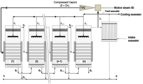
Figure 2.4 - Illustration of MED-TVC system with n effects. ... 18

Figure 2.5 - Ejector schematic design. ... 20

Figure 2.6 - Two typical ejector types: (a) Constant Pressure Mixing ejector and (b) Constant Area Mixing ejector. ...21

Figure 2.7 – Velocity and Pressure changes when the flow faces a convergent or divergent area in supersonic and subsonic flows. ... 22

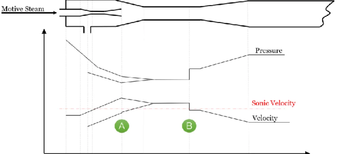
Figure 2.8 – Approximated Pressure and velocity variation inside an ejector. ... 23

Figure 2.9 - Ejector operational mode. ... 24

Figure 2.10 - Effective area in the ejector throat. ... 26

Figure 2.11 - The variation of the entrainment ratio with the primary fluid pressure obtained from CFD simulation [63]. ... 27

Figure 2.12 - Effect of the area ratio on the entrainment ratio and critical back-pressure. ... 29

Figure 2.13 - Typical behaviour of entrainment ratio with the growth of the length of the mixing chamber. ... 30

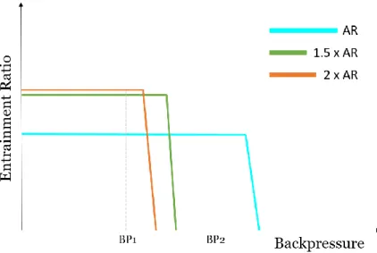
Figure 2.14 - Entrainment ratio and critical backpressure comparison between a fixed geometry and a variable geometry ejector. ... 32

(12)

xii

Figure 2.15 - Structure of an auto-tuning AR ejector [79]. ... 32

Figure 3.1 – Diagram tree of different methods to model a fluid problem ... 35

Figure 3.2 - Blackbox representation. ... 36

Figure 3.3 - Schematic representation of the numerical modeling process. ... 37

Figure 3.4 - A representation of a structured mesh arrangement [90]. ... 39

Figure 3.5 - Representation of a RCM re-order [93]. ... 40

Figure 3.6 - Classification of different pressure–velocity coupling algorithms [98]. ...42

Figure 3.7 – Energy Cascade of Richardson. ...44

Figure 3.8 – Different turbulence models on the energy spectrum. ... 45

Figure 3.9 – Representation of how RANS uses time-averaging of fluctuation components of velocity. ...46

Figure 4.1 - Mesh optimization procedure ... 60

Figure 4.2 – Simulation’s optimization procedure. ... 61

Figure 4.3 - Original mesh geometry. ... 63

Figure 4.4 - Constant area section change geometry. ... 63

Figure 4.5 - Diffuser angle change geometry. ...64

Figure 4.6 - Mesh geometry with pointed boundary conditions... 65

Figure 4.7 - Poorly designed near-wall mesh. ... 65

Figure 4.8 - Quality design near-wall mesh. ...66

Figure 5.1 - Ejector Performance with different NXP for 120ºC. ... 74

Figure 5.2 - Pressure - E.R. plot comparison with two different critical Back-Pressure. ... 75

Figure 5.3 - Ejector Performance with different NXP and back Pressures for 120ºC. ... 76

Figure 5.4 - Mach-Number pathlines of 120ºC with original backpressure; L=40. ... 76

Figure 5.5 - Mach-Number pathlines of 120ºC with new back pressure; L=-25. ... 77

Figure 5.7 - Mach-Number Color-Map of 130ºC with L=0... 78

Figure 5.8 - Mach-Number Color-Map of 130ºC with L=-25. ... 79

(13)

xiii

Figure 5.11 - Mach-Number pathlines of 140ºC with L=-15. ... 80

Figure 5.16 - Diffuser focused Mach-Number pathlines of 150ºC with L=-20. ... 83

Figure 5.17 - Diffuser focused Mach-Number pathlines of 150ºC with L=-35. ... 83

Figure 5.18 - Ejector Performance with different NXP for 160ºC, 170ºC and 180ºC. ... 84

Figure 5.20 - Color-map of the supersonic areas on the diffuser section at a motive flow of 130ºC with L=-20. ... 87

Figure 5.21 - Color-map of the supersonic areas on the diffuser section at a motive flow of 130ºC with L=20. ... 87

Figure 5.22 - Color-map of the supersonic areas on the diffuser section at a motive flow of 140ºC with L=-20. ... 88

Figure 5.23 - Comparison of supersonic flows at the diffuser entrance. ... 94

Figure 5.24 - Optimum NXP for each motive flow temperature. ... 96

Figure 5.25 - Optimum entrainment ratio per motive flow temperature... 98

(14)

(15)

xv

List of Tables

Table 2.1 - Energy required to deliver 1m3_{of water for human consumption from}

various water sources [27]. ...12

Table 2.2 - Membrane vs thermal desalination cost per feed water source and production capacity [7]. ... 14

Table 2.3 - Characteristics of different desalination methods [22, 31-34]. ... 15

Table 2.4 - Driving flow status at the supersonic nozzle exit [60]. ... 25

Table 3.1 - Summary-Table of all the possible turbulence models to use on this project [94, 104, 109, 110]. ... 57

Table 4.1 - Boundary conditions in respect of Figure 4.5. ... 65

Table 4.2 - Mesh independence tests for a motive flow of 130ºC. ... 67

Table 4.3 - Mesh independence tests for a motive flow of 140ºC. ... 68

Table 4.4 - Parameters selected for the model solver. ... 69

Table 4.5 - Parameters selected for the energy equation and turbulence model. ... 70

Table 4.6 - Parameters selected for the boundary conditions. ... 70

Table 4.7 - Parameters selected for the primary inlet. ... 71

Table 4.8 - Parameters selected for fluid characterization. ... 71

Table 4.9 - Discretization parameters selected on Fluent. ... 72

Table 5.1 - Mass flow rate comparison on the optimum geometry for motive flow of 170ºC and 180ºC. ... 84

Table 5.2 - Entrainment ratio results of the simulations on the first geometry. ... 85

Table 5.3 - Recirculation length comparison between the original geometry and geometry 2. ... 89

Table 5.4 - Entrainment ratio results of all the simulations on the second geometry. .. 90

Table 5.5 - Comparison of results between Geometry 1 and 2. ... 91

Table 5.6 - Recirculation length comparison between the original geometry and geometry 3. ... 92

(16)

xvi

Table 5.7 - Comparison of results between Geometry 1 and 3. ... 93

Table 5.8 - Entrainment ratio results of all the simulations on the third geometry. ... 95

Table 5.9 - E.R. improvement with the movable NXP for each temperature. ... 97

(17)

(18)

xviii

Nomenclature

Acronyms (sorted alphabetically)

AR Area Ratio

BC Boundary Condition

CAM Constant Area Mixing

CFD Computational Fluid Dynamics

CM Cuthill–McKee

COP Coefficient of performance CPM Constant Pressure Mixing DNS Direct Numerical Simulation

EDR Electrodialysis Reversal Desalination

ER Entrainment Ratio

GWI Global Water Intelligence

IPCC Intergovernmental Panel on Climate Change

LES Large Eddy Simulation

MED Multi effect evaporation desalination

MED-TVC Multi-effect Desalination using a Thermo Vapour Compressor MENA Middle East and North Africa

MFR Mass Flow Rate

MSF Multistage Flash

NXP Nozzle Exit Position

OECD Organization for Economic Co-operation and Development RANS Reynolds Averaged Navier-Stokes

RCM Reverse Cuthill–McKee

RE Renewable Energy

RO Reverse Osmosis

RSM Reynolds Stress Model

TVC Thermal Vapor-Compression

(19)

xix Greek letters (sorted alphabetically)

∇ Divergence

δ Kronecker delta

ε Rate of dissipation of turbulence energy

μ Dynamic viscosity

ρ Fluid Density

τ Viscous stress

Ω Specific dissipation rate

Parameters (sorted alphabetically)

D Diameter

div Divergence

F Mass force per volume unit

h Total energy

k Turbulent kinetic energy L

P Pressure

R Reynolds stress tensor

Re Reynolds Number

S Strain rate tensor

t Time

v Flow velocity vector x Flow Position vector

Subscripts (sorted alphabetically) i x j y t Time Superscripts ( )̀ Fluctuation value ( ) ̅̅̅̅ Time-averaged value

(20)

(21)

1. Introduction

Water, energy and environmental issues hold hands.

1.1 - World Paradigm

Water plays a vital role in every ecosystem of planet Earth being a fundamental necessity for human lives and livelihoods. Water is needed to drink, to grow food on, to keep environments clean and even to keep populations warm or cold, civilizations that harnessed water thrived and those who didn’t fell.

There is no doubt that water is a key resource of planet Earth, yet populations are not managing this resource well or even making the most of it. In a society where, since birth, people are used to naturally flows water every time a tap is opened anytime that they want, as much as they want, is easy to underestimate the effects of inadequate water management can play out over a lifetime.

At this day, half of the world’s population live in areas where demand for water resources surpasses the supplies of sustainable water sources [1]. About 71% of the Earth’s surface is covered in water, but if all the water could be concentrated into a big sphere, it would be around 1385 km in diameter, nine times shorter than Earth diameter. From the 1.2 trillion cubic meters of water on Earth, 97% of it is salt water and 2% is frozen in the poles or deep in the ground, unavailable to humans [2]. Also, the main aspect of the world’s freshwater resources is that is very unevenly distributed.

The domestic water use (drinking, cooking, bathing and cleaning) however plays only a small part of the total of water that is consumed. The industry uses twice as much water as households specially for cooling and water is needed to produce food and crops irrigating the fields uses nearly 70% of the total withdrawn for human uses [1].

(22)

2

WRI’s Aqueduct Water Stress Projections based on the latest data from the Intergovernmental Panel on Climate Change (IPCC) 5th Assessment Report (AR5) provide estimates of water stress, demand, supply, and seasonal variability for the years 2020, 2030, and 2040. This study shows that in 2040 most of the world will not have enough water to meet demand during all year as shown as in Figure 1.1.

Figure 1.1 - Projected increase in global water stress by 2040 [3].

Day Zero marks the day when a certain city’s taps would not flow more water because its reservoirs would become dangerously low on water. Numerous cities worldwide have experienced water supply crises in recent years. Cities like Barcelona, Melbourne, São Paulo and Beijing are among them [3].

The most extreme case, yet, was in Cape Town were due to climatic causes, high urban population growth and deficient water supply systems led to the verge of a Day Zero that was only avoided thanks to water rationing and a rainy season. Cape Town has since taken measures to avoid a Day Zero in 2019 and afterwards, the city has increased the water management programmes and created restrictions on the water consumption per person [4].

This examples and measures should be taken seriously by other cities and countries, indeed, much water could be saved with real shifts toward low water-wasting types of management.

Sustainable water management should also be considered and manage the separation of water supplies for drinking water, other purposes for domestic use and agricultural use water. In addition, rainwater harvesting, separate collection of wastewater streams, and recycling of water offer better planning options for the future.

(23)

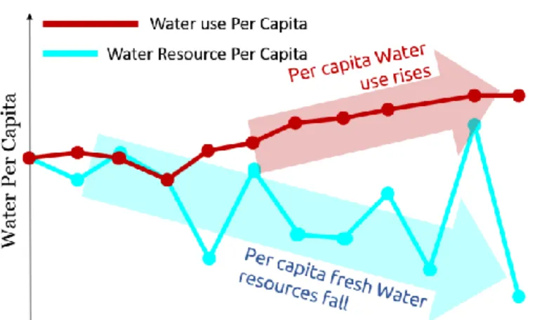
3 As seen in Figure 1.2, in recent years, an important balance of water use and fresh water resources per capita has been broken. The water necessities will continue growing as the world population follows the same path.

Figure 1.2 – Water use and water resources per capita trends over the years.

The only nearly inexhaustible source of water is in the oceans. Yet, high salinity water is not safe for drinking neither for agricultural purposes. Desalination tackles this drawback giving the world population infinite amounts of freshwater, however, it is an energy-intensive process, and thus it comes at a high cost [5, 6]. For example, even the most straightforward desalination technique (single stage evaporation) requires about 650 (kW.ht)/ m3_{. Desalination energy consumption represents about} 30% to 50% of the cost of water produced [7] and is the most energy-intensive fresh water process (see Figure 1.3).

(24)

4

In 2013 the global installed capacity of desalination freshwater was already 80 million m3_{of fresh water a day [9] and in 2017 nearly 93 million m}3_{a day by around} 18,500 desalination plants [10].

Desalination plants in the Middle East and North Africa (MENA) region produce 48% of the world’s desalinated water [11]. These countries rely on desalination water almost as the only freshwater source. Saudi Arabia alone produces more than 5 million cubic meters of desalinated water per day, making it nearly 50% of the country’s water supply.

MENA region have had abundance of energy resources over the years, relying mainly on oil to meet its energy necessities, however, the region has ranges between 2050 and 2800 kWh/m2_{/year of direct normal radiation and cloud cover is rare [12].}

Figure 1.4 - World's annual average direct normal radiation [13].

As technology evolves and the price of crude oil keeps climbing, a shifting towards Renewable Energy (RE) sources is happening in every energy demanding process and desalination is no exception. Solar powered desalination techniques are in vogue in the industry. The technology is mature enough and provides easy installation, operation and maintenance as well as reasonable efficiency. This technology is the ideal technology for water demands less than 50 m3_{/day [14].}

Within two decades, renewable energy sources will be the world’s main energy source of power. Wind, solar and other renewables will account for about 30% of the world’s electricity supplies by 2040 [15].

The purpose of introducing more and more renewable energy into the energy system was to save fuel, with time and studies, companies started to realize that a fossil fuel free reality with all the commodities that the 21st century citizen needs was

(25)

5 possible. As the supply of oil and coal decreases, their prices will increase so as the costs of products and services that depend on them. The solution to prevent an energy crisis would be to increasingly replace and eliminate non-renewable energy source devices and activities for renewable ones.

The CO2 emissions on the last years showed differences on approach on energy policies. On the one hand, the Organization for Economic Co-operation and Development (OECD) countries (all developed countries) had a decrease of 1.4% on CO2 emissions and on the other hand the non-OECD countries (such as China, Russia and India) had a 2.7% increase of CO2 emissions.

For years it was thought that decarbonization and changing the energy sources from oil and gas to renewables was a drawback in economic growth. New studies suggests that not only this is wrong, the shifting to renewable energy sources meant a significant driver in economic growth. In countries like China, Canada, France, Germany, Italy, Kenya, Portugal, Spain and the United Kingdom the renewable energy consumption had a significant positive effect on economic growth in the long-run [16].

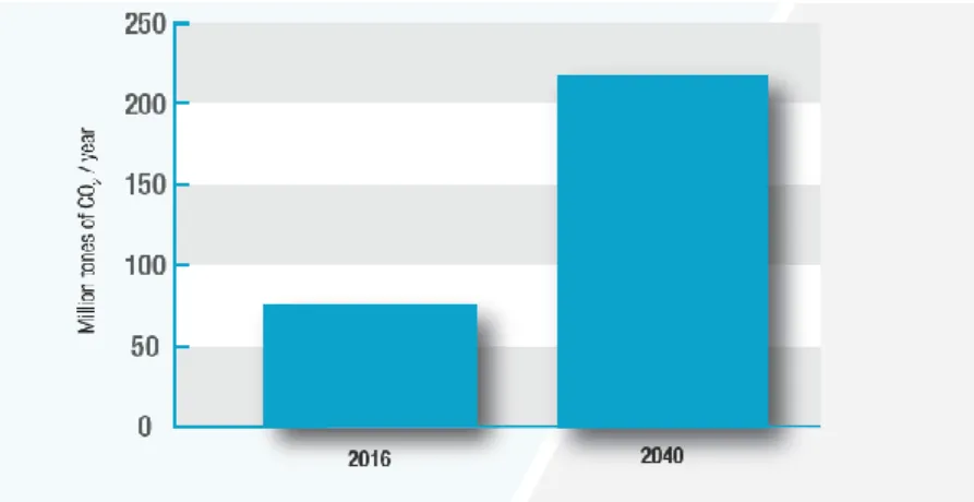
It is expected that in current times, 76 million tons of CO2 is immitted annually due to desalination processes (see Figure 1.5). This number is estimated to rise up to 218 million tons of CO2 per year by 2040 [17]. With an obvious growth on the number of desalination facilities, solar powered desalination can help minimize the ecological footprint left by them. Therefore, the world concerns regarding fossil fuels dependence and greenhouse-gas emissions lead to shifting towards renewable energy sources and desalination is no exception.

(26)

6

Seawater desalination installations and market are growing fast (see Figure 1.6). The Global Water Intelligence (GWI) reports that in 2012 [5], the installed global desalination capacity was increasing by 55% a year.

In 2013 the global installed capacity of desalination freshwater was already 80 million m3_{of fresh water a day [9] and in 2017 nearly 93 million m}3_{a day by around} 18500 desalination plants [10]. The desalination capacity for the next few years is expected to grow 7 to 9% per year worldwide having Asia, the US and Latin America as the main drivers of this growth [9]. The water desalination market is following the same path. It was valued at 13 billion Euros in 2017 and it is expected to grow 7.8% until 2025 [18].

Figure 1.6 - Global Water Desalination Market Size, 2014-2025 (USB Billion) [18].

(27)

7

1.2 - Future Prospects and Objectives in Solar Desalination

There are incredible prospects in developing desalination and RE technologies with an ambitious vision for the future [19]. The long-term use of desalination plants as well as new desalination technologies have resulted in affordable water supply and better energy efficiency [20].

RE desalination costs are still higher than the fossil fuel-powered desalination plants but new studies suggest that the prices are decreasing due to the better process design and better understanding of the technology [21]. The solar energy has the potential to become highly competitive price-wise as it did with other technologies. The use of solar energy for desalination has incredible odds to succeed as a technically practical solution to deal with the water and energy stressing issues.

ProDes took the first step to create an organization to promote renewable energy for water production through desalination with an overall budget of 1,023,594€ in which EU contributed with 75%. Up-to-date there were not any coordination of research nor industrial product development on the European level. It was a project that brought together 14 European organizations to boost the use of RE Desalination with training, workshops, publications and new projects. The creation of “RE Desalination Road Map” defined targets and strategies to enhance the use of RE Desalination technologies where technological, economic and social barriers were tackled.

There is still a strong interest for RE-desalination and taking the ProDes project as an inspiration, other RE-desalination objective-based projects are getting set into practice. Saudi Vision 2030 is a massive project to reduce Saudi Arabia’s dependence on oil, diversify the economy and to modernize the country with the help of foreign investment in every sector.

The energy and water resources are one of the most addressed issues. It was acknowledge the renewable energy potential in the MENA region is huge. MENA region has high annual average wind speed and between 22 and 26% of the world's total direct sun normal irradiation strikes the region [22].

RE-desalination can benefit the region ensuring a sustainable water supply, energy security to the sector and environmental sustainability. The MENA region countries have a pivotal role on the renewable energy desalination, the region is responsible for one third of the world's global desalination capacity.

Jordan, Morocco, Saudi Arabia, The United Arab Emirates and Tunisia have ambitious renewable energy goals in addition to good policies and managerial frameworks to help mature the technology reducing costs and increasing efficiency. In fact, the first big steps are already being made, Al Khafji desalination plant in Saudi

(28)

8

Arabia is the world's first solar-powered desalination plant. With an investment of 114 million euros, it can produce up to 60,000 m3_{of fresh water per day supplying roughly} 150,000 people with safe drinking water [23].

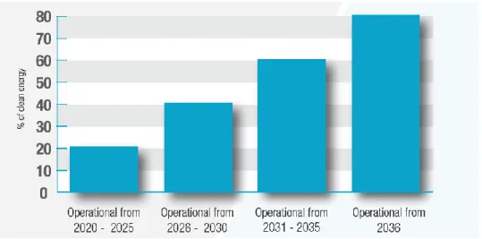
Figure 1.7 – Annual energy to come from clean sources for desalination Plants.

Another challenge is related to the development of small-scale desalination systems, which can be used in a remote location, family residences to small villages, holiday resorts, industrial sites, offshore and marine applications. Research is needed to develop compact, automated and standardized desalination units that can be easily deployable.

As seen in Figure 1.8, small scale desalination installations is still a really small, but with an enormous potential, market ready to be explored.

New studies and roadmaps are being made about the potential of low energy-input, small scale desalination solutions. University of California developed a road-map for small-scale desalination and pointed that choosing the appropriate technology for each specific community is essential for the viability of the project.

The factors are the salinity of available water source, local availability of energy resources such as high wind speeds and total solar irradiance, the capital available, the technical capacity of the population for operation and maintenance and the willingness to take risks with new technologies [24].

Moreover, the study suggested the next steps for the installation of these small-scale desalination solutions being understanding the specific constraints faced by the community involved, using the limitations that will appear can help identify the most suitable technology and pursue help by connecting with relevant technology experts.

(29)

9

Figure 1.8 – Percentage of different desalination plants sizes.

1.3 - SmallSOLDES Project

SmallSOLDES project, aims to develop a reliable and low-maintenance compact solar-driven desalination unit, using an advanced variable geometry ejector and the corresponding control system. The unit consists in two sub-systems interconnected: (1) The solar thermal collectors that will heat the water until temperatures between 120 and 180ºC to be used in the variable geometry ejector, the first part of the (2) Thermal Vapor-Compression (TVC) system. The TVC system will also have a condenser, an evaporator, pre-treatment units, pumps and storage units for the desalination products. The SmallSOLDES project aims to be a water and desalination sustainability reference for the generations to come.

(30)

10

1.4 - Thesis Objectives

This work is being carried within SmallSOLDES project work plan, and the primary objective is to design a Variable Geometry Ejector (VGE) for a solar-driven desalination system. A Computational Fluid Dynamics (CFD) model will be developed to simulate VGE performance with its geometrical details. The model will be based on the compressible Navier-Stokes equation in axi-symmetric coordinates.

The ejector performance will be assessed for a range of relevant operating conditions and distinct geometries. Additionally, VGE performance will be compared to a fixed geometry ejector.

1.5 - Thesis structure

Chapter I introduced an important contextualization about water-stress, energy and sustainability issues. The theoretical background and some important concepts regarding desalination and ejectors will be introduced in Chapter II. Chapter III will introduce the analytical models needed to study the flow inside an ejector with special emphasis on CFD. This chapter will include the introduction and understanding of some turbulence models as well as the mesh refinement process. Chapter IV consists in the simulations details and results using the CFD software FLUENT. This chapter also includes the introduction of simulation, benchmark, analysis of performance characteristics and flow field details of steam ejectors, and optimization of geometric configurations. Chapter V summarizes present work, address the conclusions and suggest possible direction for future work.

(31)

2. Literature Review and

Theoretical Background

Understanding the ejector geometry is key to improve renewable desalination.

2.1 - Desalination

The industrial desalination operation consists in separating nearly salt-free fresh water from the sea or brackish water (see Figure 2.1). The resulting salts are isolated in brine water.

Figure 2.1 - Desalination in a nutshell.

The desalination process can be based on thermal or membrane separation methods. The most important factors affecting the technology choice are the salinity and the temperature of the source water [9].

On the membrane separation processes, Reverse Osmosis (RO) is the most used method. The method consist on moving high pressure brine from one side of membranes to another allowing fresh water to pass through and retain salts, increasing the brine concentration on one side and producing fresh water on the other.

The thermal based separation techniques includes two main categories: (i) Evaporation followed by condensation and (ii) freezing the water followed by melting

(32)

12

the formed water ice crystals. The evaporation followed by condensation method is the most used and it include widely used technologies such as Multistage Flash (MSF), Single effect evaporation and Multi effect evaporation desalination (MED).

Other methods, such as Electrodialysis Reversal Desalination (EDR) uses electricity applied to electrodes to pull naturally occurring dissolved salts through an ion exchange membrane to separate the water from the salts [25].

Table 2.3 summarizes all the advantages and disadvantages of the various commercial desalination methods [22, 26].

2.1.1. – Desalination Energy Consumption

Desalination can, indeed, be the solution for a growing fresh-water scarcity problem. However, the whole process is energy-intensive (see Table 2.1). Desalination consumes more energy per liter than other water supply and treatment options.

Table 2.1 - Energy required to deliver 1m3_{of water for human consumption from}

various water sources [27].

Source Energy Required (kWh/m3₎

Lake or River 0.37

Groundwater 0.48

Wastewater treatment 0.62 – 0.87

Wastewater Reuse 1 – 2.5

Seawater Desalination 2.5 – 8.5

Cost-wise, the energy used in the desalination process represents 5 to 40% of the total operating costs of water and wastewater utilities, depending on the location. This costs will tend to increase, as cities expand further and their water needs increase. Consequently, energy will have direct influence on availability and affordability of water [27].

The energy required for seawater desalination depends on the water temperature and its level of salinity. Most of the energy currently being used to supply most of the energy requirements comes from fossil fuels. However, using fossil fuels represents an unsustainable energy solution that can be replaced by renewable energy sources, specially solar [27].

(33)

13 Due to technological improvements, energy requirements for desalination have declined over the years [28]. Table 2.3 shows the energy values of five desalination techniques that uses renewable energy sources to power the process. It shows that Multi-effect Desalination using a Thermo Vapour Compressor (MED-TVC) is the least energy intensive method of desalination.

2.1.2. – Desalination Economics

Developing trends suggests that thermal desalination and membrane desalination are the most effective methods [21]. In the first few desalination facilities, in the late 1850s, the cost was not important because it was used for military uses producing fresh water for boilers and drinking purposes in ships. When the technology became more widely available for consumers, the costs of fresh water produced became a relevant matter. In 1975 a m3_{of fresh water produced via desalination costed around} 1.85€ [29], now it is estimated to cost, on average, 88 cents per m3_{produced [9].}

To develop a desalination facility, operational costs, the quality of raw water, incentives or subsidies from governments must be considered to have a good financial study of the project. Different desalination methods have different percentages of cost distribution specially when the processes uses different techniques such as membrane separation and thermal separation (see Figure 2.2)

Table 2.2 summarizes the desalination cost of various desalination techniques. It shows that scaling the process can be key to reducing the desalination cost.

Figure 2.2 – Percentage of cost distribution for three desalination methods [30].

(34)

14

The main challenges for renewable energy driven desalination plants are the reduction/financing of initial capital investment for energy generation and the reduction of energy consumption of the desalination process, utilizing more robust energy recovery systems [27].

Table 2.2 - Membrane vs thermal desalination cost per feed water source and production capacity [7].

Current desalination technologies are sensitive to increase in energy prices. Renewable-energy based desalination can eliminate the cost sensibility to energy prices oscillation in the total desalination cost as well as eliminate the carbon emissions of conventional energy supply from the desalination process [28].

Moreover, with the ever decreasing costs of renewable energy production, the association of renewable energy with desalination will permit the implementation of the latter in further locations, leading to the growth of renewable energy desalination markets.

(35)

Table 2.3 - Characteristics of different desalination methods [22, 31-34].

Desalination

Technology MSF MED (Plain) MED-TVC RO EDR

Energy Source Thermal Thermal Thermal Mechanical (via

Electricity) Electricity

Typical energy consumption

(kWh/ m3₎

3-5 1.5-2.5 <1.0 3-5 3-5

Capacity range Up to 90,000 m3_/day _{Up to 38,000 m}3_/day _{Up to 68,000 m}3_/day _{Up to 10,000 m}3_/day _{Up to 34,000 m}3_/day

Typical Salt content

in raw water (ppm) 30,000 – 100,000 30,000 – 100,000 30,000 – 100,000 1000 – 45,000 100-3000

Product water

quality (ppm) <10 <10 <10 <500 <500

Current single train

capacity (m3_/d) 5000 – 60,000 500 – 12,000 100 – 20,000 1 – 10,000 1 – 12,000

Advantages

Easy to manage and operate; Can work with

high salinity water

Suitable to combine with RE sources that supply

intermittent energy

Broad ranges of pressures; Very low electrical

consumption Can operate at low temperatures (<70ºC)

Easy adjustments to local conditions; Best cost in

treating brackish groundwater; Can remove

silica

Recovery rate up to 94% and can be combined with

RO for higher water recovery (up to 98%); Longer-life membranes

(up to 15 years) Disadvantages Do not operate bellow 60%

capacity; High energy use Anti-scalents required Complex configuration

Membrane fouling; Complex configuration

Higher investment associated

(36)

2.1.3. – Thermal Desalination

Distillation is used in thermal desalination, meaning the evaporation and condensation of a fluid. The resulting condensed product is fresh water salt free.

Thermal processes proven to be reliable and having the potential for cogeneration of power and water makes it a very interesting solution capable of replacing MSF technology in future projects [5]. This technology can easily be coupled with the available renewable energy such as ocean energy, solar energy, geo thermal energy etc. and waste heat from power plants [35].

Thermal desalination technologies tend to have low energy intensity [22] and be prone to corrosion. The design of new technological tools should take these issues in consideration, optimizing energy consumption and eliminate sources of corrosion to produce higher quality fresh water [36]. A deep knowledge of thermodynamics and heat mass transfer theory is needed for a complete study and improvement in desalination processes.

Thermodynamics sets the minimum energy required to separate water from a salty solution [6].

2.1.3.1 – Multi-effect Distillation

The multi-effect distillation (MED) is the oldest process in desalination, having references and patents in the literature since 1840. Recent developments in the technology have brought MED to the point of competing technically and economically with MSF, the most widely used thermal desalination process [31]. This new trend is not random, MED systems uses nearly half of the MSF electrical energy and the same amount of thermal energy when both processes have the same gain ratio [37].

In a single effect distillation seawater can be boiled releasing steam that at the time it condenses produces pure water. The MED is based on the same principle but with multiple effects connected making the process more efficient employing falling-film evaporative condensers in a serial arrangement, producing fresh water through repetitive steps of evaporation and condensation.

A normal type of multiple effect distillation is made up of a steam supply unit, a certain number of vessels, a series of preheaters, a train of flashing boxes, a condenser and a venting system. Each vessel (effect) is operated at a lower pressure than the effect

(37)

17 before allowing the seawater feed to sustain multiple boiling effects without exchanging additional heat after the first effect [38].

The seawater begins the distillation process entering the first effect, after being preheated in the tubes, seawater is heated to the boiling point either sprayed or otherwise dispersed onto the surface of the evaporator tubes in a thin layer to boost fast boiling and evaporation. The tubes are heated by steam which is condensed on the opposite side of the tube. The condensate from the boiler steam is recycled to the boiler for reuse [34]. Just part of the seawater put into the tubes is evaporated. The remaining water is reused in the next effect where it is again either sprayed or otherwise dispersed onto the surface of the evaporator tubes.

All the tubes are heated by the vapors created in the previous effect. The vapor is condensed to fresh water, while giving up the heat to evaporate a percentage of the remaining seawater feed in the next effect. Additional condensation happens in each effect which guide the feed water from its source to the first effect. This process increases the water temperature before it is evaporated in the first effect [38]. Figure 2.3 breaks down the entire process.

Figure 2.3 - Diagram of a multi-effect distillation plant.

The number of effects is confined by the temperature difference between the seawater inlet temperature at the first effect and the steam temperature at the last condenser [31] and the minimum temperature differential allowed on each effect [37].

There is a very low drop of temperature per effect (1.5 – 2.5 ºC), enabling the incorporation of a large number of effects resulting in a very high gain ration (product to steam flow ratio) lowering the long-term costs of the desalination process.

The performance of MED can be improved by adding thermal or mechanical vapor compression devices [32]. With the reuse of compressed vapor as heating steam, a significantly reduction on the required steam and boiler sized is obtained.

Additionally, a lower amount of energy is used to operate the system, decreasing even further the operational costs.

(38)

18

2.1.3.2 - Thermal Vapor Compression

Vapor-compressed distillation is mainly used for small and medium-scale water desalination units. The technology is known to be compact and efficient [39] and because of its simplicity and absence of moving parts difficulties and malfunctions are unusual even under extreme conditions.

The new component introduced to the MED system is the steam jet ejector, which acts as a thermal compressor. The steam ejector is used to enhance the efficiency of the system. High temperature and high-pressure motive steam coming from external sources such as a boiler or other power plant is introduced into the ejector.

TVC is responsible for the energy recovery in the MED unit, through transferring the energy contained in the high pressure steam to lower pressure vapor, in order to produce a mixed discharge vapor at intermediate pressure [40].

The compressed vapor is entrained into the first effect as the heat source where it condenses and releases its latent heat inside the tubes. Motive steam compresses part of the cycle last effect vapors after coming from the condenser, while the other part returns to its source [41].

Figure 2.4 - Illustration of MED-TVC system with n effects.

MED-TVC systems have low temperature operation (45-75ºC) [42], hence a better thermal efficiency is obtained making the process one of the most economical seawater desalination processes. It has the ability to use low-cost and low-grade heat.

(39)

19 The new trend in technology development in MED-TVC is using low compression ratios which can reduce the amount of motive steam. This design is compact and provides an approach to increase the unit capacity [41].

Doing a Second Law analysis, the energy quality is determined by its capacity of producing useful work, also known as exergy. Hamed et al. [43] did a study evaluating the performance of TVC and comparing its exergy losses during the process with particular focus on the performance of thermo-compressor. The performance of a TVC system based on exergy analysis was compared in the research against conventional MED systems. Results showed that TVC systems have much better efficiency and lower exergy losses mainly because it reduces the energy consumption required to heat water.

Although TVC systems yield the least exergy destruction among the thermal desalination systems, the most exergy destruction in TVC occurs in the first effect and in the thermo compressor.

Most recently, Alasfour et al. [44] confirmed this fact with exergy analysis simulation models while trying to improve system efficiency. Designing the ejector in optimum conditions is of utmost importance to increase the performance of the whole desalination unit.

(40)

20

2.2 - Ejector

One of the components of a MED-TVC system is the steam ejector, which represents a vital part for the system efficiency. Unlike other compression devices, an ejector can handle two-phase flow, and it is more simple and reliable. An ejector can be used both as a pumping device for incompressible fluids and as a compressor, for compressible fluids. When used as a compressor, a thermal heat source is needed.

An ejector is a mechanism in which a high-velocity jet mixes with a second fluid stream (the entrained flow). The mixture is then discharged with higher pressure than the source of the second fluid. The system operate on the ejector-venturi principle, relying on the momentum of a high-speed steam jet.

A steam ejector is a static device which uses the momentum of a high-speed vapor jet to entrain and accelerate another flow. The thermal compressor is a steam ejector which utilizes the thermal energy to increase the performance by reducing the size of a conventional multi-stage evaporator [45]. The motive fluid can draw large quantities of the secondary fluid because of the lower-pressure at the nozzle exit and high momentum transfer [46]. The nozzle is expected to have a high pressure ratio due to the fact that the poor efficiency of the ejector when operating at low steam pressures [47]. Due to the area reduction and low backpressure, i.e. pressure at the diffuser exit, flow chocking happens at the minimum cross-sectional area where the Mach number is unity [48].

There are different types of ejector designs, being all structurally simple an easy to manufacture, a typical steam-jet air ejector is shown in Figure 2.5. The ejector consists in four parts: (i) primary nozzle, (ii) entrance section, (iii) mixing section and (iv) diffuser.

(41)

21 There are two types of ejector based on how it’s mixing is done. In a Constant Area Mixing (CAM) ejector, the primary nozzle discharge is located in the constant area section and in a Constant Pressure Mixing (CPM) ejector, the nozzle exit is placed downstream in the suction chamber.

Thus, the location of the mixture of the motive and secondary streams is different in CAM ejectors and CPM ejectors. In CPM model it is assumed that the mixing of the primary and the secondary streams occurs in a chamber with a uniform, constant pressure while in the CAM model the mixture occurs in the constant area section. The setup of both the CMA and CPM ejector are shown in Figure 2.6.

The constant-pressure mixing design is the most used design of ejectors because it can provide a more stable and it has the ability to perform at a wider range of backpressures [49].

Figure 2.6 - Two typical ejector types: (a) Constant Pressure Mixing ejector and (b) Constant Area Mixing ejector.

(42)

22

2.2.1 – Operational Conditions

Figure 2.7 demonstrates how the velocity and the pressure change when subsonic (Ma<1) or supersonic (Ma>1) flows face a convergent or a divergent area. This concepts are crucial to understand how the flow works in an ejector.

In the ejector, motive fluid enters a converging diverging nozzle and is accelerated to supersonic conditions. As the flow leaves the nozzle exit section, the supersonic flow creates a low pressure region in the suction chamber which draws the secondary flow to accelerate into the mixing chamber because of the strong shear layer force and increasing the static pressure of the secondary flow (see Figure 2.8 - A). The shear mixing of the two streams begins as the secondary fluid reaches sonic conditions [50]. The stream velocity increases until reaching a supersonic state, where the two fluids are mixed, at the effective area section, then, sudden rise in pressure occurs and flow becomes subsonic again (see Figure 2.8 - B).

The location where the flows are completely mixed, although depending on various operating conditions, should be in the constant area section or in the beginning of the diffuser [51].

As the secondary flow is entrained in the steam, a shockwave is created which leads to subsonic conditions downstream. The mixture then travels through the ejector into a venturi-shaped diffuser. When the steam reaches the diffuser, its kinetic energy is

Figure 2.7 – Velocity and Pressure changes when the flow faces a convergent or divergent area in supersonic and subsonic flows.

(43)

23 converted in pressure energy, which helps to discharge the mixture against a backpressure to the evaporator. About 25 to 50% of the total pressure rise occurs in the diffuser [47].

The motive and the secondary fluids flow towards the lowest-pressure spot. There, both fluids mix together violently and quickly [52]. The mixture, later, slows down and the pressure increase before the mixture comes up at the discharge. Figure 2.8 shows how velocity and pressure vary for the motive and suction fluids through the ejector.

An ejector that can reach supersonic states can work in three different modes regarding the chocking phenomena [51, 53, 54]. In critical mode, double-chocking occurs and the Entrainment Ratio (ER) is constant. The motive and secondary fluids are chocked simultaneously at the constant-area ejector throat under supersonic conditions. The chocking phenomena limits the maximum flow rate of the secondary fluid.

The shock wave is a phenomenon where the flow decreases its Mach speed from supersonic to subsonic conditions.

The shear layer, where is located the shock wave, is at first created by stable vortex-pairing movements helping the mixture of the two fluids. As the flow becomes developed, the large-scale vortexes become reduced in scale, the energy dissipates until a fully developed turbulent flow is reached [55]. With subsonic flow on one side of the shear mixing layer and supersonic flow on the other, the shear layer is stable and steady [48].

(44)

24

Critical back-pressure (see BP* in Figure 2.9.a) is a threshold value corresponding to the critical point and marking the transition between on-design (before the critical point) and off-design (beyond the critical point) conditions [56]. For back-pressure values below the critical back-back-pressure, the entrainment ratio remains constant. This limits as well the maximum Coefficient of performance (COP) value [46]. Once the critical back-Pressure is exceeded, the oblique shock wave moves backward towards the primary nozzle, decreasing the axial velocity of the mixed flow [40, 50].

Increasing the backpressure, subcritical mode is reached (see Sub-Critical mode in Figure 2.9.a) and single-chocking occurs. Only the primary flow is chocked, at the nozzle exit, and there is a linear entrainment ratio relation with the backpressure. A series of oblique and normal shock waves occur and moves the shock wave until reaching the primary nozzle interacting with shear layers. The shock waves have dissipative effects and produces a shift from supersonic to subsonic conditions causing major drops on the performance of the ejector. This will force the primary flow to move back to entrance of the entrained flow.

In the malfunction mode (see Back-Flow in Figure 2.9.a), backflow starts to appearing through the secondary inlet. The phenomena happens when back-pressure is too high to allow entrainment, resulting in over-expanded flow through the nozzle and the development of compression shocks as the motive fluid partially flows back through the entrained fluid inlet [57].

The primary pressure should be as low as possible in order to increase the ejector efficiency and reduce energy costs but high enough to allow the secondary flow to reach sonic speed. When increased, the primary pressure moves the oblique shock wave closer

a. b.

(45)

25 to the diffuser section, increasing the shock intensity, not having significant effect on the entrainment ratio but higher energy spent will be expected. On the other hand, decreasing it below optimum value moves the shock waves closer to the nozzle exit until, similarly to the raise of back-pressure, it causes a reversal flow (see Back-Flow in Figure 2.9.b) [40, 50].

In sum, increasing motive steam pressure above the optimum point will lead to a bigger jet core, smaller effective area, thus lower entrainment ratio. Below the optimum point, the effective area will be bigger than the critical area needed for chocking the secondary flow. In critical conditions, the effective area also reaches critical area in which the secondary flow will start to choke.

The entrainment ratio of an ejector is maximized when the primary flow is perfectly expanded at the nozzle exit and the entrained fluid reaches a chocked condition [58]. In a perfectly expanded flow the compression shocks downstream of the motive fluid come to a halt as the effective flow area of the entrained fluid grows until the static pressure of the motive and the entrained fluid are the same [59]. In normal conditions, perfectly expanded flow is difficult to obtain.

There is normally a certain value of expansion angle. The expansion angle and the supersonic level reached are dependent on the pressure differential between the pressure at the nozzle exit and in the mixing chamber. Over-expanded or under-expanded jets in the mixing section decreases the efficiency of the supersonic ejector [54].

As shown in Table 2.4, in the case of an under-expanded flow, the primary stream will leave the primary nozzle with divergence of expansion angle. Under-expansion happens when the nozzle’s exit pressure is higher than the mixing chamber pressure [61] leading the flow to reach a higher supersonic levels. The increased expansion angle causes the enlargement of the jet core, reducing the effective-area and letting less secondary fluid to be entrained [62].

(46)

26

On the other hand, on an over-expanded flow, the primary stream will leave the primary nozzle with a convergent angle (see Table 2.4). The static pressure at the primary nozzle is lower than the pressure in the mixing chamber, thus the oblique shocks are not as strong as the ones that are produced in an under-expanded flow. Therefore, the flow is more uniform and have less losses in the jet stream’s momentum compared to an under-expanded flow [56, 60, 63].

The mixing process inside the ejector has highly irreversible oblique and normal shocks combined which produces shock diamond-shaped jet. The region where the series of shock waves occurs is called the shock train region.

Diamond-shaped shock-waves indicates partial-separation of high-speed primary flow with the surrounding secondary fluid and produces high shear flow region between both flows [61]. Its location is affected by the converging angle [50, 54, 62].

The converging angle can strongly alter the size of the nozzle and the effective area. Studies suggest that the converging angle should be between 0.5º and 10º [50, 64-67] depending on the ejector type, working fluid and operating conditions. Increasing too much the converging angle leads to higher distances between the ejector walls and the jet core, which can generate excessive pressure gradients that causes boundary layer separation near the wall and backflow [53, 54, 66]. The separation region of the boundary layer gradually increases with the vortexes.

Moreover, the active jet core blocks the way of the secondary flow, preventing it from entrained smoothly into the jet core, decreasing the ejector performance.

On the other hand, decreasing the converging angle too much, making the walls to straightened, leads to a deceleration of the entrained fluid due to a reduction of the flow between the jet core and the wall (virtual nozzle) [54, 62, 68]. As there is less secondary fluid flow, the entrained ratio will decrease.

(47)

27 Considering an idealized case (see Figure 2.10), the effective area is the annulus area between the wall of the ejector mixing area and the primary fluid jet-core [62]. The primary pressure is heavily related to the size of the jet core and effective area. As the primary stream pressure increases, so does the size of the jet core, whilst the effective area decreases.

For a constant secondary pressure and fixed geometry, increasing the temperature and pressure of the motive steam will increase the critical pressure which the ejector can be operated on [50, 63].

However, the ejector entrainment ratio decreases with the increasing of the heat source temperature as shown in Figure 2.11. When the pressure is increased, a smaller effective area is available. Therefore, less amount of the secondary flow is drawn to the mixing chamber while also increasing the primary flow rate [63].

Nonetheless, when having a bigger ejector, increasing the temperature of the primary flow will increase the energy content of the flow, which will reduce the primary flow rate required for the same back-pressure, thus increasing the entrainment ratio [69].

Figure 2.11 - The variation of the entrainment ratio with the primary fluid pressure obtained from CFD simulation [63].

(48)

28

2.2.2 – Ejector design parameters

Obtaining ejectors optimal design is not simple, mainly due to its complex nature of fluid flow mechanisms and its high dependence on working conditions. Entrainment ratio is the most important performance indicator for characterizing the ejector. It is defined as the ratio between the secondary fluid mass flow rate and the primary fluid mass flow. A more detailed explanation and understanding is given bellow in Chapter 3. The most important geometric parameters of an ejector are the Nozzle Exit Position (NXP), suction chamber angle, area ratio (ratio between the constant area section area and the primary nozzle throat), mixing chamber length and the diffuser angle [70]. Out of these parameters, previous studies showed that NXP and the area ratio play a crucial role on the entrainment ratio [68].

2.2.2.1 – Nozzle Exit Position

The NXP can change the performance of the ejector because it affects directly both the entrainment ratio and effective area section. The influence of the optimum NXP increases with increase in active fluid pressure and was found that the performance of the ejector tend to increase with the decrease in NXP (moving the primary nozzle away from the mixing chamber), after which there is a downfall [53, 54, 68]. Thus, there is an optimum value.

The nozzle shape also affects greatly the ejector operation. The ejector works in sub-sonic regime and it can reach, at most, sonic conditions at the suction exit if the nozzle shape is convergent and it works at supersonic velocities if the nozzle is convergent-divergent shaped [46]. The nozzle diverging section is typically conical and its angle should range from 8 to 15 deg [47].

(49)

29

2.2.2.2 – Area Ratio

Defining the optimal value of Area Ratio (AR) is a trade-off process. In fact, the increase in the AR leads to an increase of the entrainment ratio until an optimum value, after that the entrainment ratio starts to drop. A small constant area section diameter leads to a reduction of the effective area for the secondary flow [71]. Increasing the area ratio moves the shock waves upstream, away from the constant area section. It is due to the existence of vortexes in the mixing chamber. Vortexes leads to significant energy losses and reduces mixing efficiency. By increasing the ejector throat diameter, the vortex phenomena is eliminated [53].

The increase in constant area section will increase the entrainment ratio by enhancing suction from the secondary fluid stream but will affect the compression ratio, lowering it and leading to a decrease in critical backpressure [72].

Critical backpressure decreases with the growing of the AR, thus the ejector starts to operate in subcritical mode, single chocking, with lower backpressures (see Figure 2.12).

Figure 2.12 - Effect of the area ratio on the entrainment ratio and critical back-pressure.

As seen in Figure 2.12, diffusers with higher area ratio coefficient tend to have bigger ER values (BP1). However, in situations which is required an higher backpressure, a bigger area ratio can cause malfunction in the ejector (BP2).

(50)

30

2.2.2.3 – Constant Area Section Length

The length of the constant area section also has an influence on controlling the shock wave intensity inside the mixing chamber and the constant area section. To maximize the exit pressure, the mixing chamber has to have a length big enough to let the flow reach subsonic speed.

Thus, critical backpressure increases as the ratio between mixing section length and its diameter increases [73], which allows the ejector to operate in double chocking mode in a wider range of conditions [51].

Moreover, there is an almost linear growth in the entrainment ratio with the extension of the length until an optimum point [74], then it starts to decrease due to total pressure losses that happens at the walls because of shear stress [61] (see Figure 2.13). The outcome of incomplete mixing is inadequate pressure recovery and compression within the diffuser.

Figure 2.13 - Typical behaviour of entrainment ratio with the growth of the length of the mixing chamber.

(51)

31

2.2.2.4 – Diffuser Angle

The diffusers often play an essential role in many applications, therefore many researchers were concerned in diffuser design. The diffuser has a high divergence angle and therefore low efficiency.

The ejector should have an angle range of 5 to 12 deg, or its axial length should go from 4 to 12 times the throat diameter [47]. However this range is not suitable for all the fluids and operating conditions as well [64].

The performance of the diffuser depends largely upon the completeness of mixing in the constant area section [58]. Moreover, the flow reaching the diffuser should be subsonic for a complete use of the diffuser capacities [75]. Otherwise, the flow exiting the diffuser can have a lower pressure and higher velocity than when the flow entered the diffuser.

Moreover, flow separation can occur at the diffuser which can affect the ejector performance, increasing the entropy in the system.

2.2.3 – Variable Geometry Ejector

One of the main characteristic of ejectors is their high level of optimization for certain type of operating conditions. A fixed-geometry ejector can only be optimized for stable fluid properties and is uncapable of providing stable performance with an unstable heat-input [60], which is the case when the heat source comes from a renewable one, where temperature oscillations and intermittency of the source are expected.

To keep entrainment ratio as high as possible on different conditions, variable-geometry technology should be applied [76]. A variable variable-geometry ejector enables performance regulation by adjusting its configuration. Critical backpressure acts as a limit in performance consistency. As the input temperature drops, the critical backpressure falls below the actual pressure, restraining the entrainment ratio by the backpressure and leads to deficient mixing between the two flows, ultimately leading to lower entrainment ratio [77].

On the other hand, with high temperatures, the driving flow rates increases and extra flow cannot be entrained due to the geometrical restriction in the diameter of the mixing chamber [60]. As the motive flows increase and the secondary one remains the same, the energy consumption will be enhanced and the entrainment ratio decreases.