Fertility in Portugal, How persistent is it?

(1)

UNIVERSIDADE DE ÉVORA

DEPARTAMENTO DE ECONOMIA

DOCUMENTO DE TRABALHO Nº 2005/12

July

Fertility in Portugal

How persistent is it?

1

st

_{version: January 31, 2005}

This version: July 12, 2005

Maria Filomena Mendes

2

Universidade de Évora, Departamento de Sociologia

Gertrudes Guerreiro

Universidade de Évora, Departamento de Economia

António Caleiro

Universidade de Évora, Departamento de Economia

1

We would like to acknowledge the financial support from Fundação da Ciência e Tecnologia (Project

POCTI/DEM/59445/2004)

2

Corresponding author. Address: Universidade de Évora, Departamento de Sociologia, Largo dos

Colegiais, 2, 7002-883 Évora, Portugal, Tel. + 351266 740 805, Fax: + 351 266 740 809

UNIVERSIDADE DE ÉVORA

DEPARTAMENTO DE ECONOMIA

Largo dos Colegiais, 2 – 7000-803 Évora – Portugal

Tel.: +351 266 740 894 Fax: +351 266 742 494

(2)

Abstract

:

The decline in fertility that has been observed in Portugal is an apparent fact. From 1960 to 2002, the

average number of children by woman has decreased from 3.1 to 1.5.

Not ignoring this strong evidence of a sustainable decrease in fertility, the fact is that the numbers on the

fertility rates by women’ ages show different realities. At the first sight, the decline in fertility of younger

women has been the result of a postponement of births given that a general increase in fertility rates has

been observed for older women. A question that then comes up is the following: are these observed

trajectories sustainable in the sense of reflecting persistence in time or are just mere phases of a cycle in

fertility? The paper intents to start giving an answer to that question by the use of statistical techniques, in a

univariate approach, which are adequate to measure the degree of persistence over time.

Keywords:

Fertility, Persistence, Portugal

JEL Classification:

C22, J11, J13

(3)

1. Introduction and motivation

This paper considers the fertility rates for Portuguese women aged between 16 and 48

years old for the period 1971-2002.

3

_{Figure 1 gives a picture of the evolution registered}

by fertility.

Figure 1 – The evolution of fertility in Portugal [1971-2002]

Clearly, in the overall, there seems to exist evidence of a sustainable decrease in fertility

but it is also true that the numbers on the fertility rates by women ages show different

realities. At the first sight, the decline in fertility of younger women has been the result

of a postponement of births given that a general increase in fertility rates has been

observed for older women. A question that then comes up is the following: are these

observed trajectories sustainable in the sense of reflecting persistence in time or are

just mere phases of a cycle in fertility? The paper intents to start giving an answer to

that question by the use of statistical techniques, in a univariate approach, which are

adequate to measure the degree of persistence over time. Before doing that, an aspect of

apparent importance, as it is the correlation between fertility rates, is to be presented.

In fact, in accordance to figure 1, it seems that, despite the inevitable high correlation,

in fertility, for women with close ages, given the usual time lag between births, the

correlation may increase after a certain amount of time. This is certainly important to

3

(4)

be taken into account in the assessment of the results in what concerns the detection of

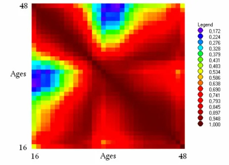
the women’s ages for which fertility is more persistent. Figure 2 plots the correlation

coefficient of fertility among the distinct ages.

Figure 2 – The correlation between fertility rates

Generally speaking, what figure 2 shows is that the correlation coefficient of fertility

rates decreases when the distance in ages increases but only to a certain distance, as for

certain ages, women sufficiently separated in age are more similar, in terms of fertility.

That being said, the rest of the paper has the following structure. Section 2 analyses the

fertility persistence. Section 3 concludes.

2. Measuring fertility persistence in Portugal

As the previous section has shown, in accordance to the women’s ages, the fertility rates

in Portugal have gone through evolutions that are clearly distinct. A question that then

comes up is the following: are these observed trajectories sustainable in the sense of

reflecting persistence in time or are just mere phases of a cycle in fertility? We start

giving an answer to this question by the use of statistical techniques, in a univariate

approach, which are adequate to measure the degree of persistence over time.

(5)

Since some time ago, some authors have started to pay attention to persistence in

(economic) time series as a phenomenon that reveals to be crucial to policy measures,

namely at the inflation level. In fact, to the best of our knowledge, all the applications of

the statistical techniques to measure the level of persistence have considered the

inflation rate case. See Hondroyiannis and Lazaretou (2004), Levin and Piger (2002),

Marques (2004), Minford et al. (2004), and Pivetta and Reis (2004). We propose to

apply those statistical techniques, developed by Andrews and Chen (1994), Dias and

Marques (2004) and Marques (2004), to fertility rates in Portugal. In this sense, the

novelty in the approach is supposed to be a contribution to filling the gap in the

demographics literature.

Starting with a simple definition, fertility persistence is the speed with which fertility

returns to baseline (its previous level) after, say a shock, i.e. some event (for instance, a

demographic policy measure) that provoked an increase (or decrease) in the fertility

rate. This definition, in other words, implies that the degree of fertility persistence is

associated with the speed with which fertility responds to a shock. When the value is

high, fertility responds quickly to a shock. On the contrary, when the value is small, the

speed of adjustment by fertility is low. To put it clearer, a variable is said to be the more

persistent the slower it converges or returns to its previous level, after the occurrence of

a shock.

Quantifying the response of fertility to a shock is indeed important not only because it

may allow assessing the effectiveness of demographic policy measures but also because

it may, indeed, show at what time is more essential to act, through those measures, in

order to overwhelm a harmful effect of a shock over fertility. By definition, quantifying

the response of fertility to shocks implies evaluating the persistence of fertility.

As the estimates of persistence at time t will express how long we expect that a shock to

fertility will take to die off (if ever), given present and past fertility, authors have

proposed to obtain those estimates by the use of autoregressive models. As it is well

known, a univariate AR(k) process is characterised by the following expression:

(1)

∑

= −

+

=

k j t j t j t

f

1

ε

α

µ

(6)

where

f

_t

denotes the fertility rate at moment t, which is explained by a constant

µ

, by

past values up to lag k, as well as by a number of other factors, whose effect is captured

by the random variable

ε

t

. Plainly, (1) can also be written as:

(2)

∑

(

)

− = − −

+

−

+

∆

+

=

∆

1 1 1

1

k j t t j t j t

f

µ

δ

ρ

ε

where

(3)

1 k j j

ρ

α

=

∑

and

∑

+ =

−

=

k j i i j 1

α

δ

.

In the context of the above model (1), or (2), persistence can be defined as the speed

with which fertility converges to its previous level after a shock in the disturbance term

that raises fertility at moment t by 1%.

4

The techniques allowing for measuring the persistence are based on the analysis of the

autoregressive coefficients

α

_j

in (1) or (2), which are subject to a statistical estimation.

Plainly, the most simple case of the models (1) or (2) is the so-called AR(1) model, that

is:

(4)

f

_j

= +

µ α

₁

f

_t₋₁

+

ε

_t

.

Clearly, the variable

ε

_t

in this kind of models has a particular importance given that it

may be associated with policy measures leading to a shock in the fertility rates. A

positive shock, at moment t, will significantly last for future moments the higher is the

4

Given that the persistence is a long-run effect of a shock to fertility, this concept is intimately

linked to a concept usually associated to autoregressive models such as (1) or (2), i.e. the

impulse response function of fertility, which, in fact, is not a useful measure of persistence since

its infinite length.

(7)

autoregressive coefficient

α

₁

. Following this approach, Andrews and Chen (1994)

proposed the sum of the autoregressive coefficients,

∑

=

k j j 1

α

ρ

, as a measure of

persistence.

5

_{The rationale for this measure comes from realizing that for}

ρ

<

₁

_{, the}

cumulative effect of a shock on fertility is given by

1

1 −

ρ

.

Following the approach above described, some autoregressive models (1) were

estimated for Portugal, considering all women’s ages between 16 and 48, for the period

1971 to 2002. The results can be consulted in the Appendix 1.

A general comment on the obtained results is that, not surprisingly, for many ages, a

simple AR(1) (with or without constant) appears to be a congruent model in explaining

the fertility rate. Yet there are a non ignorable number of cases where a higher order

autoregressive model is suggested by the data. This fact poses a problem from the

viewpoint of measuring persistence in the fertility rates, as it will be described below.

Quite recently, Marques (2004) has suggested a non-parametric measure of

persistence, γ, based on the relationship between persistence and mean reversion. In

particular, Marques (2004) suggested using the statistic:

(5)

T

n

−

=

1 γ

,

where n stands for the number of times the series crosses the mean during a time

interval with T + 1 observations, to measure the absence of mean reversion of a given

series, given that it may be seen as the unconditional probability of that given series not

crossing its mean in period t.

6

5

Authors have, indeed, proposed other alternative measures of persistence, such as the largest

autoregressive root, the spectrum at zero frequency, or the so called half-life. For a technical

appraisal of these other measures see, for instance, Marques (2004) and Dias and Marques

(2004).

6

_{As acknowledged in Marques (2004), values close to 0.5 indicate the absence of any significant}

persistence (white noise behaviour) while figures significantly above 0.5 signal significant

(positive) persistence.

(8)

As Dias and Marques (2004) have shown, there is a one-to-one correspondence

between the sum of autoregressive coefficients,

ρ

, given by (3) and the non-parametric

measure,

γ

, given by (5), when the data are generated by an AR(1) process, but such a

one-to-one correspondence ceases to exist once higher order autoregressive processes

are considered. In other words, only in the particular case of a first-order

autoregressive model, AR(1), either one of the two measures can be used to quantify the

level of persistence, as both transmit the same result, but as soon as higher order

autoregressive models are considered, i.e., AR(k) with

k

≥

2 , the monotonic

relationship between

ρ

and

γ

no longer exists, therefore leading to possibly crucial

differences when measuring persistence in the series.

As Dias and Marques (2004) plainly show, using the alternative measure of persistence,

γ

, given by (5), has some important advantages.

7

_{Given its nature, such measure of}

persistence does not impose the need to assume a particular specification for the data

generation process, therefore does not require a model for the series under

investigation to be specified and estimated.

8

_{This is so given that}

γ

_{is indeed extracting}

all the information about the persistence from the data itself. As it measures how often

the series reverts to its means and (high/low) persistence exactly means that, after a

shock, the series reverts to or crosses its means more (seldom/frequently), one does not

need to specify a particular form for the data generation process.

That being said, it resulted clear that, in order to measure the persistence in the fertility

rates in Portugal, one should rely on the use of the non-parametric measure

γ

. Clearly,

in order to compute the estimative for each women’s age, the mean of each series has to

be computed. As suggested in Marques (2004), a time varying mean is more

appropriate than the simple average for all the period under investigation. In our case

we followed that suggestion by using the well known Hodrick-Prescott (HP) filter in

order to compute the mean.

As it is well known, the HP filter defines the trend or mean,

g

_t

, of a time series,

f

_t

, as

the solution to the minimisation problem:

7

_{The statistical properties of}

γ

_{are extensively analysed in Marques (2004) and Dias and}

Marques (2004).

8

In technical terms, this means that the measure is expected to be robust against potential

model misspecifications and given its non-parametric nature also against outliers in the data.

(9)

{ }

(

)

(

) (

)

_











−

+

−

∑

= − = + − T t T t t t t t t t gt ₁

f

g

1 2 2 1 1 2

min

λ

i.e. the HP-filter seeks to minimise the cyclical component

(

f

_t

−

g

_t

)

subject to a

smoothness condition reflected in the second term. The higher the parameter

λ

, the

smoother will be the trend and the less deviations from trend will be penalised. In the

limit, as

λ

goes to infinity, the filter will choose

(

g

t+1

−

g

t

) (

=

g

t

−

g

t−1

)

, for

2,...,

1 t

=

T

−

, which just amounts to a linear trend. Conversely, for

λ

=

0 , we get the

original series.

Plainly, the HP-filter is a very flexible device since it allows us to approximate many

commonly used filters by choosing appropriate values of

λ

. Given that the data is of

yearly frequency, authors have suggested using values for

λ

between 7 and 13. In order

to check the robustness of the results we considered all these values when computing

the estimates of

γ

. See the Appendix 2, where the pictures corresponding to the

10 λ

=

case are also shown.

From the results, one can conclude that there are two particular groups of women that

reveal to possess higher levels of fertility persistence. The first group is composed by

women with ages between 22 and 25 years old, notably 24 years old, and a second

group composed by women whose age is 30 or 31 years old.

3. Conclusion and directions for further research

This paper has explored the question of fertility persistence in Portugal. The main

conclusion is that there are two groups of women that are of particular relevance for

demographic policy measures, namely women between 22 and 25 years and those aged

between 30 and 31 years old.

As directions for further research we would like to further explore the lagged

correlation analysis in order to discern about the moment in time where women started

to change their relative behaviour towards fertility.

(10)

References

Andrews, D., and W.K. Chen (1994), “Approximately Median-Unbiased Estimation of

Autoregressive Models”, Journal of Business and Economic Statistics, 12, 187-204.

Dias, Daniel, and Carlos Robalo Marques (2004), “Using Mean Reversion as a Measure

of Persistence”, Working Paper Series N.º 450, European Central Bank, March.

Hondroyiannis, George, and Sophia Lazaretou (2004), “Inflation Persistence during

Periods of Structural Change: An assessment using Greek data”, Working Paper 13,

June.

Levin, Andrew T., and Jeremy M. Piger (2002), “Is Inflation Persistence Intrinsic In

Industrial Economies?”, Working Paper 2002-023E, Federal Reserve Bank of St.

Louis, October.

Marques, Carlos Robalo (2004), “Inflation Persistence: Facts or Artefacts?”, Working

Paper 8, Banco de Portugal, June.

Minford, Patrick, Reic Nowell, Prakriti Sofat, and Naveen Srinivasan (2004), “UK

Inflation Persistence: Policy or Nature”, mimeo, Cardiff University.

Pivetta, Frederic, and Ricardo Reis (2004), “The Persistence of Inflation in the United

States”, mimeo, Harvard University.

(11)

Appendix 1 – The statistical results for the autoregressive models

Modelling FRate16 by OLS (using FRateP.in7) The present sample is: 1972 to 2002

Variable Coefficient Std.Error t-value t-prob PartR^2 FRate16_1 0.99399 0.019432 51.153 0.0000 0.9890

R^2 = 0.989039 \sigma = 0.00141509 DW = 1.63 * R^2 does NOT allow for the mean *

RSS = 5.807175301e-005 for 1 variables and 31 observations

Variable Coefficient Std.Error t-value t-prob PartR^2 FRate17_1 1.3524 0.17607 7.681 0.0000 0.6782 FRate17_2 -0.36100 0.17505 -2.062 0.0486 0.1319

RSS = 0.0001368276735 for 2 variables and 30 observations

(12)

* R^2 does NOT allow for the mean *

Variable Coefficient Std.Error t-value t-prob PartR^2 Constant 0.0093202 0.0046531 2.003 0.0546 0.1215 FRate27_1 0.90334 0.038419 23.513 0.0000 0.9502

R^2 = 0.95016 F(1,29) = 552.86 [0.0000] \sigma = 0.00402936 DW = 2.32 RSS = 0.000470837209 for 2 variables and 31 observations

(13)

Variable Coefficient Std.Error t-value t-prob PartR^2 Constant 0.0072273 0.0024296 2.975 0.0061 0.2468 FRate33_1 1.3109 0.16253 8.066 0.0000 0.7067 FRate33_2 -0.43015 0.14427 -2.982 0.0060 0.2477

(14)

The present sample is: 1973 to 2002

R^2 = 0.983634 F(2,26) = 781.35 [0.0000] \sigma = 0.00145043 DW = 1.77 RSS = 5.469763919e-005 for 3 variables and 29 observations

(15)

(16)

The present sample is: 1972 to 2002

(17)

Appendix 2 –

Mean reversion in the Portuguese fertility rates

Table 1: The values for the

γ

statistic

λ = 7

λ = 8

λ = 9

λ = 10

λ = 11

λ = 12

λ = 13

16 years old

0.419355 0.419355 0.419355 0.419355 0.419355 0.419355 0.419355

17 years old

0.483871 0.483871 0.483871 0.483871 0.483871 0.483871 0.483871

18 years old 0.580645 0.580645 0.580645 0.580645 0.580645 0.580645 0.580645

19 years old 0.580645 0.580645 0.580645 0.580645 0.580645 0.580645 0.580645

20 years old 0.451613 0.451613 0.451613 0.451613 0.451613 0.516129 0.516129

21 years old

0.516129 0.516129 0.516129 0.516129 0.516129 0.516129 0.516129

22 years old

0.645161 0.709677 0.709677 0.645161 0.645161 0.645161 0.645161

23 years old

0.645161 0.645161 0.645161 0.645161 0.645161 0.645161 0.645161

24 years old 0.677419 0.677419 0.677419 0.741935 0.741935 0.741935 0.741935

25 years old 0.580645 0.580645 0.580645 0.645161 0.709677 0.709677 0.709677

26 years old

0.516129 0.516129 0.516129 0.516129 0.516129 0.516129 0.516129

27 years old 0.612903 0.612903 0.612903 0.612903 0.645161 0.645161 0.645161

28 years old 0.548387 0.548387 0.548387 0.548387 0.548387 0.548387 0.548387

29 years old 0.548387 0.548387 0.548387 0.548387 0.548387 0.548387 0.548387

30 years old 0.645161 0.645161 0.645161 0.645161 0.645161 0.645161 0.645161

31 years old

0.645161 0.645161 0.645161 0.645161 0.645161 0.645161 0.645161

32 years old

0.516129 0.516129 0.516129 0.516129 0.516129 0.516129 0.580645

33 years old 0.548387 0.548387 0.612903 0.612903 0.612903 0.612903 0.612903

34 years old 0.419355 0.419355 0.419355 0.483871 0.483871 0.483871 0.483871

35 years old 0.548387 0.612903 0.612903 0.612903 0.612903 0.612903 0.677419

36 years old 0.483871 0.483871 0.483871 0.483871 0.483871 0.483871 0.548387

37 years old 0.612903 0.612903 0.612903 0.612903 0.677419 0.677419 0.677419

38 years old 0.580645 0.580645 0.580645 0.580645 0.580645 0.612903 0.677419

39 years old 0.483871 0.483871 0.483871 0.483871 0.483871 0.483871 0.483871

40 years old 0.516129 0.516129 0.516129 0.516129 0.516129 0.516129 0.516129

41 years old 0.548387 0.548387 0.548387 0.548387 0.612903 0.612903 0.612903

42 years old 0.387097 0.387097 0.387097 0.387097 0.451613 0.483871 0.483871

43 years old 0.483871 0.483871 0.483871 0.483871 0.483871 0.483871 0.483871

44 years old 0.419355 0.419355 0.419355 0.419355 0.419355 0.419355 0.419355

45 years old 0.387097 0.387097 0.387097 0.387097 0.387097 0.387097 0.387097

46 years old 0.419355 0.419355 0.419355 0.419355 0.419355 0.419355 0.419355

47 years old 0.548387 0.548387 0.548387 0.548387 0.548387 0.548387 0.548387

48 years old 0.354839 0.354839 0.354839 0.354839 0.354839 0.354839 0.354839

(18)

The

λ

=

10 case

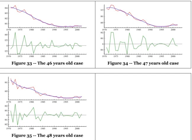
N.B. – In all the figures, the top panel displays the fertility rates (in red) and

the mean of the fertility rates (in blue) whereas the bottom panel displays the

deviations from the mean

1970 1975 1980 1985 1990 1995 2000 .01 .015 .02 1970 1975 1980 1985 1990 1995 2000 -.002 0 .002

Figure 3 -- The 16 years old case

1970 1975 1980 1985 1990 1995 2000 .02 .025 .03 .035 .04 1970 1975 1980 1985 1990 1995 2000 -.0025 0 .0025 .005

1970 1975 1980 1985 1990 1995 2000 .03 .04 .05 .06 .07 1970 1975 1980 1985 1990 1995 2000 0 .005

1970 1975 1980 1985 1990 1995 2000 .04 .06 .08 .1 1970 1975 1980 1985 1990 1995 2000 -.005 0 .005 .01

1970 1975 1980 1985 1990 1995 2000 .05 .075 .1 .125 1970 1975 1980 1985 1990 1995 2000 -.005 0 .005 .01 .015

1970 1975 1980 1985 1990 1995 2000 .05 .1 .15 1970 1975 1980 1985 1990 1995 2000 -.005 0 .005 .01 .015

(19)

1970 1975 1980 1985 1990 1995 2000 .1 .15 1970 1975 1980 1985 1990 1995 2000 -.005 0 .005 .01

1970 1975 1980 1985 1990 1995 2000 .1 .15 1970 1975 1980 1985 1990 1995 2000 -.005 0 .005 .01 .015

1970 1975 1980 1985 1990 1995 2000 .1 .15 1970 1975 1980 1985 1990 1995 2000 -.005 0 .005

1970 1975 1980 1985 1990 1995 2000 .1 .125 .15 .175 1970 1975 1980 1985 1990 1995 2000 -.005 0 .005

1970 1975 1980 1985 1990 1995 2000 .1 .12 .14 .16 1970 1975 1980 1985 1990 1995 2000 -.005 0 .005

1970 1975 1980 1985 1990 1995 2000 .1 .12 .14 1970 1975 1980 1985 1990 1995 2000 -.005 0 .005

1970 1975 1980 1985 1990 1995 2000 .09 .1 .11 .12 .13 1970 1975 1980 1985 1990 1995 2000 -.005 0 .005

(20)

1970 1975 1980 1985 1990 1995 2000 .09 .1 .11 .12 .13 1970 1975 1980 1985 1990 1995 2000 -.005 0 .005

1970 1975 1980 1985 1990 1995 2000 .08 .1 .12 1970 1975 1980 1985 1990 1995 2000 -.005 0

1970 1975 1980 1985 1990 1995 2000 .06 .08 .1 .12 1970 1975 1980 1985 1990 1995 2000 -.0025 0 .0025

1970 1975 1980 1985 1990 1995 2000 .06 .08 .1 1970 1975 1980 1985 1990 1995 2000 -.0025 0 .0025 .005

1970 1975 1980 1985 1990 1995 2000 .06 .08 .1 1970 1975 1980 1985 1990 1995 2000 -.005 0 .005

1970 1975 1980 1985 1990 1995 2000 .04 .06 .08 1970 1975 1980 1985 1990 1995 2000 -.005 0 .005

1970 1975 1980 1985 1990 1995 2000 .04 .06 .08 1970 1975 1980 1985 1990 1995 2000 -.005 -.0025 0 .0025

1970 1975 1980 1985 1990 1995 2000 .03 .04 .05 .06 .07 1970 1975 1980 1985 1990 1995 2000 -.0025 0 .0025

(21)

1970 1975 1980 1985 1990 1995 2000 .02 .03 .04 .05 .06 .07 1970 1975 1980 1985 1990 1995 2000 -.002 0 .002

1970 1975 1980 1985 1990 1995 2000 .02 .03 .04 .05 .06 1970 1975 1980 1985 1990 1995 2000 -.002 -.001 0 .001 .002

1970 1975 1980 1985 1990 1995 2000 .01 .02 .03 .04 .05 1970 1975 1980 1985 1990 1995 2000 -.001 0 .001 .002 .003

1970 1975 1980 1985 1990 1995 2000 .01 .02 .03 .04 1970 1975 1980 1985 1990 1995 2000 -.001 0 .001

1970 1975 1980 1985 1990 1995 2000 .01 .02 .03 1970 1975 1980 1985 1990 1995 2000 -.002 -.001 0 .001 .002

1970 1975 1980 1985 1990 1995 2000 .005 .01 .015 .02 .025 1970 1975 1980 1985 1990 1995 2000 -.0005 0 .0005 .001

1970 1975 1980 1985 1990 1995 2000 .005 .01 .015 1970 1975 1980 1985 1990 1995 2000 -.0005 0 .0005 .001

1970 1975 1980 1985 1990 1995 2000 .0025 .005 .0075 1970 1975 1980 1985 1990 1995 2000 -.0002 0 .0002 .0004

(22)

1970 1975 1980 1985 1990 1995 2000 .001 .002 .003 .004 1970 1975 1980 1985 1990 1995 2000 -.00025 0 .00025 .0005

1970 1975 1980 1985 1990 1995 2000 .0005 .001 .0015 1970 1975 1980 1985 1990 1995 2000 -.0001 0 .0001 .0002

1970 1975 1980 1985 1990 1995 2000 .0005 .001 1970 1975 1980 1985 1990 1995 2000 -.0002 -.0001 0 .0001 .0002